www.ssoar.info

The two Hindenburg elections of 1925 and 1932: atotal reversal of voter coalitions [1990]Falter, Jürgen W.

Veröffentlichungsversion / Published VersionZeitschriftenartikel / journal article

Zur Verfügung gestellt in Kooperation mit / provided in cooperation with:GESIS - Leibniz-Institut für Sozialwissenschaften

Empfohlene Zitierung / Suggested Citation:Falter, Jürgen W.: The two Hindenburg elections of 1925 and 1932: a total reversal of voter coalitions [1990]. In:Historical Social Research, Supplement (2013), 25, pp. 217-232. URN: http://nbn-resolving.de/urn:nbn:de:0168-ssoar-379952

Nutzungsbedingungen:Dieser Text wird unter einer CC BY-NC-ND Lizenz(Namensnennung-Nicht-kommerziell-Keine Bearbeitung) zurVerfügung gestellt. Nähere Auskünfte zu den CC-Lizenzen findenSie hier:http://creativecommons.org/licenses/

Terms of use:This document is made available under a CC BY-NC-ND Licence(Attribution Non Comercial-NoDerivatives). For more Informationsee:http://creativecommons.org/licenses/

Historical Social Research Supplement 25 (2013) 217-232 │© GESIS

The Two Hindenburg Elections of 1925 and 1932: A Total Reversal of Voter Coalitions [1990]

Jürgen W. Falter ∗

Abstract: »Die Hindenburg-Wahlen von 1925 und 1932: Eine vollständige Um-kehrung der Wähler-Koalitionen«. This article compares the two presidential elections of 1925 and 1932 in an attempt to determine the shifts between these two elections which brought Paul von Hindenburg to power. Although this article does not attempt to add to the historiography of Hindenburg’s elec-tion and the subsequent deparliamentarization which has often been thought by historians to have eased Hitler’s transition to power, it attempts to use sta-tistical verification to underline a number of hypotheses generally agreed upon by historians, but which lack substantial evidence. In considering Hindenburg’s election, a number of variables are considered, such as: which parties the Hin-denburg voters came from, why Hindenburg was backed rather than his oppo-sitional candidate Wilhelm Marx, and what social background the Hindenburg voters had. Also, the commonly held belief that many of the communist voters fluctuated from the communist party candidate, Ernst Thälmann, to Adolf Hit-ler is statistically analyzed. Keywords: Hindenburg, deparliamentarization, Weimar Republic.

1. Introductory Remarks

The two Weimar presidential elections of March and April, 1925 and 1932, are among the most fascinating and historically significant elections of modern German history (see Table 1). They are fascinating for the electoral historian and the generalist alike because of the virtually total reversal between 1925 and 1932 of the voting coalitions that backed and brought to power the aged Field Marshal Paul von Hindenburg. And they are historically extremely significant because it was von Hindenburg who at least encouraged if not sustained the creeping process of deparliamentarization after 1930, a process that finally brought Hitler into power. It may be readily speculated that another president, e.g., Wilhelm Marx, who as the candidate of the Weimar coalition parties was Hindenburg’s chief opponent in 1925, would not so easily have dismissed Reich Chancellor Heinrich Brüning in May of 1932. And Marx undoubtedly

∗ Reprint of: Falter, Jürgen W. 1990. The Two Hindenburg Elections of 1925 and 1932: A Total

Reversal of Voter Coalitions. Central European History 23, 225-41.

HSR Suppl. 25 (2013) │ 218

would not have appointed the right-wing Center party dissident, Franz von Papen, as Brüning’s successor.

Astonishingly, these two really important Weimar elections have yet to be adequately investigated by electoral historians. An analysis of these elections therefore virtually has to start from scratch. The outcome does not, perhaps, necessarily add something new to what has been assumed by historians about the two Hindenburg elections. The significance of the following analysis lies more in the fact that it provides statistical confirmation for some more or less commonly held but never sufficiently corroborated hypotheses. In the follow-ing, I will turn first to the 1925 election in order to find out where – i.e., what parties – the Hindenburg voters came from, and what role was played by the decision of the Catholic Bavarian People’s Party (BVP) to back Hindenburg instead of the candidate of the Catholic Center Party, Wilhelm Marx. Then I will examine the transition from 1925 to 1932. I will ask what statistical rela-tions may be observed between these two elections and, from a complementary perspective, what social groups supported Hindenburg in 1925 and 1932, re-spectively. In a third and final step I will try to find out if there really was a significant voter fluctuation between the Communist candidate Ernst Thälmann and Adolf Hitler from the first to the second ballot of 1932, as is so often al-leged in contemporary and historical analyses of the collapse of the Weimar Republic.

2. From what Parties did the 1925 Hindenburg Voters Come, and to what Parties did they go in Subsequent Elections?

Of course this question cannot be answered directly or beyond any reasonable doubt, since we do not have any methodologically reliable and representative opinion polls for the Weimar period. What we can do, however, is to look first at the statistical relationship between the Hindenburg vote and the vote of other parties and candidates at the level of the 1,200 German counties and cities of that period. The results are statistically sound if we restrict the verbal interpre-tation of our findings to the territorial, that is, the county, level. Since we are, however, much more interested in individual-level relationships, I will try, in a second – statistically somewhat risky – step, to discern the underlying (but unknown) “true” voting transitions to and from Hindenburg by means of multi-ple ecological regression analysis.1

1 This analytical tool was first proposed by the German statistician Fritz Bernstein (“Über eine

Methode, die soziologische und bevölkerungsstatistische Gliederung von Abstimmungen bei geheimen Wahlverfahren statistisch zu ermitteln,” Allgemeines Statistisches Archiv 22

HSR Suppl. 25 (2013) │ 219

2.1 Some Party-Vote Correlations of the 1925 Hindenburg Vote

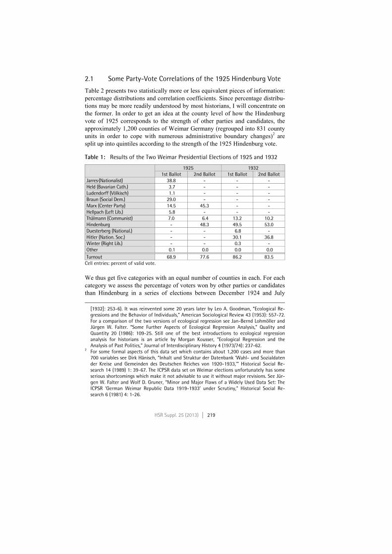
Table 2 presents two statistically more or less equivalent pieces of information: percentage distributions and correlation coefficients. Since percentage distribu-tions may be more readily understood by most historians, I will concentrate on the former. In order to get an idea at the county level of how the Hindenburg vote of 1925 corresponds to the strength of other parties and candidates, the approximately 1,200 counties of Weimar Germany (regrouped into 831 county units in order to cope with numerous administrative boundary changes)2 are split up into quintiles according to the strength of the 1925 Hindenburg vote.

Table 1: Results of the Two Weimar Presidential Elections of 1925 and 1932

1925 1932

1st Ballot 2nd Ballot 1st Ballot 2nd Ballot Jarres·(Nationalist) 38.8 - - - Held (Bavarian Cath.) 3.7 - - - Ludendorff (Völkisch) 1.1 - - - Braun (Social Dem.) 29.0 - - - Marx (Center Party) 14.5 45.3 - - Hellpach (Left Lib.) 5.8 - - - Thälmann (Communist) 7.0 6.4 13.2 10.2 Hindenburg - 48.3 49.5 53.0 Duesterberg (National.) - - 6.8 - Hitler (Nation. Soc.) - - 30.1 36.8 Winter (Right Lib.) - - 0.3 - Other 0.1 0.0 0.0 0.0 Turnout 68.9 77.6 86.2 83.5

Cell entries: percent of valid vote. We thus get five categories with an equal number of counties in each. For each category we assess the percentage of voters won by other parties or candidates than Hindenburg in a series of elections between December 1924 and July

[1932]: 253-6). It was reinvented some 20 years later by Leo A. Goodman, “Ecological Re-gressions and the Behavior of Individuals,” American Sociological Review 43 (1953): 557-72. For a comparison of the two versions of ecological regression see Jan-Bernd Lohmöller and Jürgen W. Falter. “Some Further Aspects of Ecological Regression Analysis,” Quality and Quantity 20 (1986): 109-25. Still one of the best introductions to ecological regression analysis for historians is an article by Morgan Kousser, “Ecological Regression and the Analysis of Past Politics,” Journal of Interdisciplinary History 4 (1973/74): 237-62.

2 For some formal aspects of this data set which contains about 1,200 cases and more than 700 variables see Dirk Hänisch, “Inhalt und Struktur der Datenbank ‘Wahl- und Sozialdaten der Kreise und Gemeinden des Deutschen Reiches von 1920-1933,’” Historical Social Re-search 14 (1989) 1: 39-67. The ICPSR data set on Weimar elections unfortunately has some serious shortcomings which make it not advisable to use it without major revisions. See Jür-gen W. Falter and Wolf D. Gruner, “Minor and Major Flaws of a Widely Used Data Set: The ICPSR ‘German Weimar Republic Data 1919-1933’ under Scrutiny,” Historical Social Re-search 6 (1981) 4: 1-26.

HSR Suppl. 25 (2013) │ 220

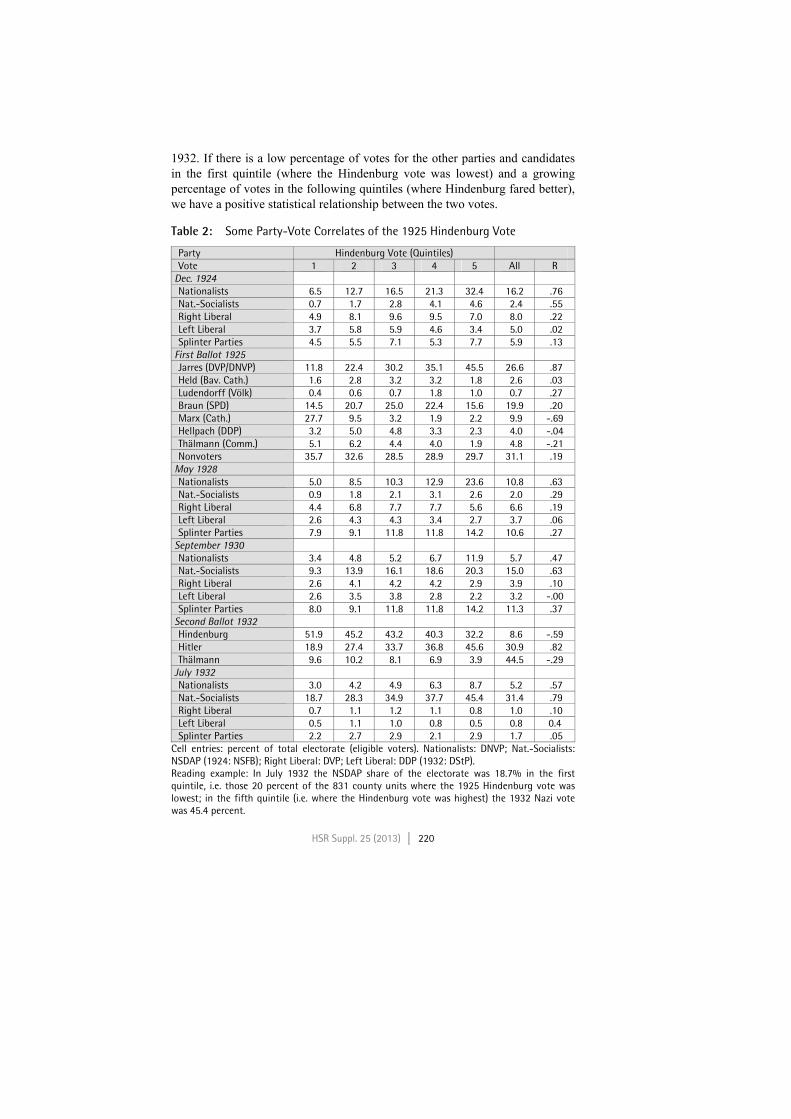
1932. If there is a low percentage of votes for the other parties and candidates in the first quintile (where the Hindenburg vote was lowest) and a growing percentage of votes in the following quintiles (where Hindenburg fared better), we have a positive statistical relationship between the two votes.

Table 2: Some Party-Vote Correlates of the 1925 Hindenburg Vote

Party Hindenburg Vote (Quintiles) Vote 1 2 3 4 5 All R

Dec. 1924 Nationalists 6.5 12.7 16.5 21.3 32.4 16.2 .76 Nat.-Socialists 0.7 1.7 2.8 4.1 4.6 2.4 .55 Right Liberal 4.9 8.1 9.6 9.5 7.0 8.0 .22 Left Liberal 3.7 5.8 5.9 4.6 3.4 5.0 .02 Splinter Parties 4.5 5.5 7.1 5.3 7.7 5.9 .13

First Ballot 1925 Jarres (DVP/DNVP) 11.8 22.4 30.2 35.1 45.5 26.6 .87 Held (Bav. Cath.) 1.6 2.8 3.2 3.2 1.8 2.6 .03 Ludendorff (Völk) 0.4 0.6 0.7 1.8 1.0 0.7 .27 Braun (SPD) 14.5 20.7 25.0 22.4 15.6 19.9 .20 Marx (Cath.) 27.7 9.5 3.2 1.9 2.2 9.9 -.69 Hellpach (DDP) 3.2 5.0 4.8 3.3 2.3 4.0 -.04 Thälmann (Comm.) 5.1 6.2 4.4 4.0 1.9 4.8 -.21 Nonvoters 35.7 32.6 28.5 28.9 29.7 31.1 .19

May 1928 Nationalists 5.0 8.5 10.3 12.9 23.6 10.8 .63 Nat.-Socialists 0.9 1.8 2.1 3.1 2.6 2.0 .29 Right Liberal 4.4 6.8 7.7 7.7 5.6 6.6 .19 Left Liberal 2.6 4.3 4.3 3.4 2.7 3.7 .06 Splinter Parties 7.9 9.1 11.8 11.8 14.2 10.6 .27

September 1930 Nationalists 3.4 4.8 5.2 6.7 11.9 5.7 .47 Nat.-Socialists 9.3 13.9 16.1 18.6 20.3 15.0 .63 Right Liberal 2.6 4.1 4.2 4.2 2.9 3.9 .10 Left Liberal 2.6 3.5 3.8 2.8 2.2 3.2 -.00 Splinter Parties 8.0 9.1 11.8 11.8 14.2 11.3 .37

Second Ballot 1932 Hindenburg 51.9 45.2 43.2 40.3 32.2 8.6 -.59 Hitler 18.9 27.4 33.7 36.8 45.6 30.9 .82 Thälmann 9.6 10.2 8.1 6.9 3.9 44.5 -.29

July 1932 Nationalists 3.0 4.2 4.9 6.3 8.7 5.2 .57 Nat.-Socialists 18.7 28.3 34.9 37.7 45.4 31.4 .79 Right Liberal 0.7 1.1 1.2 1.1 0.8 1.0 .10 Left Liberal 0.5 1.1 1.0 0.8 0.5 0.8 0.4 Splinter Parties 2.2 2.7 2.9 2.1 2.9 1.7 .05

Cell entries: percent of total electorate (eligible voters). Nationalists: DNVP; Nat.-Socialists: NSDAP (1924: NSFB); Right Liberal: DVP; Left Liberal: DDP (1932: DStP). Reading example: In July 1932 the NSDAP share of the electorate was 18.7% in the first quintile, i.e. those 20 percent of the 831 county units where the 1925 Hindenburg vote was lowest; in the fifth quintile (i.e. where the Hindenburg vote was highest) the 1932 Nazi vote was 45.4 percent.

HSR Suppl. 25 (2013) │ 221

The correlation coefficient therefore is positive in sign and rather high in mag-nitude. This is the case for the statistical association between the Hindenburg vote on the one hand, and the vote for the German National Party (DNVP) or the völkisch-Nazi coalition in the late-1924 parliamentary elections. A positive correlation also exists between the Hindenburg vote and the vote for the joint presidential candidate of the DNVP and the right-liberal DVP on the first ballot of 1925, Karl Jarres. In other words, the higher the Hindenburg vote of 1925 was in a county, the higher, on the average, the DNVP or Jarres vote was in that same county. The opposite applies to candidates who won relatively more votes in the first than in the subsequent Hindenburg quintiles, as is the case with Wilhelm Marx, his close competitor of 1925. The correlation coefficient still is comparatively high, but now of course negative in sign.

We thus find out that German Nationalists and the 1924 coalition of völk-isch and national-socialist splinters, as well as Jarres, displayed the same distri-bution of votes as Hindenburg did: they fared much better, on the average, in counties where Hindenburg was strong than in counties where Hindenburg was weak. For example, in the 165 counties of the first quintile, the Jarres vote amounted to not more than 11.8 percent of the electorate, while in the fifth quintile, the Jarres vote was up to 45.5 percent. In addition, there is a slight, curvilinear relationship between the Hindenburg vote and each of the follow-ing: turnout; the vote for the first-ballot candidate of the völkisch Right, Erich von Ludendorff; and, quite unexpectedly, the vote for the first ballot presiden-tial candidate of the Social Democrats, Otto Braun.

2.2 Some Ecological Regression Estimates of the “True” Voter Fluctuations to and from Paul von Hindenburg in 1925

It would be quite hazardous to interpret these findings in terms of individual or group relationships – to assume, that is, that all or most Hindenburg voters were necessarily former Jarres and DNVP voters. So-called ecological falla-cies, such as the erroneous assumption that the relationships of one level of analysis would be equivalent to the other, could (but by no means necessarily must) result from such a tacit assumption of congruence.3 To get somewhat better estimates of voter fluctuations, one has to take into consideration the development of the other parties or candidates as well. This is done by multiple ecological regression analysis – a powerful but somewhat dangerous statistical technique that bases its estimates on rather “strong” distributional premises such as linearity, non-contextuality of relationships, etc. Only if these premises

3 See Hayward R. Alker, Jr., “A Typology of Ecological Fallacies,” in Mattei Dogan and Stein

Rokkan, eds., Quantitative Ecological Analysis in the Social Sciences (Cambridge, Mass., 1969), 69-86. W. S. Robinson, “Ecological Correlations and the Behavior of Individuals,” American Sociological Review 40 (1950): 351-7.

HSR Suppl. 25 (2013) │ 222

are met by the data (which we cannot fully know) can the estimates of ecologi-cal regression equations be interpreted as “true” individual level fluctuations. If not, they still represent a good aggregate level estimate of the statistical rela-tionship between the development of the Hindenburg vote and the vote for other parties and candidates. Since we cannot completely know if all assump-tions of the method are really met, we should restrict our interpretation of the findings to differences of magnitude.4

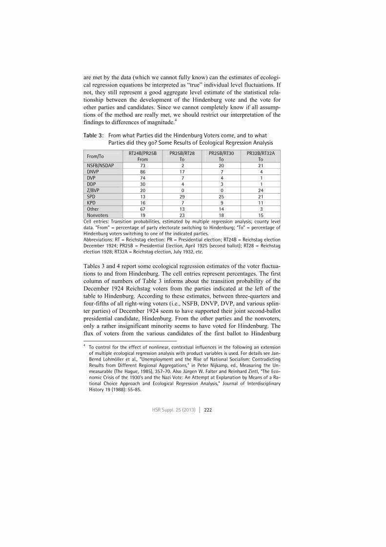
Table 3: From what Parties did the Hindenburg Voters come, and to what Parties did they go? Some Results of Ecological Regression Analysis

From/To RT24B/PR25B From

PR25B/RT28 To

PR25B/RT30 To

PR32B/RT32A To

NSFB/NSDAP 73 2 20 21 DNVP 86 17 7 4 DVP 74 7 4 1 DDP 30 4 3 1 Z/BVP 20 0 0 24 SPD 13 29 25 21 KPD 16 7 9 11 Other 67 13 14 3 Nonvoters 19 23 18 15

Cell entries: Transition probabilities, estimated by multiple regression analysis; county level data. “From” = percentage of party electorate switching to Hindenburg; “To” = percentage of Hindenburg voters switching to one of the indicated parties. Abbreviations: RT = Reichstag election: PR = Presidential election; RT24B = Reichstag election December 1924; PR25B = Presidential Election, April 1925 (second ballot); RT28 = Reichstag election 1928; RT32A = Reichstag election, July 1932, etc. Tables 3 and 4 report some ecological regression estimates of the voter fluctua-tions to and from Hindenburg. The cell entries represent percentages. The first column of numbers of Table 3 informs about the transition probability of the December 1924 Reichstag voters from the parties indicated at the left of the table to Hindenburg. According to these estimates, between three-quarters and four-fifths of all right-wing voters (i.e., NSFB, DNVP, DVP, and various splin-ter parties) of December 1924 seem to have supported their joint second-ballot presidential candidate, Hindenburg. From the other parties and the nonvoters, only a rather insignificant minority seems to have voted for Hindenburg. The flux of voters from the various candidates of the first ballot to Hindenburg 4 To control for the effect of nonlinear, contextual influences in the following an extension

of multiple ecological regression analysis with product variables is used. For details see Jan-Bernd Lohmöller et al., “Unemployment and the Rise of National Socialism: Contradicting Results from Different Regional Aggregations,” in Peter Nijkamp, ed., Measuring the Un-measurable (The Hague, 1985), 357-70. Also Jürgen W. Falter and Reinhard Zintl, “The Eco-nomic Crisis of the 1930’s and the Nazi Vote: An Attempt at Explanation by Means of a Ra-tional Choice Approach and Ecological Regression Analysis,” Journal of Interdisciplinary History 19 (1988): 55-85.

HSR Suppl. 25 (2013) │ 223

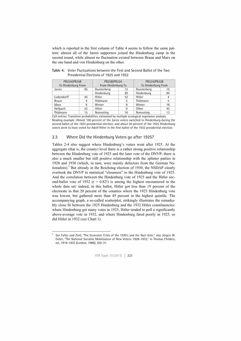
which is reported in the first column of Table 4 seems to follow the same pat-tern: almost all of the Jarres supporters joined the Hindenburg camp in the second round, while almost no fluctuation existed between Braun and Marx on the one hand and von Hindenburg on the other.

Table 4: Voter Fluctuations between the First and Second Ballot of the Two Presidential Elections of 1925 and 1932

PR25A/PR25B To Hindenburg From

PR25B/PR32A From Hindenburg To

PR32A/PR32B To Hindenburg From

Jarres 95 Duesterberg 12 Duesterberg 15 Hindenburg 20 Hindenburg 94 Ludendorff 45 Hitler 52 Hitler 4 Braun 4 Thälmann 5 Thälmann 5 Marx 9 Winter 0 Winter 16 Hellpach 22 Other 0 Other 45 Thälmann 15 Nonvoting 10 Nonvoting 13

Cell entries: Transition probabilities, estimated by multiple ecological regression analysis. Reading example: Almost 100 percent of the Jarres voters switched to Hindenburg during the second ballot of the 1925 presidential election; and about 50 percent of the 1925 Hindenburg voters seem to have voted for Adolf Hitler in the first ballot of the 1932 presidential election.

2.3 Where Did the Hindenburg Voters go after 1925?

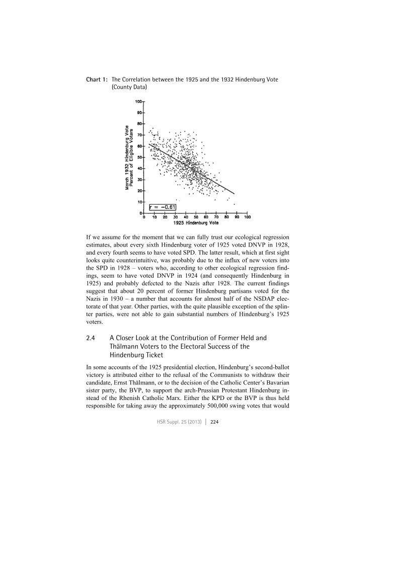
Tables 2-4 also suggest where Hindenburg’s voters went after 1925. At the aggregate (that is, the county) level there is a rather strong positive relationship between the Hindenburg vote of 1925 and the later vote of the DNVP; there is also a much smaller but still positive relationship with the splinter parties in 1928 and 1930 (which, in turn, were mainly defectors from the German Na-tionalists).5 But already in the Reichstag election of 1930, the NSDAP clearly overtook the DNVP in statistical “closeness” to the Hindenburg vote of 1925. And the correlation between the Hindenburg vote of 1925 and the Hitler sec-ond-ballot vote of 1932 (r = 0.82!) is among the highest encountered in the whole data set: indeed, in this ballot, Hitler got less than 19 percent of the electorate in that 20 percent of the counties where the 1925 Hindenburg vote was lowest, but gathered more than 45 percent in the highest quintile. The accompanying graph, a so-called scatterplot, strikingly illustrates the remarka-bly close fit between the 1925 Hindenburg and the 1932 Hitler constituencies: where Hindenburg got many votes in 1925, Hitler tended to poll a significantly above-average vote in 1932, and where Hindenburg fared poorly in 1925, so did Hitler in 1932 (see Chart 1).

5 See Falter and Zintl, “The Economic Crisis of the 1930’s and the Nazi Vote,” also Jürgen W.

Falter, “The National Socialist Mobilisation of New Voters: 1928-1933,” in Thomas Childers, ed., 1919-1933 (London, 1986), 202-31.

HSR Suppl. 25 (2013) │ 224

Chart 1: The Correlation between the 1925 and the 1932 Hindenburg Vote (County Data)

If we assume for the moment that we can fully trust our ecological regression estimates, about every sixth Hindenburg voter of 1925 voted DNVP in 1928, and every fourth seems to have voted SPD. The latter result, which at first sight looks quite counterintuitive, was probably due to the influx of new voters into the SPD in 1928 – voters who, according to other ecological regression find-ings, seem to have voted DNVP in 1924 (and consequently Hindenburg in 1925) and probably defected to the Nazis after 1928. The current findings suggest that about 20 percent of former Hindenburg partisans voted for the Nazis in 1930 – a number that accounts for almost half of the NSDAP elec-torate of that year. Other parties, with the quite plausible exception of the splin-ter parties, were not able to gain substantial numbers of Hindenburg’s 1925 voters.

2.4 A Closer Look at the Contribution of Former Held and Thälmann Voters to the Electoral Success of the Hindenburg Ticket

In some accounts of the 1925 presidential election, Hindenburg’s second-ballot victory is attributed either to the refusal of the Communists to withdraw their candidate, Ernst Thälmann, or to the decision of the Catholic Center’s Bavarian sister party, the BVP, to support the arch-Prussian Protestant Hindenburg in-stead of the Rhenish Catholic Marx. Either the KPD or the BVP is thus held responsible for taking away the approximately 500,000 swing votes that would

HSR Suppl. 25 (2013) │ 225

have assured victory to Wilhelm Marx. Putting the blame upon the Com-munists seems to me a bit farfetched: given the explicit enmity of this party toward the Weimar “capitalist state,” it would have been completely unrealistic to expect the KPD to support the candidate of the Weimar system. On the other hand, the BVP’s decision to support Hindenburg instead of Marx may indeed have been crucial. It is therefore worthwhile to analyze how many votes the Bavarian party’s decision might have cost the candidate of the Weimar coali-tion.

Table 5: The Correlation of the Held Vote with the Hindenburg and Marx Vote in Bavaria

1924B BVP Vote (Quintiles) 1925A Held Vote (Quintiles) 1st

Ballot 1 2 3 4 5 r 2nd Ballot 1 2 3 4 5 r

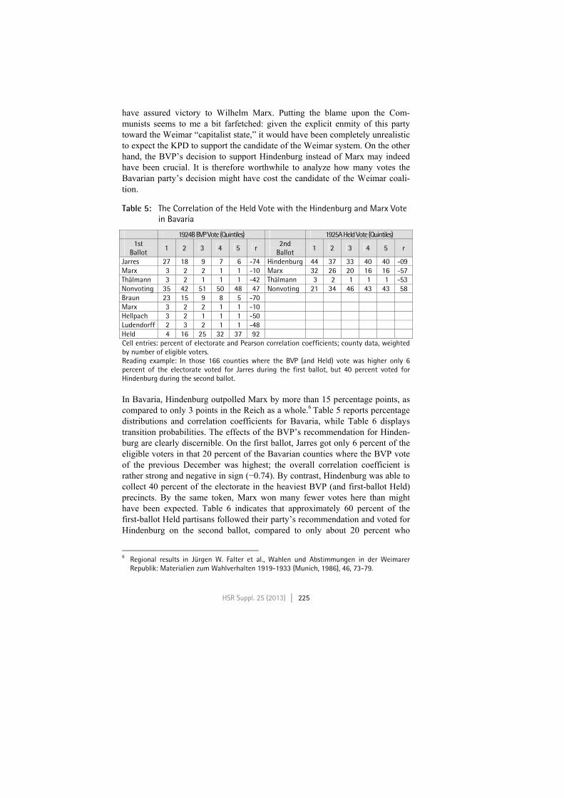
Jarres 27 18 9 7 6 -74 Hindenburg 44 37 33 40 40 -09 Marx 3 2 2 1 1 -10 Marx 32 26 20 16 16 -57 Thälmann 3 2 1 1 1 -42 Thälmann 3 2 1 1 1 -53 Nonvoting 35 42 51 50 48 47 Nonvoting 21 34 46 43 43 58 Braun 23 15 9 8 5 -70 Marx 3 2 2 1 1 -10 Hellpach 3 2 1 1 1 -50 Ludendorff 2 3 2 1 1 -48 Held 4 16 25 32 37 92 Cell entries: percent of electorate and Pearson correlation coefficients; county data, weighted by number of eligible voters. Reading example: In those 166 counties where the BVP (and Held) vote was higher only 6 percent of the electorate voted for Jarres during the first ballot, but 40 percent voted for Hindenburg during the second ballot. In Bavaria, Hindenburg outpolled Marx by more than 15 percentage points, as compared to only 3 points in the Reich as a whole.6 Table 5 reports percentage distributions and correlation coefficients for Bavaria, while Table 6 displays transition probabilities. The effects of the BVP’s recommendation for Hinden-burg are clearly discernible. On the first ballot, Jarres got only 6 percent of the eligible voters in that 20 percent of the Bavarian counties where the BVP vote of the previous December was highest; the overall correlation coefficient is rather strong and negative in sign (−0.74). By contrast, Hindenburg was able to collect 40 percent of the electorate in the heaviest BVP (and first-ballot Held) precincts. By the same token, Marx won many fewer votes here than might have been expected. Table 6 indicates that approximately 60 percent of the first-ballot Held partisans followed their party’s recommendation and voted for Hindenburg on the second ballot, compared to only about 20 percent who

6 Regional results in Jürgen W. Falter et al., Wahlen und Abstimmungen in der Weimarer

Republik: Materialien zum Wahlverhalten 1919-1933 (Munich, 1986), 46, 73-79.

HSR Suppl. 25 (2013) │ 226

switched to Marx. This would indeed imply that about half a million votes could be attributed to the BVP’s unfortunate recommendation. In the light of Hindenburg’s past political record, the BVP’s electoral policy may be charac-terized as shortsighted if not frivolous.

Table 6: Voting Transitions in Bavaria from the 1st to the 2nd Ballot of the 1925 Reichspräsident Elections (Ecological Regression Estimates)

First Ballot Second Ballot Nonvoting All First Ballot Hindenburg Marx

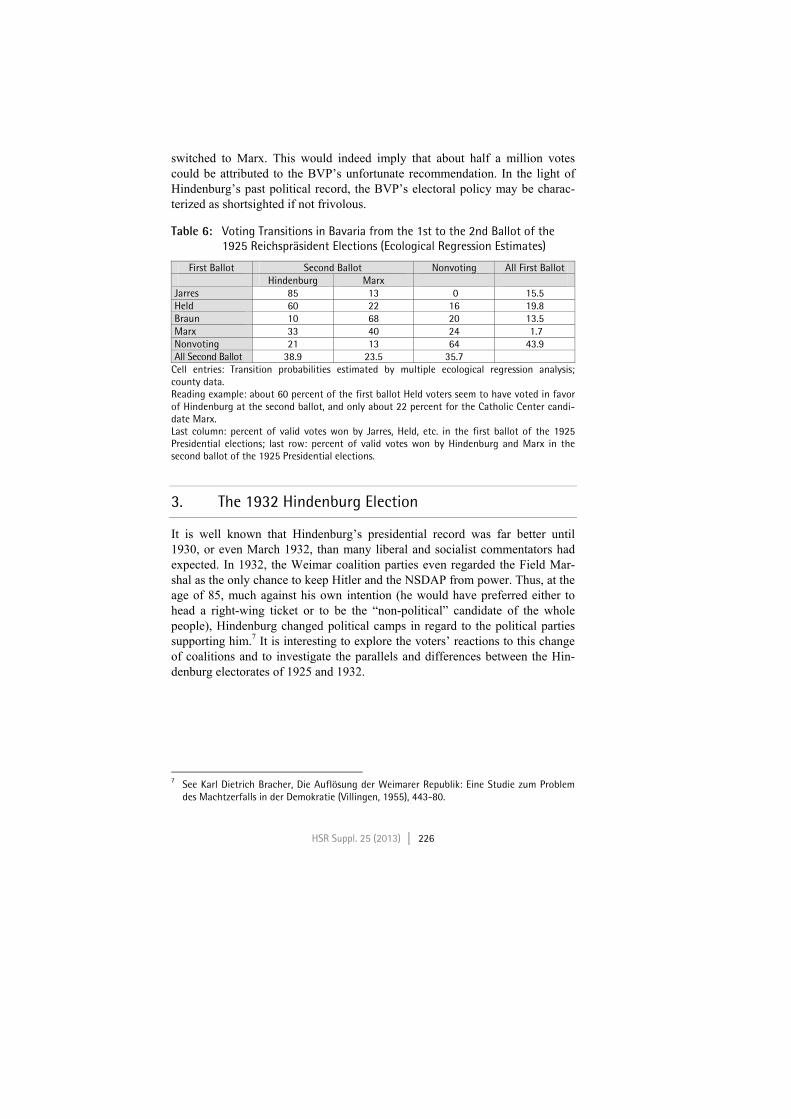
Jarres 85 13 0 15.5 Held 60 22 16 19.8 Braun 10 68 20 13.5 Marx 33 40 24 1.7 Nonvoting 21 13 64 43.9 All Second Ballot 38.9 23.5 35.7

Cell entries: Transition probabilities estimated by multiple ecological regression analysis; county data. Reading example: about 60 percent of the first ballot Held voters seem to have voted in favor of Hindenburg at the second ballot, and only about 22 percent for the Catholic Center candi-date Marx. Last column: percent of valid votes won by Jarres, Held, etc. in the first ballot of the 1925 Presidential elections; last row: percent of valid votes won by Hindenburg and Marx in the second ballot of the 1925 Presidential elections.

3. The 1932 Hindenburg Election

It is well known that Hindenburg’s presidential record was far better until 1930, or even March 1932, than many liberal and socialist commentators had expected. In 1932, the Weimar coalition parties even regarded the Field Mar-shal as the only chance to keep Hitler and the NSDAP from power. Thus, at the age of 85, much against his own intention (he would have preferred either to head a right-wing ticket or to be the “non-political” candidate of the whole people), Hindenburg changed political camps in regard to the political parties supporting him.7 It is interesting to explore the voters’ reactions to this change of coalitions and to investigate the parallels and differences between the Hin-denburg electorates of 1925 and 1932.

7 See Karl Dietrich Bracher, Die Auflösung der Weimarer Republik: Eine Studie zum Problem

des Machtzerfalls in der Demokratie (Villingen, 1955), 443-80.

HSR Suppl. 25 (2013) │ 227

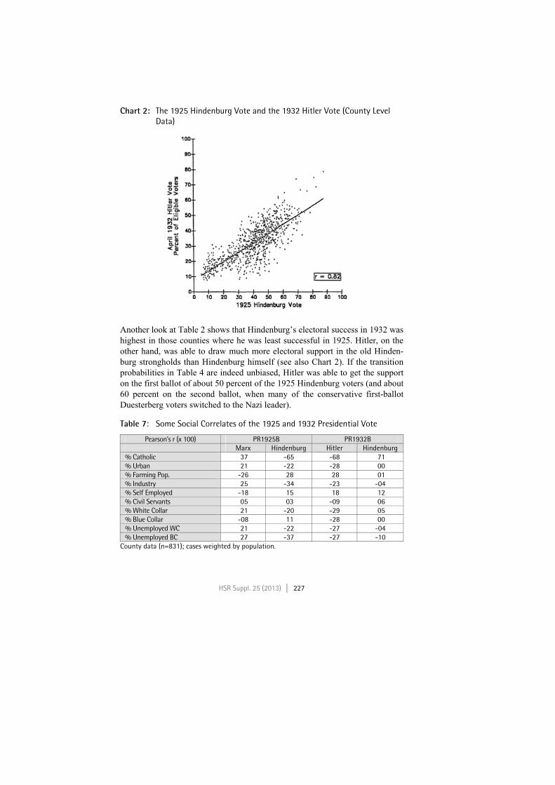
Chart 2: The 1925 Hindenburg Vote and the 1932 Hitler Vote (County Level Data)

Another look at Table 2 shows that Hindenburg’s electoral success in 1932 was highest in those counties where he was least successful in 1925. Hitler, on the other hand, was able to draw much more electoral support in the old Hinden-burg strongholds than Hindenburg himself (see also Chart 2). If the transition probabilities in Table 4 are indeed unbiased, Hitler was able to get the support on the first ballot of about 50 percent of the 1925 Hindenburg voters (and about 60 percent on the second ballot, when many of the conservative first-ballot Duesterberg voters switched to the Nazi leader).

Table 7: Some Social Correlates of the 1925 and 1932 Presidential Vote

Pearson's r (x 100) PR1925B PR1932B Marx Hindenburg Hitler Hindenburg

% Catholic 37 -65 -68 71 % Urban 21 -22 -28 00 % Farming Pop. -26 28 28 01 % Industry 25 -34 -23 -04 % Self Employed -18 15 18 12 % Civil Servants 05 03 -09 06 % White Collar 21 -20 -29 05 % Blue Collar -08 11 -28 00 % Unemployed WC 21 -22 -27 -04 % Unemployed BC 27 -37 -27 -10

County data (n=831); cases weighted by population.

HSR Suppl. 25 (2013) │ 228

From the perspective of voter fluctuations, Hindenburg seems to have lost his old constituency. He was reinstated in office by his former opponents, the followers of the Catholic Center Party, the Social Democrats, and the few re-maining left-liberals of the DDP/ DStP.

The social correlates of the vote of the two main contenders of 1925 and 1933, as displayed in Table 7, reveal the radical rearrangement undergone by the Hindenburg voting coalition. In 1925, the Hindenburg vote was lower in predominantly Catholic, in urban, industrialized districts, and in regions where unemployment was above average. By contrast, the Hindenburg vote of 1932 increased with the number of Catholics and self-employed in the district. And Hitler’s constituency of 1932, like Hindenburg’s of 1925, was located in pre-dominantly Protestant counties, in rural areas, and in districts with lower than average unemployment rates.8

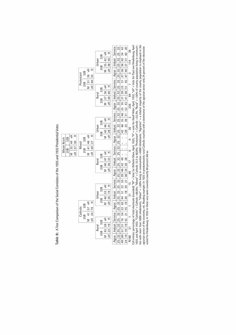
The information presented in Table 7 is bivariate in character: only two var-iables are compared at one time. The real world, however, is different: nobody is only Catholic or Protestant, only young or old, only farmer or blue-collar worker. The same is true for the territorial units which form the basis of the analysis: county units are Catholic and rural and predominantly agrarian, etc. To account for this mix of social characteristics, one may combine some of the most important explanatory properties of the counties in a tree comparison (Table 8). In order to construct such a “tree,” we first divide the 831 county units of the Reich into three subgroups according to the percentage of Catholics living in these counties (religious denomination is by far the most important predictor of the Hitler and Hindenburg vote in 1932!). For these three sub-groups of counties, we calculate the average percentage of Hindenburg, Hitler, and Marx voters. In the next step the three denominational county classes are then divided according to their degree of urbanization. Again the average per-centage of Hindenburg, Hitler, and Marx voters is calculated for each of the resulting six groups. We thus find, for example, that the Hindenburg vote was far below average in rural Catholic areas in 1925 (23 percent); in 1932, howev-er, Hindenburg was able in these very same counties to mobilize 59 percent of the eligible voters, while Adolf Hitler was able to win only 19 percent of the electorate in this branch of our tree.

8 Quite unexpectedly the Nazis fared much better in districts with low levels of unemploy-

ment. On the average, the unemployed seem to have been clearly underrepresented among Nazi voters. See Jürgen W. Falter, “Unemployment and the Radicalisation of the German Electorate 1928-1933: An Aggregate Data Analysis with Special Emphasis on the Rise of National Socialism,” in Peter Stachura, ed., Unemployment and the Great Depression in Weimar Germany (Houndsmill/London, 1986), 187-208, and Jürgen W. Falter, Hitlers Wähler (Munich, 1991), 292-314.

Tabl

e 8:

A Tr

ee C

ompa

rison

of t

he S

ocia

l Cor

rela

tes o

f the

192

5 an

d 19

32 P

resid

entia

l Vot

es

Who

le R

eich

25

B 32

B

M

vH

35

37

44

30

vH H

Cath

olic

M

ixed

Pr

otes

tant

25

B 32

B

25

B 32

B

25

B 32

B

M

vH

41 2457 19

vH H

M

vH

41

30

46

27

vH H

M

vH

31 4439 34

vH H

Ru

ral

Urb

an

Rura

l

U

rban

Ru

ral

Urb

an

25B

32B

25B

32B

25B

32B

25B

32B

25B

32B

25B

32B

M

vH42 23

59 19vH H

M

vH40 26

53 19vH H

M

vH40 36

47 33vH H

M

vH42 28

46 25vH H

M

vH27 49

36 40vH H

M

vH35 38

42 30vH H

Agra

r In

dust

Serv

ice

Agra

r In

dust

Serv

ice

Agra

r In

dust

Serv

ice

Agra

r In

dust

Serv

ice

Agra

r In

dust

Serv

ice

Agra

r In

dust

Serv

ice

25

3225

3225

3225

3225

3225

3225

3225

3225

32

25

3225

3225

3225

3225

3225

3225

3225

3225

3240

24

60 19

51 1951 19

16 4254 21

22 3562 19

44 2051 18

33 3955 21

39 3846 34

42 3049 28

- - - -

- - - -

42 2846 25

35 3946 31

25 5335 43

31 4139 36

23 5131 45

27 4736 40

36 3742 31

34 4042 30

N18

8 21

1

1 31

15

49

17

0

0 36

2

226

84

1 3

114

38

Cell

entr

ies:

perc

enta

ge o

f tot

al e

lect

orat

e (ro

unde

d). “

M” =

Vot

e fo

r Wilh

elm

Mar

x, Ap

ril, 1

925;

“H” =

vot

e fo

r Ado

lf Hi

tler,

April

, 193

2; “v

H” =

Vot

e fo

r Pau

l von

Hin

denb

urg,

Apr

il 19

25 a

nd A

pril

1932

. “Ca

thol

ic” =

Cat

holic

>66

.6%

; “M

ixed

” = C

atho

lic 3

3.3

to 6

6.6%

; “Pr

otes

tant

” = C

atho

lic <

33.3

%. “

Rura

l” =

<50%

of c

ount

y po

pula

tion

livin

g in

com

mun

i-tie

s w

ith m

ore

than

500

0 in

habi

tant

s; “U

rban

” =

>50%

livi

ng in

com

mun

ities

>50

00 in

habi

tant

s. “A

grar

ian”

= a

rel

ativ

e m

ajor

ity o

f th

e co

unty

pop

ulat

ion

is em

ploy

ed in

the

ag

raria

n se

ctor

of t

he e

cono

my,

etc.

Read

ing

exam

ple:

In 1

925

in p

redo

min

atel

y ru

ral C

atho

lic c

ount

ies w

ith a

dom

inan

ce o

f the

agr

aria

n se

ctor

onl

y 24

per

cent

of t

he e

lect

orat

e

vote

d fo

r Hin

denb

urg;

in 1

932

in th

ese

very

sam

e co

untie

s exa

ctly

60

perc

ent d

id so

.

HSR Suppl. 25 (2013) │ 230

In the next and final step, the resulting six county classes are again divided into three sub-classes each, according to the prevalent economic sector, so that we are now looking at 18 different county categories which are socially and politi-cally more homogeneous than the less differentiated branches of the tree above this last level. We then determine the share of the vote in each of the eighteen branches for the three main contenders of the two elections under considera-tion.9

While space constraints prohibit a detailed description, one can readily see from the “tree” that the Hindenburg voting coalition underwent a radical change: the distribution of Hindenburg votes in 1932 is much closer to that of the Marx vote of 1925 than to the first Hindenburg vote. Likewise, the Hitler vote of 1932 closely matches the Hindenburg vote of 1925: in those socially defined subgroups where Hindenburg’s showing was strong in 1925, Hitler gathered an above-average share of the votes in 1932, and vice versa. From this perspective, the conservative and right-wing voter coalition that brought Hin-denburg into power in the first Weimar presidential election may indeed be described as the harbinger of the electoral triumphs of the NSDAP of 1932 and 1933. It therefore may be interpreted as the first effective gathering of the anti-republican forces that would later bring the Weimar Republic to an end.10

4. Did Indeed Many Thälmann Voters of the First Ballot Vote for Hitler in the Second Ballot of the 1932 Presidential Election?

It is often suggested that the increase in Hitler’s constituency (about 2 million votes) during the second ballot of the 1932 presidential election may have been largely due to defections from the Communist leader Ernst Thälmann, who lost about 1.2 million votes. This hypothesis, which is based mostly on local im-pressionistic evidence (the proverbial Communist tavern which changed colors overnight), is rooted in the widespread conviction that ultimately the totalitari-an extremes were not so terribly far apart and that the step from the Com-munists to the Nazis was much more readily taken than ideology or propaganda might lead one to expect. This idea of the proximity of the extremes finds addi-

9 Analogous “trees” for all major parties and Weimar elections are presented in Jürgen W.

Falter et al., Wahlen und Abstimmungen in der Weimarer Republik, 194-203. 10 In fact in the multivariate model the Hindenburg vote of 1925 (which in turn may be inter-

preted as a proximity measure of a right-wing political tradition) is the second best predic-tor of the Nazi vote (after the religious composition of the counties)! See Jürgen W. Falter and Dirk Hänisch, “Die Anfälligkeit von Arbeitern gegenüber der NSDAP bei den Reichstags-wahlen 1928-1933,” Archiv für Sozialgeschichte 26 (1986): 179-216, Reprint in this HSR Supplement.

HSR Suppl. 25 (2013) │ 231

tional theoretical endorsement in the conviction that many, if not most, of Hit-ler’s and Thälmann’s followers were unpolitical, socially uprooted products of mass society, so-called protest voters who could easily be seduced by unrealis-tic promises and who therefore fell prey to the totalitarian temptations of the time.11 However, little quantitative evidence has ever been provided that would either prove or disprove this transition hypothesis.

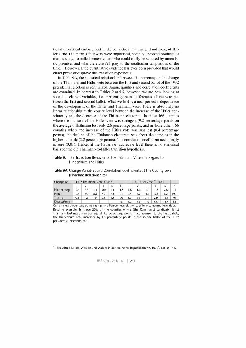
In Table 9A, the statistical relationship between the percentage point change of the Thälmann and Hitler vote between the first and second ballot of the 1932 presidential election is scrutinized. Again, quintiles and correlation coefficients are examined. In contrast to Tables 2 and 5, however, we are now looking at so-called change variables, i.e., percentage-point differences of the vote be-tween the first and second ballot. What we find is a near-perfect independence of the development of the Hitler and Thälmann vote. There is absolutely no linear relationship at the county level between the increase of the Hitler con-stituency and the decrease of the Thälmann electorate. In those 166 counties where the increase of the Hitler vote was strongest (9.2 percentage points on the average), Thälmann lost only 2.6 percentage points; and in those other 166 counties where the increase of the Hitler vote was smallest (0.4 percentage points), the decline of the Thälmann electorate was about the same as in the highest quintile (2.2 percentage points). The correlation coefficient accordingly is zero (0.01). Hence, at the (bivariate) aggregate level there is no empirical basis for the old Thälmann-to-Hitler transition hypothesis.

Table 9: The Transition Behavior of the Thälmann Voters in Regard to Hindenburg and Hitler

Table 9A: Change Variables and Correlation Coefficients at the County Level (Bivariate Relationships)

Change of 1932 Thälmann Vote (Quint.) 1932 Hitler Vote (Quint.) 1 2 3 4 5 r 1 2 3 4 5 r Hindenburg 2.6 2.2 1.4 0.9 1.5 12 1.5 1.6 1.0 1.2 2.5 11 Hitler 2.6 5.0 5.3 4.7 4.6 01 0.4 2.7 4.2 5.8 9.2 100 Thälmann -0.5 -1.2 -1.9 -2.8 -4.8 100 -2.2 -3.4 -3.1 -2.9 -2.6 01 Duesterberg - - - - - -16 -1.9 -3.3 -4.5 -6.6 -12.7 -83

Cell entries: percentage point change and Pearson correlation coefficients, county level data. Reading example: In those 20% of the counties where (the Communist candidate) Ernst Thälmann lost most (=an average of 4.8 percentage points in comparison to the first ballot), the Hindenburg vote increased by 1.5 percentage points in the second ballot of the 1932 presidential elections, etc.

11 See Alfred Milatz, Wahlen und Wähler in der Weimarer Republik (Bonn, 1965), 138-9, 141.

HSR Suppl. 25 (2013) │ 232

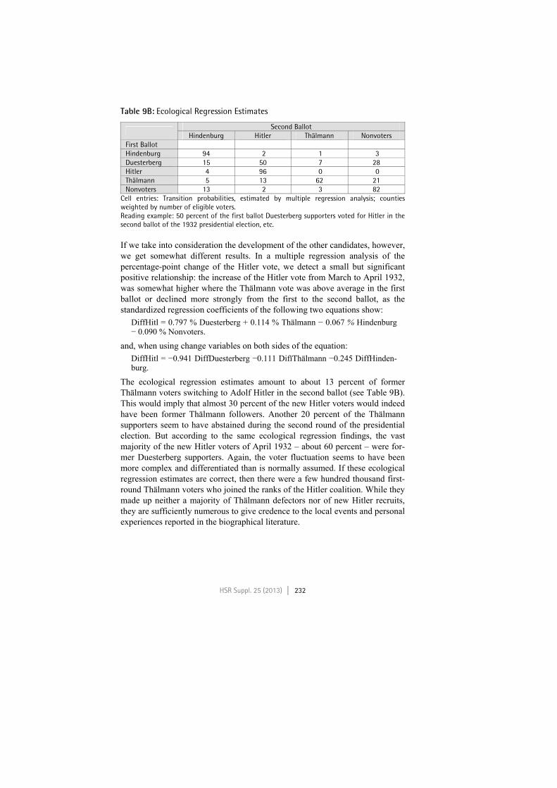
Table 9B: Ecological Regression Estimates

Second Ballot Hindenburg Hitler Thälmann Nonvoters

First Ballot Hindenburg 94 2 1 3 Duesterberg 15 50 7 28 Hitler 4 96 0 0 Thälmann 5 13 62 21 Nonvoters 13 2 3 82

Cell entries: Transition probabilities, estimated by multiple regression analysis; counties weighted by number of eligible voters. Reading example: 50 percent of the first ballot Duesterberg supporters voted for Hitler in the second ballot of the 1932 presidential election, etc. If we take into consideration the development of the other candidates, however, we get somewhat different results. In a multiple regression analysis of the percentage-point change of the Hitler vote, we detect a small but significant positive relationship: the increase of the Hitler vote from March to April 1932, was somewhat higher where the Thälmann vote was above average in the first ballot or declined more strongly from the first to the second ballot, as the standardized regression coefficients of the following two equations show:

DiffHitl = 0.797 % Duesterberg + 0.114 % Thälmann − 0.067 % Hindenburg − 0.090 % Nonvoters.

and, when using change variables on both sides of the equation:

DiffHitl = −0.941 DiffDuesterberg −0.111 DifïThälmann −0.245 DiffHinden-burg.

The ecological regression estimates amount to about 13 percent of former Thälmann voters switching to Adolf Hitler in the second ballot (see Table 9B). This would imply that almost 30 percent of the new Hitler voters would indeed have been former Thälmann followers. Another 20 percent of the Thälmann supporters seem to have abstained during the second round of the presidential election. But according to the same ecological regression findings, the vast majority of the new Hitler voters of April 1932 – about 60 percent – were for-mer Duesterberg supporters. Again, the voter fluctuation seems to have been more complex and differentiated than is normally assumed. If these ecological regression estimates are correct, then there were a few hundred thousand first-round Thälmann voters who joined the ranks of the Hitler coalition. While they made up neither a majority of Thälmann defectors nor of new Hitler recruits, they are sufficiently numerous to give credence to the local events and personal experiences reported in the biographical literature.