centers of complex networks - bioinf.uni-leipzig.de

Centers of Complex Networks

Stefan Wuchty†,‡ and Peter F. Stadler#,¶,§

†European Media Laboratory, Villa Bosch, Schloss-Wolfsbrunnenweg 33, D-69118Heidelberg, Germany

‡Department of Physics, 225 Nieuwland Science Hall, University of Notre Dame,Notre Dame, IN 46556, U.S.A.

∗,#Institut fur Theoretische Chemie und Molekulare Strukturbiologie, UniversitatWien, Wahringerstraße 17, A-1090 Wien, Austria

¶Lehrstuhl fur Bioinformatik, Institut fur Informatik, Universitat Leipzig,Kreuzstraße 7b, D-04103 Leipzig, Germany

§The Santa Fe Institute, 1399 Hyde Park Road, Santa Fe, NM 87501, USA

∗Address for correspondence.

Tel: ++43 1 4277 52737, Fax: ++43 1 4277 52793, Email: [email protected]

Abstract. The central vertices in complex networks are of particular interest be-cause they might play the role of organizational hubs. Here, we consider three differ-ent geometric centrality measures, eccentricity, status, and centroid value, that wereoriginally used in the context of resource placement problems. We show that thesequantities lead to useful descriptions of the centers of biological networks which often,but not always, correlate with a purely local notion of centrality such as the vertexdegree. We introduce the notion of local centers as local optima of a centrality value“landscape” on a network and discuss briefly their role.

1

S. Wuchty, P.F. Stadler: Centers of Complex Networks 2

1. Introduction

Complex networks occur in diverse areas from metabolic and gene regulation networksin each cell, food webs in ecology, transportation networks, economic interactions andthe organization of the internet, just to mention a few examples. Starting with theseminal paper by (Watts & Strogatz, 1998), it has been recognized that these real lifenetwork differ qualitatively from the classical random graph models (Erdos & Renyi,1960; Bollobas, 1985) by the so-called small-world property: while the graphs arevery sparse on average, the mutual distances between their vertices are neverthelessmuch shorter than expected.

The recent review by (Albert & Barabasi, 2002) indicates that current research focuseson the one hand evolving graphs with various preferential attachment rules and,on the other hand, on characterizing new empirically determined graphs in termsof a small number of parameters, in particular their degree distribution, clusteringcoefficient, and average path length. The vertex degree is typically used as a measureof centrality in these networks. In the graph evolution models, high vertex degreesusually indicate “old” vertices. (Fell & Wagner, 2000; Wagner & Fell, 2000) indeedshow that the metabolites with the highest connectivity are part of the oldest “core”metabolism.

It is a bit surprising, however, that classical graph-theoretical properties of such largereal-life networks so far have not been studied systematically, although at least someof them are easily within the reach of present-day computer facilities. In this con-tribution, we consider three notions of centrality that were originally designed forresource location problems. As such, these measure seem to be particularly appropri-ate for the study of metabolic and signaling networks, which after all have probablyevolved to solve the tasks of efficiently allocating resources to required metabolitesand of controlling a cell’s biochemistry with as little time delay as possible.

This contribution is organized as follows: In section 2 we provide some backgroundon the global structure of networks and introduce centrality measures and their basicproperties. These measures are compared in the subsequent section, where we alsointroduce the notion of a local center in a graph. Applications to three different typesof biological networks are discussed briefly in section 4, namely metabolic networks,protein interaction networks, and protein domain networks.

2. Network Structure

2.1. Basic Definitions. A network is conveniently modeled as a graph G whichconsists of a set V of vertices and a set E of edges which we regard as un-ordered pairsof distinct vertices. Hence we consider only simple undirected graphs in the languageof (Berge, 1985). A path in G is an alternating sequence (x0, e1, x1, . . . , e`, x`) ofvertices and edges, where the ei = {xi−1, xi} are the edges connecting subsequentvertices. The length of a path is its number edges. The set of neighbors of x isdenoted by ∂{x} = {y ∈ V |{x, y} ∈ E}.


The degree of a vertex x is the number of edges that contain x, i.e., the number ofneighbors of x:

deg(x) = |{e ∈ E|x ∈ e}| = |{y ∈ V | {x, y} ∈ E}| = |∂{x}| , (1)

where |A| denotes the cardinality (number of elements) of the set A. Equivalently,we may define deg(x) as the number of edges incident with x.

The distance d(x, y) is the length of the shortest path in G connecting x with y. Ifa path connecting x and y does not exist we set d(x, y) = ∞. Thus, the graph G isconnected if and only if d(x, y) is finite for all x, y ∈ V .

We remark that our approach can trivially be extended to weighted graphs. So,simply define deg(x) as the sum of the weight of the edges that contain x and definethe length of a path as the sum of the weights of each edges.

2.2. Degree Distributions. (Amaral et al., 2000) showed that there are (at least)three structurally different classes of networks that are distinguished by the distribu-tion P (k) of the vertex degrees k = deg(x):

(a) Single-Scale Networks with a sharp distribution of vertex degrees exhibitingexponential or Gaussian tails. This class includes also the Erdos-Renyi modelof uncorrelated random graphs (Erdos & Renyi, 1960; Bollobas, 1985).

(b) Scale-Free Networks with a power law distribution P (d) ∼ d−γ. A simplemodel for this type of networks was introduced recently by Barabasi et al.(Barabasi & Albert, 1999; Barabasi et al., 1999). Metabolic networks (Wagner& Fell, 2000; Jeong et al., 2000) and food-webs (Montoya & Sole, 2002) belongto this class.

(c) Broad-Scale Networks for which P (d) has a power-law regime followed by asharp cut-off, e.g. exponential or Gaussian decay of the tail. An example isthe movie-actor network described in (Watts, 1999)

The Erdos-Renyi model (ER) (Erdos & Renyi, 1960) assumes a fixed number n = |V |of vertices and assigns edges independently with a certain probability p. For detailssee the book by (Bollobas, 1985). In many cases, ER random graphs turn out thebe quite different from a network of interest. The Watts-Strogatz (SW) (Watts &Strogatz, 1998) model of small-world networks starts with a deterministic graph,usually a circular arrangement of vertices in which each vertex is connected to k

nearest neighbors on each side. Subsequently, edges are “rewired” (in the originalversion) or added (Newman & Watts, 1999; Newman et al., 2000) with probability p.Both ER and SW graphs exhibit an approximately Gaussian degree distributions.

The other extreme is the scale-free model (BA) (Barabasi & Albert, 1999; Barabasiet al., 1999) with a degree distribution of the form P (d) ∼ k−3. Starting from asmall core graph, at each time step a vertex is added together with m edges that areconnected to each previously present vertex k with probability

Π(k) = d(k)/

∑

k

d(k) , (2)

where d(k) is the degree of vertex k. A recent extension of the model allows thetuning of the scaling exponent γ in the range 2 ≤ γ ≤ 3 (Albert & Barabasi, 2000a).


The vertex degrees are an intrinsically local characterization of a graph. Consequently,they allow a meaningful interpretation only when the graph is a typical instance of aknown statistical ensemble such as the ER model or the BA model.

It is therefore necessary to consider additional characteristics of G that are preferablynot closely related to the degree distribution. A quantity that is commonly used inthe literature on the small-world networks is the clustering coefficient that measureshow close the neighborhood of a each vertex comes on average to being a completesubgraph (clique) (Herzel, 1998; Barrat & Weigt, 2000; Watts & Strogatz, 1998).Again, this measure is intrinsically local. A more global measure is the average length`(G) of a path between two vertices, see e.g. for an extensive discussion (Newmanet al., 2000). The distribution of short cycles, i.e., detours, may be regarded as anintermediate case (Gleiss et al., 2001).

2.3. Geometric Centrality. Geometric notions of centrality are closely linked tofacility location problems. Suppose, we are given a graph G representing, say, a trafficnetwork. We may then ask questions such as the following:

(A) What is the optimal location of a hospital such that the worst case responsetime of an ambulance is minimal?

(B) What is the optimal location of a shopping mall so that the average drivingtime to the mall is minimal?

(C) What is the optimal location of a shop if customers buy at the nearest shop,and there will be a competitor placing its shop after we have placed ours?

These three classical facility local problems can be recast as optimization problemsbased on the distance matrix D = (d(x, y)) of G. Their solutions define three dif-ferent notions of “central” vertices. The distance matrix D can be computed ratherefficiently e.g. using Dijkstra’s algorithm with time complexity O(|V |2 ln |V |), see e.g.(Cormen et al., 1990).

The excentricity of a vertex x in G and the radius ρ(G), respectively, are defined as

e(x) = maxy∈V

d(x, y) and ρ(G) = minx∈V

e(x) (3)

The center of G is the set

C(G) = {x ∈ V |e(x) = ρ(G)} . (4)

C(G) is the center to the “emergency facility local problem” (A) which is alwayscontained in a single block of G (Harary & Norman, 1953).

The status d(x) of a vertex (Harary, 1959) and the status σ(G) of the graph G,respectively, are defined as

d(x) =∑

y∈V

d(x, y) and σ(G) = minx∈V

d(x) . (5)

The median (Slater, 1980) of G is the set

M(G) = {x ∈ V |d(x) = σ(G)} . (6)

The median is the solution of the “service facility location problem” (B). Both thecenter and the median of a graph were already considered by (Jordan, 1869). Instead


of the status, one may of course use the average distance `(x) of a vertex from x.Clearly, d(x) = (|V | − 1)`(x). The Wiener index (Wiener, 1947) is

W (G) =1

2

∑

x∈V

d(x) =1

2

∑

x,y∈V

d(x, y) =

(

n

2

)

`(G) , (7)

where `(G) is the mean path length in G. It provides an important characteristic ofmolecular graphs. For details, see (Gutman et al., 1996).

For any pair of distinct vertices u, v ∈ V , u 6= v, define

Vxy = {w ∈ V |d(x, w) < d(y, w)} , (8)

i.e., Vuv is the set of vertices that are closer to u than to v. The competitive locationproblem (C), which was first considered by (Slater, 1975), is then solved by thevertices x that maximize |Vxy| − |Vyx| over all possible locations of the competitor y.The following identity

d(x) + |Vxy| = d(y) + |Vyx| (9)

holds for all connected graphs (Entringer et al., 1976). Following (Slater, 1975) wedefine centroid value of a vertex and the graph G itself as

f(x) = d(x) − miny 6=x

d(y) and ϕ(G) = minx∈V

f(x) . (10)

The centroid of G is the set

Z(G) = {x ∈ V |f(x) = ϕ(G)} . (11)

We have inverted the sign of f(x) compared to the discussion in Slater’s work (Slater,1999) as we prefer the centrality measure f(x) to be minimal at the most centralvertices in analogy to d(x) and e(x).

The mutual location of the three types of “central” vertices is of obvious interest.The median M(G) and the centroid Z(G) are always contained in the same block ofa connected graph G (Smart & Slater, 1999). Both, the center and the centroid mayserve as the root of a distance preserving spaning tree (Barefoot et al., 1997).

The centroid value f(x) may, perhaps surprisingly, become 0 or even negative. Ifthis is the case, then d(x) = miny d(y) = σ(G). It follows that f(x) < 0 for at mostone vertex x∗, in which case d(x∗) is the unique minimum of d(x), hence Z(G) =M(G) = {x∗}. If f is non-negative then f(x) = 0 iff d(x) is minimal and there are atleast two distinct vertices minimizing d. Again we have Z(G) = M(G). Conversely,if ϕ(G) > 0 then the minima of d(x) do not minimize f(x) and hence median andcentroid are disjoint. Such graphs are called secure graphs. It is shown in (Slater,1976) that there are no secure graphs with |V | < 9 vertices. An example with |V | ≥ 9is given (Smart & Slater, 1999, Fig.4).

It is shown in (Smart & Slater, 1999) that C(G), M(G), and Z(G) may be pairwisedisjoint and even separated by arbitrary distances if G is large enough (Slater, 1999).

A slightly different, much less studied notion of centrality is introduced in (Nieminen,1984). An induced subgraph H of G is convex if it contains a shortest path (in G)between any two of its vertices. A branch of G at a vertex x is a maximal convexinduced subgraph that does not contain x. The branch weight b(x) is the maximum


number of vertices in a branch of G at x. The branches of a tree T at a vertex x

are thus the connected components of the forest obtained by deleting the vertex x.The convex center or branch weight center B(G) is the set of vertices that minimizeb(x). (Zelinka, 1968) showed that for any tree T the convex center and the mediancoincide. We shall not consider the branch weight center in this contribution becausethere does not seem to be a convenient way to compute b(x) in large graphs.

Betweenness centrality (Freeman, 1977) is a distant relative of the resource placementcentralities discussed above. Originally designed to measure a person’s influence in asociety, it is quantified in terms of the number of shortest paths that run through agiven vertex. Most recently, a classification of scale-free networks based on the scalingof betweenness centrality has been proposed (Goh et al., 2002). A comparison of thismeasure with resource placement centralities will be described elsewhere.

3. Properties of Centrality Measures

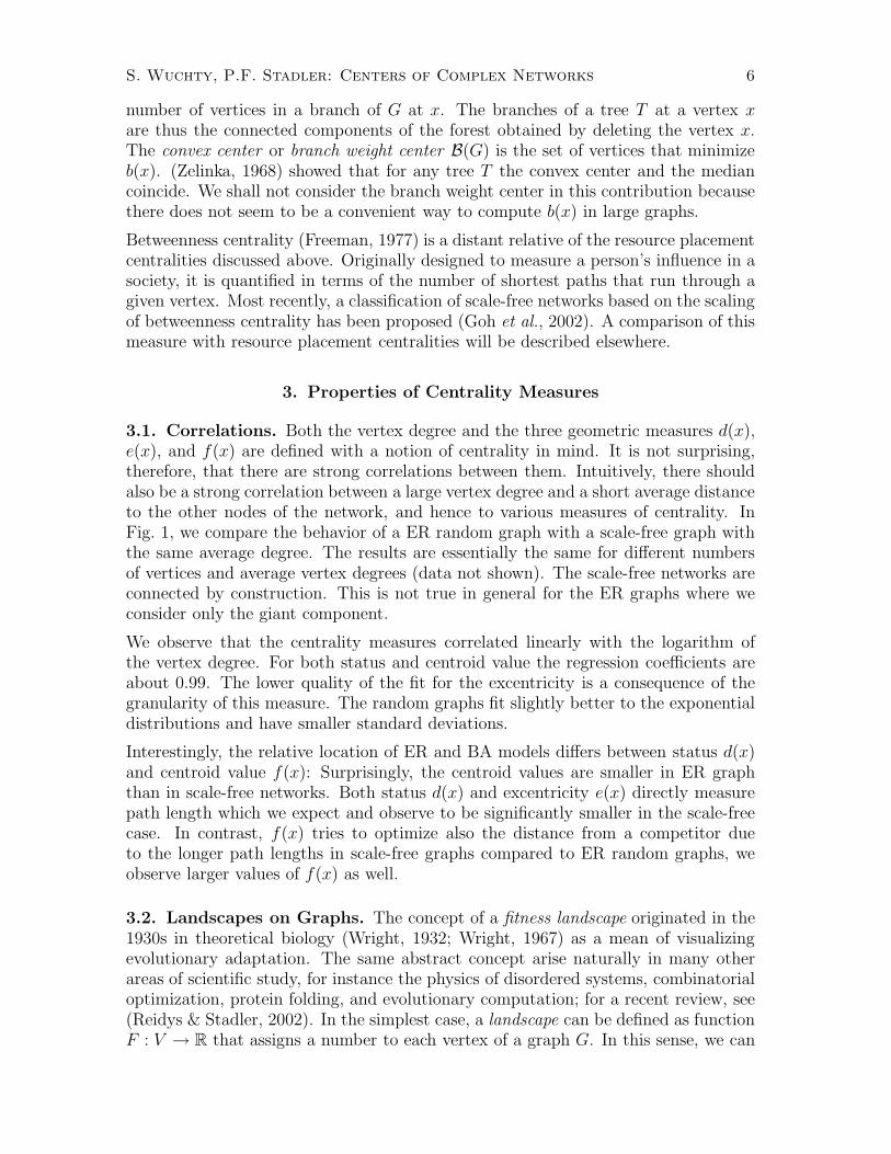
3.1. Correlations. Both the vertex degree and the three geometric measures d(x),e(x), and f(x) are defined with a notion of centrality in mind. It is not surprising,therefore, that there are strong correlations between them. Intuitively, there shouldalso be a strong correlation between a large vertex degree and a short average distanceto the other nodes of the network, and hence to various measures of centrality. InFig. 1, we compare the behavior of a ER random graph with a scale-free graph withthe same average degree. The results are essentially the same for different numbersof vertices and average vertex degrees (data not shown). The scale-free networks areconnected by construction. This is not true in general for the ER graphs where weconsider only the giant component.

We observe that the centrality measures correlated linearly with the logarithm ofthe vertex degree. For both status and centroid value the regression coefficients areabout 0.99. The lower quality of the fit for the excentricity is a consequence of thegranularity of this measure. The random graphs fit slightly better to the exponentialdistributions and have smaller standard deviations.

Interestingly, the relative location of ER and BA models differs between status d(x)and centroid value f(x): Surprisingly, the centroid values are smaller in ER graphthan in scale-free networks. Both status d(x) and excentricity e(x) directly measurepath length which we expect and observe to be significantly smaller in the scale-freecase. In contrast, f(x) tries to optimize also the distance from a competitor dueto the longer path lengths in scale-free graphs compared to ER random graphs, weobserve larger values of f(x) as well.

3.2. Landscapes on Graphs. The concept of a fitness landscape originated in the1930s in theoretical biology (Wright, 1932; Wright, 1967) as a mean of visualizingevolutionary adaptation. The same abstract concept arise naturally in many otherareas of scientific study, for instance the physics of disordered systems, combinatorialoptimization, protein folding, and evolutionary computation; for a recent review, see(Reidys & Stadler, 2002). In the simplest case, a landscape can be defined as functionF : V → R that assigns a number to each vertex of a graph G. In this sense, we can


1 10 100degree

3

4

5

6

7

8

exce

ntric

ity

1 10 100degree

6000

8000

10000

12000

14000

16000

stat

us1 10 100

degree

1000

2000

3000

4000

5000

cent

roid

val

ue

Figure 1. Correlation of excentricity (left), status (middle), and centroid value (right) withthe degree of nodes. We compare a scale-free graph (◦) and a corresponding random graph(�) with 3000 vertices and 12000 edges, respectively. The scale-free network is generatedby means of preferential attachment (Barabasi & Albert, 1999). Best fits are obtained inthe form y = A − B ln x with the following parameters:Excentricity: A = 5.47, B = 0.35 (scale-free); A = 7.01, B = 0.94 (random).Status: A = 12585, B = 1053 (scale-free); 15276, B = 1505 (random).Centroid Value: A = 5736, B = 1056 (scale-free); A = 4537, B = 1512 (random).

regard the excentricity e(x), the status d(x), and the centroid value f(x) as landscapeson G.

This idea suggest the definition of local centers, medians, and centroids as local min-ima x of the cost function, i.e.,

g(x) ≤ g(y) for all y ∈ ∂{x} (12)

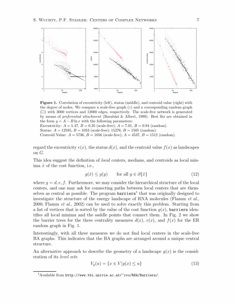
where g = d, e, f . Furthermore, we may consider the hierarchical structure of the localcenters, and one may ask for connecting paths between local centers that are them-selves as central as possible. The program barriers

1 that was originally designed toinvestigate the structure of the energy landscape of RNA molecules (Flamm et al.,2000; Flamm et al., 2002) can be used to solve exactly this problem. Starting froma list of vertices that is sorted by the value of the cost function g(x), barriers iden-tifies all local minima and the saddle points that connect them. In Fig. 2 we showthe barrier trees for the three centrality measures d(x), e(x), and f(x) for the ERrandom graph in Fig. 1.

Interestingly, with all three measures we do not find local centers in the scale-freeBA graphs. This indicates that the BA graphs are arranged around a unique centralstructure.

An alternative approach to describe the geometry of a landscape g(x) is the consid-eration of its level sets

Vg(u) = {x ∈ V |g(x) ≤ u} (13)

1Available from http://www.tbi.univie.ac.at/~ivo/RNA/Barriers/.


5.0

5.2

5.4

5.6

5.8

6.0

6.2

6.4

6.6

6.8

7.0

7.2

7.4

10800.0

11000.0

11200.0

11400.0

11600.0

11800.0

12000.0

0.0

200.0

400.0

600.0

800.0

1000.0

1200.0

e(x) d(x) f(x)

Figure 2. Barrier trees for excentricity (left), status (middle), and centroid value (right)for an ER random graph with 3000 vertices and 12000 nodes.

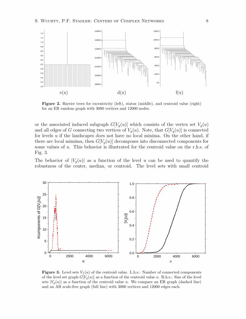
or the associated induced subgraph G[Vg(u)] which consists of the vertex set Vg(u)and all edges of G connecting two vertices of Vg(u). Note, that G[Vg(u)] is connectedfor levels u if the landscapes does not have no local minima. On the other hand, ifthere are local mimima, then G[Vg(u)] decomposes into disconnected components forsome values of u. This behavior is illustrated for the centroid value on the r.h.s. ofFig. 3.

The behavior of |Vg(u)| as a function of the level u can be used to quantify therobustness of the center, median, or centroid. The level sets with small centroid

0 2000 4000 6000

u

0

5

10

15

20

25

30

#com

pone

nts

of G

[Vf(u

)]

0 2000 4000 6000

u

0.0

0.2

0.4

0.6

0.8

1.0

|Vf(u

)|

Figure 3. Level sets Vf (u) of the centroid value. L.h.s.: Number of connected componentsof the level set graph G[Vg(u)] as a function of the centroid value u. R.h.s.: Size of the levelsets |Vg(u)| as a function of the centroid value u. We compare an ER graph (dashed line)and an AB scale-free graph (full line) with 3000 vertices and 12000 edges each.


values are smaller in the AB model indicating a tighter near central subgraph thanin the ER model. Not surprisingly, the ER model is more homogeneous on average.

4. Applications

4.1. Metabolic network. In metabolic networks, the meaning of centrality is ob-vious: The central metabolites are the crossroads of the networks and, in the spiritof the graph evolution models, also the historically oldest ones. Centrality thereforeshould reflect both age and importance. Local centers, if they exists, therefore arelikely the remnants of a previous merging, while the absence of local centers indicateda continuous, step-wise, growth the network.

(Fell & Wagner, 2000) assembled the central routes of the energy metabolism andsmall-molecule building block synthesis in E. coli and constructed a substrate graphwith the metabolites as vertices and edges connecting any two metabolites that ap-pear in the same reaction. In their analysis, ATP and H2O was excluded. (Jeonget al., 2000) considered metabolic networks of 43 different organisms including E.coli. Unlike (Fell & Wagner, 2000), a bipartite graph was used in which both thesubstrates and the reactions are vertices, and edges connect substrates with the re-actions they are taking part in. Both studies report a power-law degree distributioncharacteristic for scale-free networks.

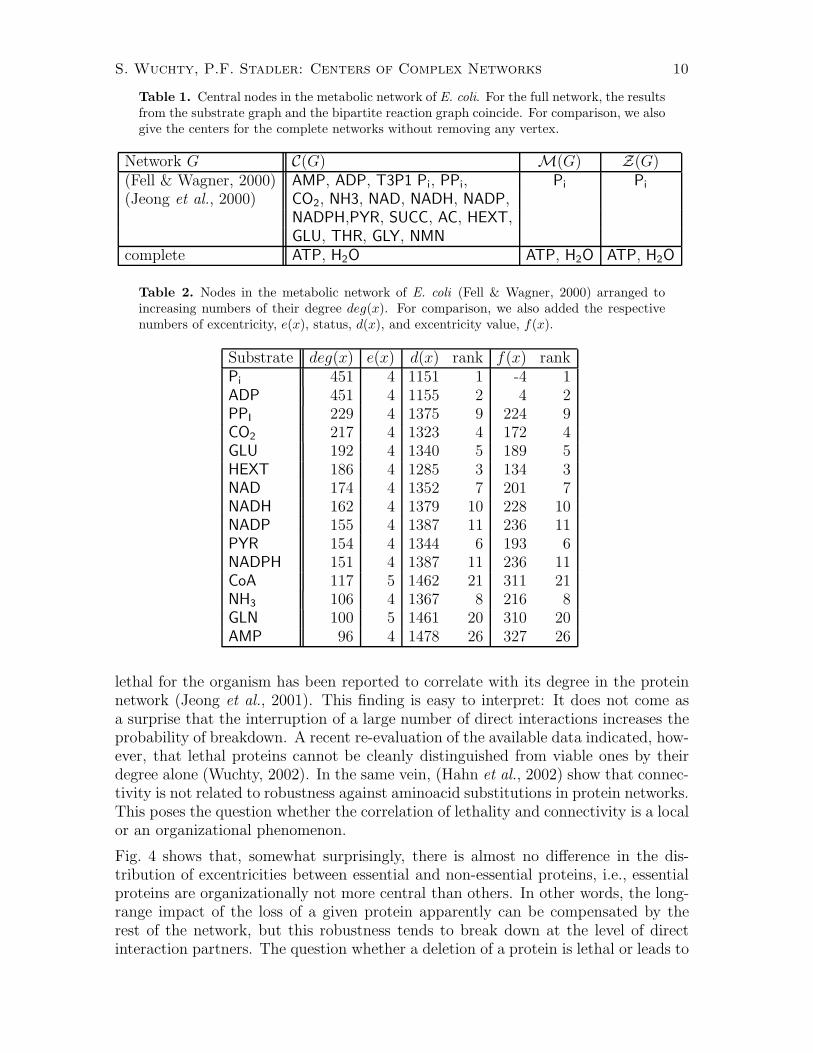
In Table 1, we list the center C(G), median C(G), and centroid Z(G). We find that theresults are identical for the substrate graph of (Fell & Wagner, 2000) and the bipartitereaction graph of (Jeong et al., 2000). Following the proceedure of (Fell & Wagner,2000), we deleted ATP and H2O from this graph because they are connected withalmost every other metabolite. Not surprisingly, we are left with inorganic phosphatePi and ADP at the next most connected vertices.

Interestingly, the most coarse grained measure, the center C(G) yields a good intuitiveestimate of the most centered substrates. Among these are ATP, ADP and AMP whichare obviously the most central substrates to the energetics and signaling pathwaysof the cell. In this regard, the frequent occurrence of Pi and PPi fits the pictureperfectly. Furthermore, NADP and NADPH appear in a similar context. Amongthe most popular metabolites, succinate SUCC, glutamate GLU, pyruvate PYR, andcoenzyme A COA appear in the center. These metabolites indeed play a “central”role in well known pathways emphasizing glycolysis and the citrate cycle.

A comparison of the nodes degree with their corresponding centrality measures showsthat a highly linked vertex has small numbers of the geometric centrality measures(see Table 2). It is striking that all three centrality measures e(x), d(x), and f(x)yield very similar rank orders close to the central vertices, despite the fact that thesemeasures may disagree significantly for non-central vertices, although the three no-tions of geometric centrality are conceptually quite different from each other. In fact,the rank of all metabolites listed in table 2 are the same for d(x) and f(x).

4.2. Protein Networks. A second class of networks that have received particularattention recently are networks of (direct) protein interaction (Jeong et al., 2001;Wagner, 2001). The likelihood that the elimination of a protein from the genome is


Table 1. Central nodes in the metabolic network of E. coli. For the full network, the resultsfrom the substrate graph and the bipartite reaction graph coincide. For comparison, we alsogive the centers for the complete networks without removing any vertex.

Network G C(G) M(G) Z(G)(Fell & Wagner, 2000) AMP, ADP, T3P1 Pi, PPi, Pi Pi

(Jeong et al., 2000) CO2, NH3, NAD, NADH, NADP,NADPH,PYR, SUCC, AC, HEXT,GLU, THR, GLY, NMN

complete ATP, H2O ATP, H2O ATP, H2O

Table 2. Nodes in the metabolic network of E. coli (Fell & Wagner, 2000) arranged toincreasing numbers of their degree deg(x). For comparison, we also added the respectivenumbers of excentricity, e(x), status, d(x), and excentricity value, f(x).

Substrate deg(x) e(x) d(x) rank f(x) rankPi 451 4 1151 1 -4 1ADP 451 4 1155 2 4 2PPI 229 4 1375 9 224 9CO2 217 4 1323 4 172 4GLU 192 4 1340 5 189 5HEXT 186 4 1285 3 134 3NAD 174 4 1352 7 201 7NADH 162 4 1379 10 228 10NADP 155 4 1387 11 236 11PYR 154 4 1344 6 193 6NADPH 151 4 1387 11 236 11CoA 117 5 1462 21 311 21NH3 106 4 1367 8 216 8GLN 100 5 1461 20 310 20AMP 96 4 1478 26 327 26

lethal for the organism has been reported to correlate with its degree in the proteinnetwork (Jeong et al., 2001). This finding is easy to interpret: It does not come asa surprise that the interruption of a large number of direct interactions increases theprobability of breakdown. A recent re-evaluation of the available data indicated, how-ever, that lethal proteins cannot be cleanly distinguished from viable ones by theirdegree alone (Wuchty, 2002). In the same vein, (Hahn et al., 2002) show that connec-tivity is not related to robustness against aminoacid substitutions in protein networks.This poses the question whether the correlation of lethality and connectivity is a localor an organizational phenomenon.

Fig. 4 shows that, somewhat surprisingly, there is almost no difference in the dis-tribution of excentricities between essential and non-essential proteins, i.e., essentialproteins are organizationally not more central than others. In other words, the long-range impact of the loss of a given protein apparently can be compensated by therest of the network, but this robustness tends to break down at the level of directinteraction partners. The question whether a deletion of a protein is lethal or leads to


0 5 10 15 20excentricity e(x)

0.00

0.05

0.10

0.15

0.20

0.25

0.30

0.35

freq

uenc

y

Figure 4. Frequency proteins with given excentricity values for ◦ all, N non-lethal, and H

lethal deletion mutants. There is no significant difference between the three datasets. Theprotein network graph is not connected, hence the distribution of the eccentricity, which wecompute as the superposition of the eccentricities of the individual components is bi-modal:One peak reflects the small components and the other, larger peak refers to the main (giant)component of the network.

a viable phenotype therefore will require a gradual answer. A promising approach inthis direction was recenly undertaken by (Jeong et al., 2002), who found correlationsof phenotypic effects of single gene deletions in Yeast with fluctuations in the corre-sponding mRNA expression levels, functional classification of gene products and thenumber of interactions in the underlying protein-protein interaction network. Basedon these qualitative measurements, they were able to predict gradual phenotypiceffects that are in good agreement with already known experimental results. The de-pendence of the degree of lethality on multiple factors, including the functional classof the protein, highlights the limitations of purely structural approaches to networkanalysis.

4.3. Domain Sequence Network. Many proteins consist of a number of recogniz-able domains that appear in oftentimes many different proteins. A graph G can beconstructed that has the domains as its vertices and edges between them whenevertwo domains co-occur in a protein. Essentially, they give a tentative insight intothe structure of the proteome since they were found to exhibit scale-free behavior.Thus, domains which prove to be highly connected since they frequently occur in mul-tidomain proteins shape the backbone of the proteome of the underlying organism.Similar to the metabolic networks, highly connected domains might have shaped anevolutionary core of proteomes.


0 1000 2000 3000 4000 5000 6000 7000centroid value u

0.0

0.2

0.4

0.6

0.8

1.0

|Vf(u

)|

E. coliS. cerevisiaeA. thalianaC. elegansD. melanogasterH. sapiens

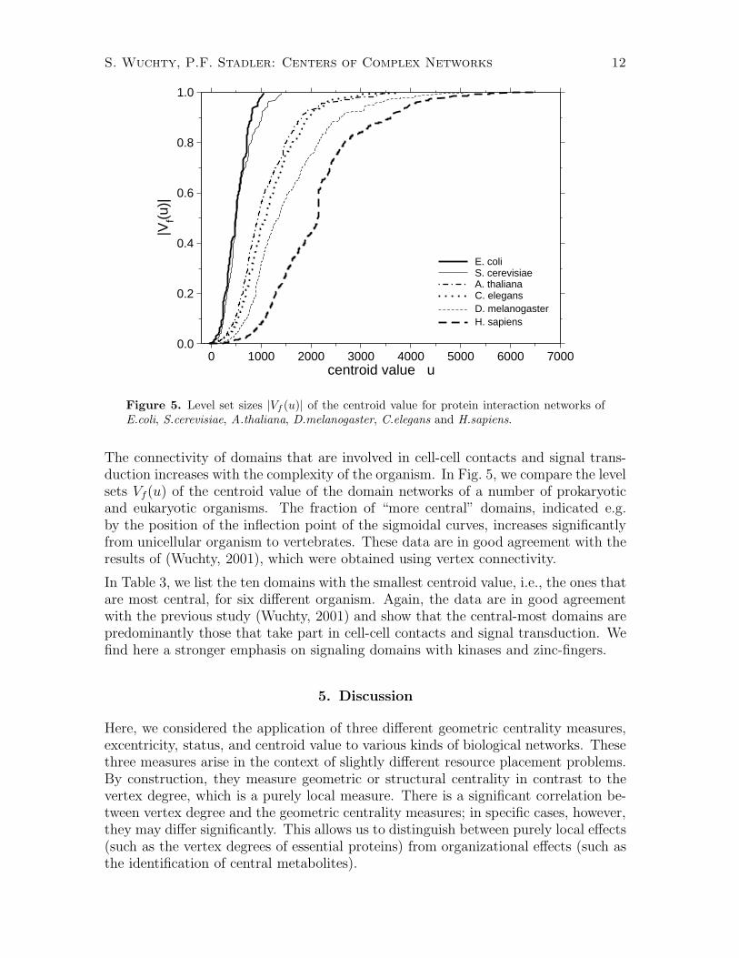
Figure 5. Level set sizes |Vf (u)| of the centroid value for protein interaction networks ofE.coli, S.cerevisiae, A.thaliana, D.melanogaster, C.elegans and H.sapiens.

The connectivity of domains that are involved in cell-cell contacts and signal trans-duction increases with the complexity of the organism. In Fig. 5, we compare the levelsets Vf(u) of the centroid value of the domain networks of a number of prokaryoticand eukaryotic organisms. The fraction of “more central” domains, indicated e.g.by the position of the inflection point of the sigmoidal curves, increases significantlyfrom unicellular organism to vertebrates. These data are in good agreement with theresults of (Wuchty, 2001), which were obtained using vertex connectivity.

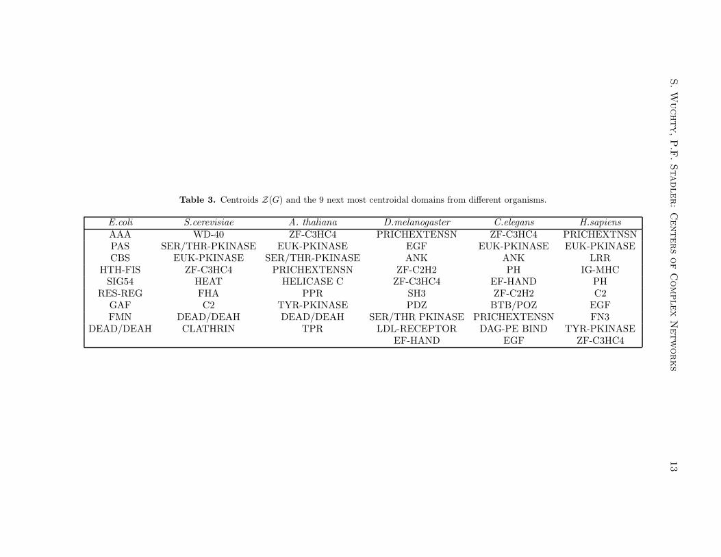
In Table 3, we list the ten domains with the smallest centroid value, i.e., the ones thatare most central, for six different organism. Again, the data are in good agreementwith the previous study (Wuchty, 2001) and show that the central-most domains arepredominantly those that take part in cell-cell contacts and signal transduction. Wefind here a stronger emphasis on signaling domains with kinases and zinc-fingers.

5. Discussion

Here, we considered the application of three different geometric centrality measures,excentricity, status, and centroid value to various kinds of biological networks. Thesethree measures arise in the context of slightly different resource placement problems.By construction, they measure geometric or structural centrality in contrast to thevertex degree, which is a purely local measure. There is a significant correlation be-tween vertex degree and the geometric centrality measures; in specific cases, however,they may differ significantly. This allows us to distinguish between purely local effects(such as the vertex degrees of essential proteins) from organizational effects (such asthe identification of central metabolites).

S.W

uchty,P.F

.Stadler:

Centers

of

Complex

Netw

orks

13

Table 3. Centroids Z(G) and the 9 next most centroidal domains from different organisms.

E.coli S.cerevisiae A. thaliana D.melanogaster C.elegans H.sapiens

AAA WD-40 ZF-C3HC4 PRICHEXTENSN ZF-C3HC4 PRICHEXTNSNPAS SER/THR-PKINASE EUK-PKINASE EGF EUK-PKINASE EUK-PKINASECBS EUK-PKINASE SER/THR-PKINASE ANK ANK LRR

HTH-FIS ZF-C3HC4 PRICHEXTENSN ZF-C2H2 PH IG-MHCSIG54 HEAT HELICASE C ZF-C3HC4 EF-HAND PH

RES-REG FHA PPR SH3 ZF-C2H2 C2GAF C2 TYR-PKINASE PDZ BTB/POZ EGFFMN DEAD/DEAH DEAD/DEAH SER/THR PKINASE PRICHEXTENSN FN3

DEAD/DEAH CLATHRIN TPR LDL-RECEPTOR DAG-PE BIND TYR-PKINASEEF-HAND EGF ZF-C3HC4


Since measures of centrality can be assigned to individual vertices of the networks,we can define not only global centers as the vertices that minimize (or maximize) acentrality measures, but we obtain as a natural definition of local centers in termsof local optima of the centrality value landscape on the network. In the connectedexamples that we have considered here, as well as the generic examples of scale-freenetworks, we did not encounter local centers; on the other hand, local centers areabundant in random networks.

Another important implication of local centers is that they are indicative of a modularorganization and possibly also of a modular origin of the network. If the network inquestion does not resemble a ER random graph, then local centers could be interpretedas the centers building blocks that were merged together. The absence of local centersis then a strong indication for the stepwise growth of the network.

Acknowledgments. We thank Hawoong Jeong for supplying his protein-proteininteraction data.

References

Albert, R. & Barabasi, A.-L. (2000a). Topology of evolving networks: local eventsand universality. Phys. Rev. Lett. , 5234–5237.

Albert, R. & Barabasi, A.-L. (2002). Statistical mechanics of complex networks. Rev.Mod. Phys. 74, 47–97.

Amaral, L. A. N., Scala, A., Barthelemy, M., & Stanley, H. E. (2000). Classes ofsmall world networks. Proc. Natl. Acad. Sci. USA, 97, 11149–11152.

Barabasi, A.-L. & Albert, R. (1999). Emergence of scaling in random networks.Science, 286, 509–512.

Barabasi, A.-L., Albert, R., & Jeong, H. (1999). Mean-field theory for scale-freerandom networks. Physica A, 173-187, 272.

Barefoot, C. A., Entringer, R. C., & Szekely, L. A. (1997). Extremal values for ratiosof distance trees. Discr. Appl. Math. 80, 37–56.

Barrat, A. & Weigt, M. (2000). On the properties of small-world network models.Europ. Phys. J. B, 13, 547–.

Berge, C. (1985). Graphs. Amsterdam, NL: North-Holland.Bollobas, B. (1985). Random Graphs. London UK: Academic Press.Cormen, T. H., Leiserson, C. E., & Rivest, R. L. (1990). Introduction to Algorithms.

Cambridge, MA: MIT Press.Entringer, R. C., Jackson, D. E., & Snyder, D. A. (1976). Distance in graphs.

Czechoslowak Math. J. 26, 283–296.Erdos, P. & Renyi, A. (1960). On the evolution of random graphs. Publ. Math. Inst.

Hung. Acad. Sci., Ser. A, 5, 17–61.Fell, D. A. & Wagner, A. (2000). The small world of metabolism. Nature Biotech.

189, 1121–1122.Flamm, C., Fontana, W., Hofacker, I. L., & Schuster, P. (2000). RNA folding at

elementary step resolution. RNA, 6, 325–338.Flamm, C., Hofacker, I. L., Stadler, P. F., & Wolfinger, M. T. (2002). Barrier trees

of degenerate landscape. Z. Phys. Chem. 216, 155–173.


Freeman, L. C. (1977). A set of measures of centrality based on betweenness. So-ciometry, 40, 35–41.

Gleiss, P. M., Stadler, P. F., Wagner, A., & Fell, D. A. (2001). Relevant cycles inchemical reaction network. Adv. Complex Syst. 4, 207–226.

Goh, K.-I., Oh, E. S., Jeong, H., Khang, B., & Kim, D. (2002). Classification ofscale-free networks. Technical Report 0205232 arXiv:cond-mat.

Gutman, I., Klavzar, S., & Mohar, B., eds (1996). Fifty Years of the Wiener indexvolume 36 of MATCH.

Hahn, M. W., Conant, G., & Wagner, A. (2002). Molecular evolution in large geneticnetworks: connectivity does not equal importance. Technical Report 02-08-039Santa Fe Institute.

Harary, F. (1959). Status and contrastatus. Sociometry, 22, 23–43.Harary, F. & Norman, R. Z. (1953). The dissimilarity characteristic of Husimi trees.

Ann. Math. 58, 134–141.Herzel, H. (1998). How to quantify “small world networks”? Fractals, 6, 301–303.Jeong, H., Mason, S. P., Barabasi, A.-L., & Oltvai, Z. N. (2001). Lethality and

centrality in protein networks. Nature, 411, 41–42.Jeong, H., Oltvai, Z. N., & Barabasi, A.-L. (2002). Prediction of protein essentiality

based on genomic data. in press, ComPlexUs.Jeong, H., Tombor, B., Albert, R., Oltvai, Z. N., & Barabasi, A.-L. (2000). The

large-scale organization of metabolic networks. Nature, 407, 651–654.Jordan, C. (1869). Sur les assemblages de lignes. J. Reine Angew. Math. 70, 185–190.Montoya, J. M. & Sole, R. V. (2002). Small world patterns in food webs. J. Theor.

Biol. . in press, Santa Fe Institute preprint 00-10-059.Newman, M. E. J., Moore, C., & Watts, D. J. (2000). Mean-field solution of the

small-world network model. Phys. Rev. Lett. 84, 3201–3204.Newman, M. E. J. & Watts, D. J. (1999). Renormalization group analysis of the

small-world network model. Phys. Lett. A, 263, 341–346.Nieminen, J. (1984). Centrality, convexity and intersections in graphs. Bull. Math.

Soc. Sci. Math. Repub. Soc. Roum., Nouv. Ser, 28(76), 337–344.Reidys, C. M. & Stadler, P. F. (2002). Combinatorial landscapes. SIAM Review, 44,

3–54.Slater, P. J. (1975). Maximum facility location. J. Res. Natl. Bur Stand. B, 79,

107–115.Slater, P. J. (1976). Central vertices in a graph. Congr. Num. 17, 487–487. Proc.

7th Southeast. Conf. Comb., Graph Theory, Comput.; Baton Rouge.Slater, P. J. (1980). Medians of arbitrary graphs. J. Graph Theory, 4, 389–392.Slater, P. J. (1999). A survey of sequences of central subgraphs. Networks, 34,

224–249.Smart, C. & Slater, P. J. (1999). Center, median, and centroid subgraphs. Networks,

34, 303–311.Wagner, A. (2001). The yeast protein interaction network evolves rapidly and contains

few redundant duplicate genes. Mol. Biol. Evol. 18, 1283–1292.Wagner, A. & Fell, D. A. (2000). The small world inside large metabolic networks.

Technical Report 00-07-041 Santa Fe Institute.Watts, D. J. (1999). Small Worlds. Princeton NJ: Princeton University Press.


Watts, D. J. & Strogatz, H. S. (1998). Collective dynamics of “small-world” networks.Nature, 393, 440–442.

Wiener, H. (1947). Structural determination of paraffine boiling points. J. Amer.Chem. Soc. 69, 17–20.

Wright, S. (1932). The roles of mutation, inbreeding, crossbreeeding and selectionin evolution. In: Proceedings of the Sixth International Congress on Genetics,(Jones, D. F., ed) volume 1 pp. 356–366, New York: Brooklyn Botanic Gardens.

Wright, S. (1967). “surfaces” of selective value. Proc. Nat. Acad. Sci. USA, 58,165–172.

Wuchty, S. (2001). Scale-free behavior in protein domain networks. Mol. Biol. Evol.18, 1694–1702.

Wuchty, S. (2002). Interaction and domain networks of yeast. Proteomics, . in press.Zelinka, B. (1968). Medians and peripherans of trees. Arch. Math. (Brno), 4, 87–95.

centers of complex networks - bioinf.uni-leipzig.de

Documents