control of nonlinear active vehicle suspension systems using

0

Control of Nonlinear Active Vehicle SuspensionSystems Using Disturbance Observers

Francisco Beltran-Carbajal1, Esteban Chavez-Conde2,

Gerardo Silva Navarro3, Benjamin Vazquez Gonzalez1

and Antonio Favela Contreras4

1Universidad Autonoma Metropolitana, Plantel Azcapotzalco,Departamento de Energia, Mexico, D.F.

2Universidad del Papaloapan, Campus Loma Bonita, Departamento de Ingenieria en

Mecatronica, Instituto de Agroingenieria, Loma Bonita, Oaxaca3Centro de Investigacion y de Estudios Avanzados del I.P.N., Departamento de Ingenieria

Electrica, Seccion de Mecatronica, Mexico, D.F.4ITESM Campus Monterrey, Monterrey, N.L.

Mexico

1. Introduction

The main control objectives of active vehicle suspension systems are to improve the ride

comfort and handling performance of the vehicle by adding degrees of freedom to the

passive system and/or controlling actuator forces depending on feedback and feedforward

information of the system obtained from sensors.

Passenger comfort is provided by isolating the passengers from the undesirable vibrations

induced by irregular road disturbances and its performance is evaluated by the level of

acceleration by which vehicle passengers are exposed. Handling performance is achieved

by maintaining a good contact between the tire and the road to provide guidance along the

track.

The topic of active vehicle suspension control system, for linear and nonlinear models, in

general, has been quite challenging over the years and we refer the reader to some of the

fundamental works in the vibration control area (Ahmadian, 2001). Some active control

schemes are based on neural networks, genetic algorithms, fuzzy logic, sliding modes,

H-infinity, adaptive control, disturbance observers, LQR, backstepping control techniques,

etc. See, e.g., (Cao et al., 2008); (Isermann & Munchhof, 2011); (Martins et al., 2006); (Tahboub,

2005); (Chen & Huang, 2005) and references therein. In addition, some interesting semiactive

vibration control schemes, based on Electro-Rheological (ER) and Magneto-Rheological (MR)

dampers, have been proposed and implemented on commercial vehicles. See, e.g., (Choi et al.,

2003); (Yao et al., 2002).

In this chapter is proposed a robust control scheme, based on the real-time estimation of

perturbation signals, for active nonlinear or linear vehicle suspension systems subject to

unknown exogenous disturbances due to irregular road surfaces. Our approach differs

7

www.intechopen.com

2 Vibration Control

from others in that, the control design problem is formulated as a bounded disturbance

signal processing problem, which is quite interesting because one can take advantage of the

industrial embedded system technologies to implement the resulting active vibration control

strategies. In fact, there exist successful implementations of automotive active control systems

based on embedded systems, and this novel tendency is growing very fast in the automotive

industry. See, e.g., (Shoukry et al., 2010); (Basterretxea et al., 2010); (Ventura et al., 2008);

(Gysen et al., 2008) and references therein.

In our control design approach is assumed that the nonlinear effects, parameter variations,

exogenous disturbances and possibly input unmodeled dynamics are lumped into an

unknown bounded time-varying disturbance input signal affecting a so-called differentially

flat linear simplified dynamic mathematical model of the suspension system. The lumped

disturbance signal and some time derivatives of the flat output are estimated by using a

flat output-based linear high-gain dynamic observer. The proposed observer-control design

methodology considers that, the perturbation signal can be locally approximated by a family

of Taylor polynomials. Two active vibration controllers are proposed for hydraulic or

electromagnetic suspension systems, which only require position measurements.

Some numerical simulation results are provided to show the efficiency, effectiveness and

robust performance of the feedforward and feedback linearization control scheme proposed

for a nonlinear quarter-vehicle active suspension system.

This chapter is organized as follows: Section 2 presents the nonlinear mathematical model

of an active nonlinear quarter-vehicle suspension system. Section 3 presents the proposed

vehicle suspension control scheme based on differential flatness. Section 4 presents the

main results of this chapter as an alternative solution to the vibration attenuation problem

in nonlinear and linear active vehicle suspension systems actuated electromagnetically or

hydraulically. Computer simulation results of the proposed design methodology are included

in Section 5. Finally, Section 6 contains the conclusions and suggestions for further research.

2. A quarter-vehicle active suspension system model

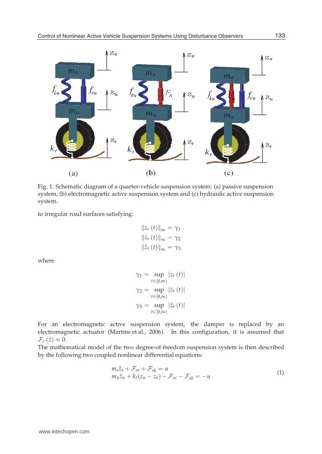
Consider the well-known nonlinear quarter-vehicle suspension system shown in Fig. 1. In

this model, the sprung mass ms denotes the time-varying mass of the vehicle-body and the

unsprung mass mu represents the assembly of the axle and wheel. The tire is modeled as a

linear spring with equivalent stiffness coefficient kt linked to the road and negligible damping

coefficient. The vehicle suspension, located between ms and mu, is modeled by a damper and

spring, whose nonlinear damping and stiffness force functions are given by

Fk (z) = kz + knz3

Fc (z) = cz + cn z2sgn(z)

The generalized coordinates are the displacements of both masses, zs and zu, respectively. In

addition, u = FA denotes the (force) control input, which is applied between the two masses

by means of an actuator, and zr (t) represents a bounded exogenous perturbation signal due

132 Vibration Analysis and Control – New Trends and Development

www.intechopen.com

Control of Nonlinear Active Vehicle Suspension Systems Using Disturbance Observers 3

Fig. 1. Schematic diagram of a quarter-vehicle suspension system: (a) passive suspensionsystem, (b) electromagnetic active suspension system and (c) hydraulic active suspensionsystem.

to irregular road surfaces satisfying:

‖zr (t)‖∞ = γ1

‖zr (t)‖∞ = γ2

‖zr (t)‖∞ = γ3

where

γ1 = supt∈[0,∞)

|zr (t)|

γ2 = supt∈[0,∞)

|zr (t)|

γ3 = supt∈[0,∞)

|zr (t)|

For an electromagnetic active suspension system, the damper is replaced by an

electromagnetic actuator (Martins et al., 2006). In this configuration, it is assumed that

Fc (z) ≈ 0.

The mathematical model of the two degree-of-freedom suspension system is then described

by the following two coupled nonlinear differential equations:

ms zs +Fsc +Fsk = u

mu zu + kt(zu − zr)−Fsc −Fsk = −u(1)

133Control of Nonlinear Active Vehicle Suspension Systems Using Disturbance Observers

www.intechopen.com

4 Vibration Control

withFsk (zs, zu) = ks(zs − zu) + kns (zs − zu)

3

Fsc (zs, zu) = cs(zs − zu) + cns(zs − zu)2sgn(zs − zu)

where sgn(·) denotes the standard signum function.

Defining the state variables as x1 = zs, x2 = zs, x3 = zu and x4 = zu, one obtains the following

state-space description:

x1 = x2

x2 = − 1ms

(Fsc +Fsk) +1

msu

x3 = x4

x4 = − ktmu

x3 +1

mu(Fsc +Fsk)−

1mu

u + ktmu

zr

(2)

withFsk (x1, x3) = ks(x1 − x3) + kns (x1 − x3)

3

Fsc (x2, x4) = cs(x2 − x4) + cns(x2 − x4)2sgn(x2 − x4)

It is easy to verify that the nonlinear vehicle suspension system (2) is completely controllable

and observable and, therefore, is differentially flat and constructible. For more details

on this topics we refer to (Fliess et al., 1993) and the book by (Sira-Ramirez & Agrawal,

2004). Both properties can be used extensively during the synthesis of different controllers

based on differential flatness, trajectory planning, disturbance and state reconstruction,

parameter identification, Generalized PI (GPI) and sliding mode control, etc. See, e.g.,

(Beltran-Carbajal et al., 2010a); (Beltran-Carbajal et al., 2010b); (Chavez-Conde et al., 2009a);

(Chavez-Conde et al., 2009b).

In what follows, a feedforward and feedback linearization active vibration controller, as

well as a disturbance observer, will be designed taking advantage of the differential flatness

property exhibited by the vehicle suspension system.

3. Differential flatness-based control

The system (2) is differentially flat, with a flat output given by

L = msx1 + mux3

which is constructed as a linear combination of the displacements of the sprung mass x1 and

the unsprung mass x3.

Then, all the state variables and the control input can be parameterized in terms of the flat

output L and a finite number of its time derivatives (Sira-Ramirez & Agrawal, 2004). As a

matter of fact, from L and its time derivatives up to fourth order one can obtain:

L = msx1 + mux3

L = msx2 + mux4

L = kt (zr − x3)

L(3) = kt (zr − x4)

L(4) = 1mu

u + ktmu

x3 −1

mu(Fsc +Fsk)−

ktmu

zr + kt zr

(3)


www.intechopen.com


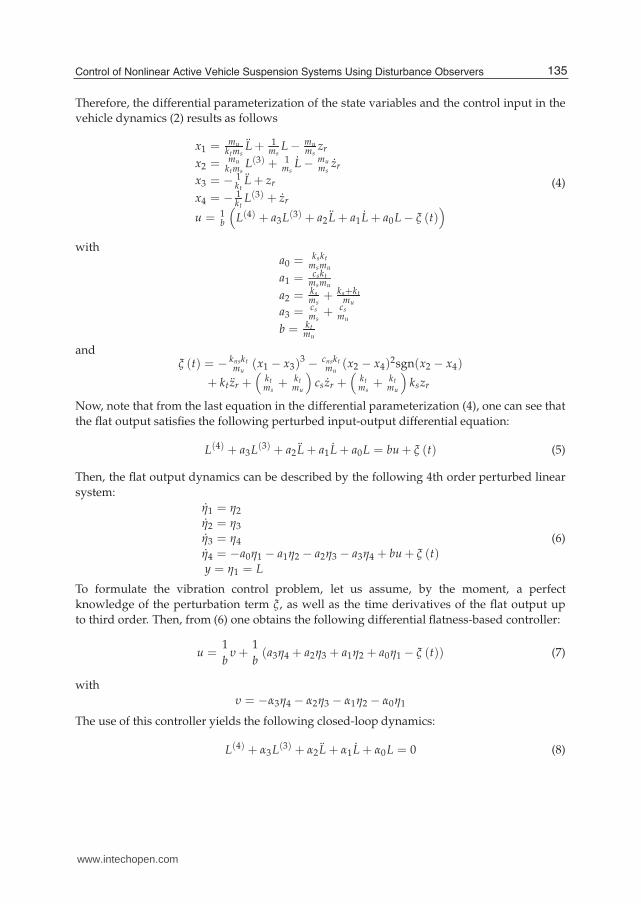
Therefore, the differential parameterization of the state variables and the control input in the

vehicle dynamics (2) results as follows

x1 = muktms

L + 1ms

L − mums

zr

x2 = muktms

L(3) + 1ms

L − mums

zr

x3 = − 1kt

L + zr

x4 = − 1kt

L(3) + zr

u = 1b

(L(4) + a3L(3) + a2 L + a1 L + a0L − ξ (t)

)(4)

witha0 = kskt

msmu

a1 = csktmsmu

a2 = ksms

+ ks+ktmu

a3 = csms

+ csmu

b = ktmu

andξ (t) = − knskt

mu(x1 − x3)

3 − cnsktmu

(x2 − x4)2sgn(x2 − x4)

+ kt zr +(

ktms

+ ktmu

)cs zr +

(ktms

+ ktmu

)kszr

Now, note that from the last equation in the differential parameterization (4), one can see that

the flat output satisfies the following perturbed input-output differential equation:

L(4) + a3L(3) + a2 L + a1 L + a0L = bu + ξ (t) (5)

Then, the flat output dynamics can be described by the following 4th order perturbed linear

system:

η1 = η2

η2 = η3

η3 = η4

η4 = −a0η1 − a1η2 − a2η3 − a3η4 + bu + ξ (t)y = η1 = L

(6)

To formulate the vibration control problem, let us assume, by the moment, a perfect

knowledge of the perturbation term ξ, as well as the time derivatives of the flat output up

to third order. Then, from (6) one obtains the following differential flatness-based controller:

u =1

bυ +

1

b(a3η4 + a2η3 + a1η2 + a0η1 − ξ (t)) (7)

with

υ = −α3η4 − α2η3 − α1η2 − α0η1

The use of this controller yields the following closed-loop dynamics:

L(4) + α3L(3) + α2 L + α1 L + α0L = 0 (8)


www.intechopen.com

6 Vibration Control

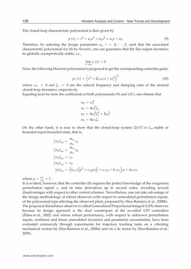
The closed-loop characteristic polynomial is then given by

p (s) = s4 + α3s3 + α2s2 + α1s + α0 (9)

Therefore, by selecting the design parameters αi, i = 0, · · · , 3, such that the associated

characteristic polynomial for (8) be Hurwitz, one can guarantee that the flat output dynamics

be globally asymptotically stable, i.e.,

limt→∞

L (t) = 0

Now, the following Hurwitz polynomial is proposed to get the corresponding controller gains:

pc (s) =(

s2 + 2ζcωcs + ω2c

)2(10)

where ωc > 0 and ζc > 0 are the natural frequency and damping ratio of the desired

closed-loop dynamics, respectively.

Equating term by term the coefficients of both polynomials (9) and (10 ), one obtains that

α0 = ω4c

α1 = 4ω3c ζc

α2 = 4ω2c ζ2

c + 2ω2c

α3 = 4ωcζc

On the other hand, it is easy to show that the closed-loop system (2)-(7) is L∞-stable or

bounded-input-bounded-state, that is,

‖x1‖∞ =mu

msγ1

‖x2‖∞ =mu

msγ2

‖x3‖∞ = γ1

‖x4‖∞ = γ2

‖u‖∞ =(

knsγ31ρ2 + cnsργ2

2 + csγ2 + ksγ1

)ρ + muγ3

where ρ = mums

+ 1.

It is evident, however, that the controller (8) requires the perfect knowledge of the exogenous

perturbation signal zr and its time derivatives up to second order, revealing several

disadvantages with respect to other control schemes. Nevertheless, one can take advantage of

the design methodology of robust observers with respect to unmodeled perturbation inputs,

of the polynomial type affecting the observed plant, proposed by (Sira-Ramirez et al., 2008b).

The proposed disturbance observer is called Generalized Proportional Integral (GPI) observer,

because its design approach is the dual counterpart of the so-called GPI controllers

(Fliess et al., 2002) and whose robust performance, with respect to unknown perturbation

inputs, nonlinear and linear unmodeled dynamics and parametric uncertainties, have been

evaluated extensively through experiments for trajectory tracking tasks on a vibrating

mechanical system by (Sira-Ramirez et al., 2008a) and on a dc motor by (Sira-Ramirez et al.,

2009).


www.intechopen.com


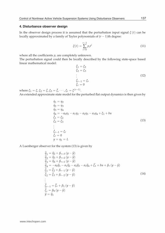
4. Disturbance observer design

In the observer design process it is assumed that the perturbation input signal ξ (t) can be

locally approximated by a family of Taylor polynomials of (r − 1)th degree:

ξ(t) =r−1

∑i=0

piti (11)

where all the coefficients pi are completely unknown.

The perturbation signal could then be locally described by the following state-space based

linear mathematical model:ξ1 = ξ2

ξ2 = ξ3

...

ξr−1 = ξr

ξr = 0

(12)

where ξ1 = ξ, ξ2 = ξ, ξ3 = ξ, · · · , ξr = ξ(r−1).

An extended approximate state model for the perturbed flat output dynamics is then given by

η1 = η2

η2 = η3

η3 = η4

η4 = −a0η1 − a1η2 − a2η3 − a3η4 + ξ1 + bu

ξ1 = ξ2

ξ2 = ξ3...

ξr−1 = ξr

ξr = 0

y = η1 = L

(13)

A Luenberger observer for the system (13) is given by

η1 = η2 + βr+3 (y − y)η2 = η3 + βr+2 (y − y)η3 = η4 + βr+1 (y − y)η4 = −a0η1 − a1η2 − a2η3 − a3 η4 + ξ1 + bu + βr (y − y)ξ1 = ξ2 + βr−1 (y − y)ξ2 = ξ3 + βr−2 (y − y)...ξr−1 = ξr + β1 (y − y)ξr = β0 (y − y)y = η1

(14)


www.intechopen.com

8 Vibration Control

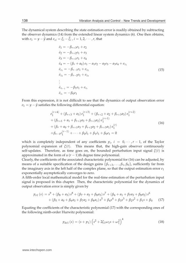
The dynamical system describing the state estimation error is readily obtained by subtracting

the observer dynamics (14) from the extended linear system dynamics (6). One then obtains,

with e1 = y − y and ezi = ξi − ξi , i = 1, 2, · · · , r, that

e1 = −βr+3e1 + e2

e2 = −βr+2e1 + e3

e3 = −βr+1e1 + e4

e4 = − (βr + a0) e1 − a1e2 − a2e3 − a3e4 + ez1

ez1 = −βr−1e1 + ez2

ez2 = −βr−2e1 + ez3

...

ezr−1 = −β1e1 + ezr

ezr = −β0e1

(15)

From this expression, it is not difficult to see that the dynamics of output observation error

e1 = y − y satisfies the following differential equation:

e(r+4)1 + (βr+3 + a3) e

(r+3)1 + (βr+2 + a2 + βr+3a3) e

(r+2)1

+ (βr+1 + a1 + βr+2a3 + βr+3a2) e(r+1)1

+ (βr + a0 + βr+1a3 + βr+2a2 + βr+3a1) e(r)1

+βr−1e(r−1)1 + · · ·+ β2 e1 + β1 e1 + β0e1 = 0

(16)

which is completely independent of any coefficients pi, i = 0, · · · , r − 1, of the Taylor

polynomial expansion of ξ(t). This means that, the high-gain observer continuously

self-updates. Therefore, as time goes on, the bounded perturbation input signal ξ(t) is

approximated in the form of a (r − 1)th degree time polynomial.

Clearly, the coefficients of the associated characteristic polynomial for (16) can be adjusted, by

means of a suitable specification of the design gains {βr+3, . . . , β1, β0}, sufficiently far from

the imaginary axis in the left half of the complex plane, so that the output estimation error e1

exponentially asymptotically converges to zero.

A fifth-order local mathematical model for the real-time estimation of the perturbation input

signal is proposed in this chapter. Then, the characteristic polynomial for the dynamics of

output observation error is simply given by

po1 (s) = s9 + (β8 + a3) s8 + (β7 + a2 + β8a3) s7 + (β6 + a1 + β7a3 + β8a2) s6

+ (β5 + a0 + β6a3 + β7a2 + β8a1) s5 + β4s4 + β3s3 + β2s2 + β1s + β0 (17)

Equating the coefficients of the characteristic polynomial (17) with the corresponding ones of

the following ninth-order Hurwitz polynomial:

pdo1 (s) = (s + p1)(

s2 + 2ζ1ω1s + ω21

)4(18)


www.intechopen.com


one gets the observer gains as follows

β0 = p1ω81

β1 = ω81 + 8p1ζ1ω7

1

β2 = 8ω71ζ1 + 24p1ω6

1ζ21 + 4p1ω6

1

β3 = 24ω61ζ2

1 + 4ω61 + 32p1ω5

1ζ31 + 24p1ω5

1ζ1

β4 = 32ω51ζ3

1 + 24ω51ζ1 + 16p1ω4

1ζ41 + 48p1ω4

1ζ21 + 6p1ω4

1

β5 = 16ω41ζ4

1 + 48ω41ζ2

1 + 6ω41 + 32p1ω3

1ζ31 + 24p1ω3

1ζ1 − a0 − β6a3 − β7a2 − β8a1

β6 = 32ω31ζ3

1 + 24ω31ζ1 + 24p1ω2

1ζ21 + 4p1ω2

1 − a1 − β7a3 − β8a2

β7 = 24ω21ζ2

1 + 4ω21 + 8p1ω1ζ1 − a2 − β8a3

β8 = p1 + 8ω1ζ1 − a3

with p1, ω1, ζ1 > 0.

Now, consider that the system (6) is being perturbed by the unknown input signal (t) as

followsη1 = η2

η2 = η3

η3 = η4

η4 = bu + (t)

y = η1 = L

(19)

with

(t) = −a0η1 − a1η2 − a2η3 − a3η4 + ξ (t)

Then, by the perfect knowledge of (t), one gets the following differential flatness-based

controller with feedforward of the perturbation signal (t):

u =1

b(υ − (t)) (20)

with

υ = −α3η4 − α2η3 − α1η2 − α0η1

Similarly as before, the perturbation input signal could be locally reconstructed by the

following family of Taylor polynomial of (r − 1)th degree:

(t) =r−1

∑i=0

γiti (21)

where all the coefficients γi are completely unknown.

Then, one can use the following extended mathematical model described in state-space

form to design a robust observer for real-time estimation of the disturbance (t) and time


www.intechopen.com

10 Vibration Control

derivatives of the flat output required for implementation of the controller (20):

η1 = η2

η2 = η3

η3 = η4

η4 = 1 + bu˙ 1 = 2

˙ 2 = 3...

˙ r−1 = r

˙ r = 0

y = η1 = L

(22)

where 1 = , 2 = ˙ , 3 = ¨ , · · · , r = (r−1).

A Luenberger observer for the system (22) is then given by

η1 = η2 + λr+3 (y − y)η2 = η3 + λr+2 (y − y)η3 = η4 + λr+1 (y − y)η4 = 1 + bu + λr (y − y)

1 = 2 + λr−1 (y − y)

2 = 3 + λr−2 (y − y)...

r−1 = r + λ1 (y − y) r = λ0 (y − y)y = η1

(23)

The estimation error dynamics e1 = y − y satisfies the following dynamics:

e(r+4)1 + λr+3e

(r+3)1 + λr+2e

(r+2)1 + λr+1e

(r+1)1 + λre

(r)1

+λr−1e(r−1)1 + · · ·+ λ2 e + λ1 e1 + λ0e1 = 0

(24)

Therefore, the design parameters λi, i = 0, · · · , r + 3, can be chosen so that the output

estimation error e1 exponentially asymptotically converges to zero.

On the other hand, it is assumed that the perturbation input signal (t) can be locally

approximated by a family of Taylor polynomials of fourth degree. Therefore, the characteristic

polynomial for the dynamics of output observation error (24) is given by

po2 = s9 + λ8s8 + λ7s7 + λ6s6 + λ5s5 + λ4s4 + λ3s3 + λ2s2 + λ1s + λ0 (25)

It is then proposed the following Hurwitz polynomial to compute the proper gains for the

observer:

po2 (s) = (s + p2)(

s2 + 2ζ2ω2s + ω22

)4(26)


www.intechopen.com


One then obtains that

λ0 = p2ω82

λ1 = ω82 + 8p2ζ2ω7

2

λ2 = 8ω72ζ2 + 24p2ω6

2ζ22 + 4p2ω6

2

λ3 = 24ω62ζ2

2 + 4ω62 + 32p2ω5

2ζ32 + 24p2ω5

2ζ2

λ4 = 32ω52ζ3

2 + 24ω52ζ2 + 16p2ω4

2ζ42 + 48p2ω4

2ζ22 + 6p2ω4

2

λ5 = 16ω42ζ4

2 + 48ω42ζ2

2 + 6ω42 + 32p2ω3

2ζ32 + 24p2ω3

2ζ2

λ6 = 32ω32ζ3

2 + 24ω32ζ2 + 24p2ω2

2ζ22 + 4p2ω2

2

λ7 = 24ω22ζ2

2 + 4ω22 + 8p2ω2ζ2

λ8 = p2 + 8ω2ζ2

with p2, ω2, ζ2 > 0.

From the practical viewpoint, main advantage of this high-gain observer is that it could be

employed for hydraulic or electromagnetic active vehicle suspension systems, requiring only

information of the stiffness constant of tire kt and the unsprung mass mu. In addition, it

can be shown that the proposed observer design methodology is quite robust with respect to

parameter uncertainty and unmodeled dynamics, by considering the parameter variations

into the perturbation input signal (t). In fact, in (Sira-Ramirez et al., 2008a) has been

presented through some experimental results that the polynomial disturbance signal-based

GPI control scheme, implemented as a classical compensation network, is robust enough with

respect to parameter uncertainty and unmodeled dynamics in the context of an off-line and

pre-specified reference trajectory tracking tasks.

It is important to emphasize that, the proposed results are now possible thanks to the existence

of commercial embedded system for automatic control tasks based on high speed FPGA/DSP

boards with high computational performance operating at high sampling rates. The proposed

observer could be implemented via embedded software applications without many problems.

5. Simulation results

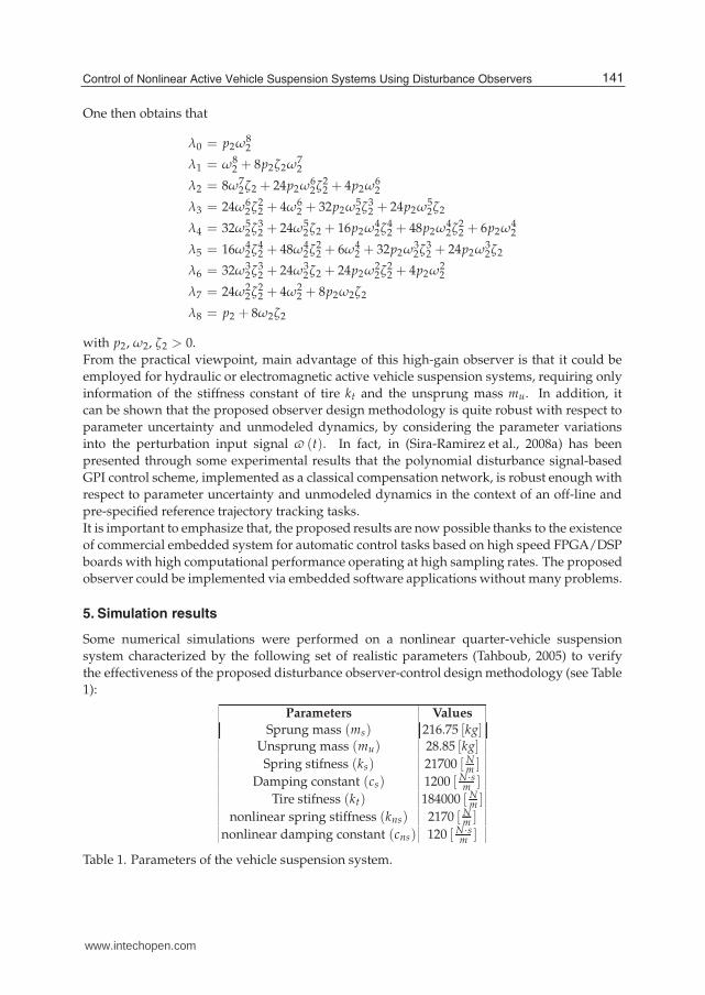
Some numerical simulations were performed on a nonlinear quarter-vehicle suspension

system characterized by the following set of realistic parameters (Tahboub, 2005) to verify

the effectiveness of the proposed disturbance observer-control design methodology (see Table

1):

Parameters Values

Sprung mass (ms) 216.75 [kg]Unsprung mass (mu) 28.85 [kg]

Spring stifness (ks) 21700 [ Nm ]

Damping constant (cs) 1200 [ N·sm ]

Tire stifness (kt) 184000 [ Nm ]

nonlinear spring stiffness (kns) 2170 [ Nm ]

nonlinear damping constant (cns) 120 [ N·sm ]

Table 1. Parameters of the vehicle suspension system.


www.intechopen.com


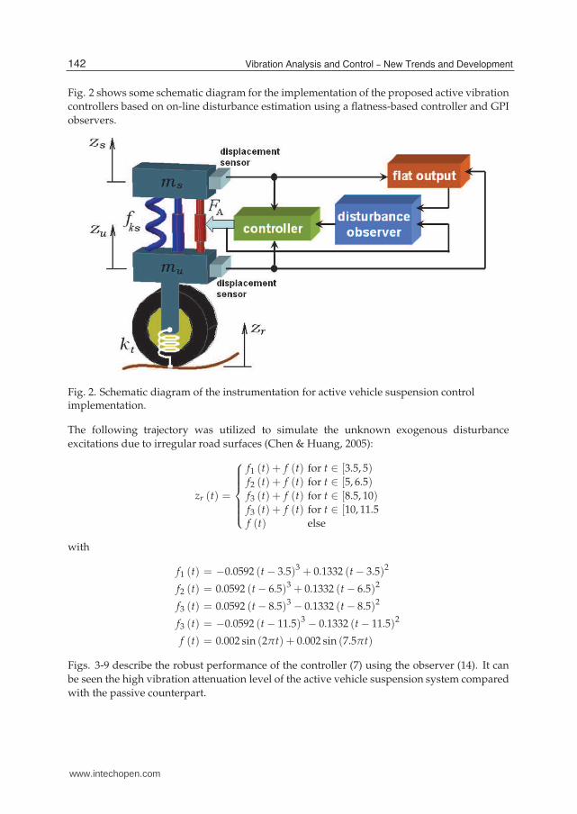
Fig. 2 shows some schematic diagram for the implementation of the proposed active vibration

controllers based on on-line disturbance estimation using a flatness-based controller and GPI

observers.

Fig. 2. Schematic diagram of the instrumentation for active vehicle suspension controlimplementation.

The following trajectory was utilized to simulate the unknown exogenous disturbance

excitations due to irregular road surfaces (Chen & Huang, 2005):

zr (t) =

⎧⎪⎪⎪⎪⎨⎪⎪⎪⎪⎩

f1 (t) + f (t) for t ∈ [3.5, 5)f2 (t) + f (t) for t ∈ [5, 6.5)f3 (t) + f (t) for t ∈ [8.5, 10)f3 (t) + f (t) for t ∈ [10, 11.5

f (t) else

with

f1 (t) = −0.0592 (t − 3.5)3 + 0.1332 (t − 3.5)2

f2 (t) = 0.0592 (t − 6.5)3 + 0.1332 (t − 6.5)2

f3 (t) = 0.0592 (t − 8.5)3 − 0.1332 (t − 8.5)2

f3 (t) = −0.0592 (t − 11.5)3 − 0.1332 (t − 11.5)2

f (t) = 0.002 sin (2πt) + 0.002 sin (7.5πt)

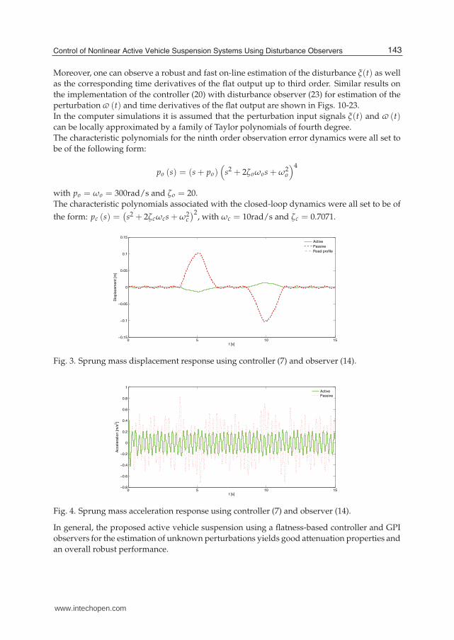
Figs. 3-9 describe the robust performance of the controller (7) using the observer (14). It can

be seen the high vibration attenuation level of the active vehicle suspension system compared

with the passive counterpart.


www.intechopen.com


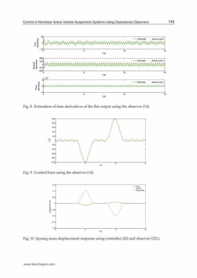
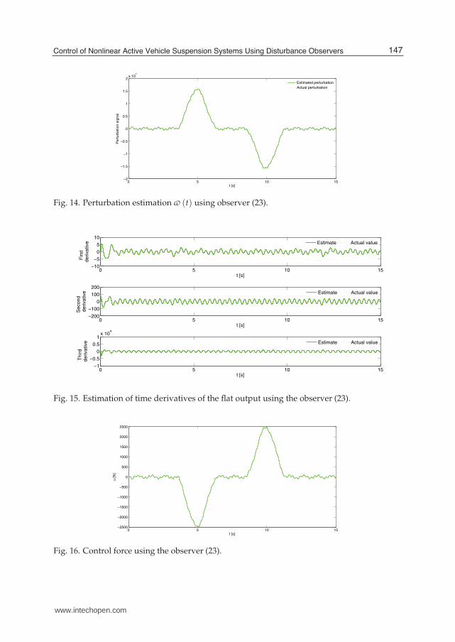
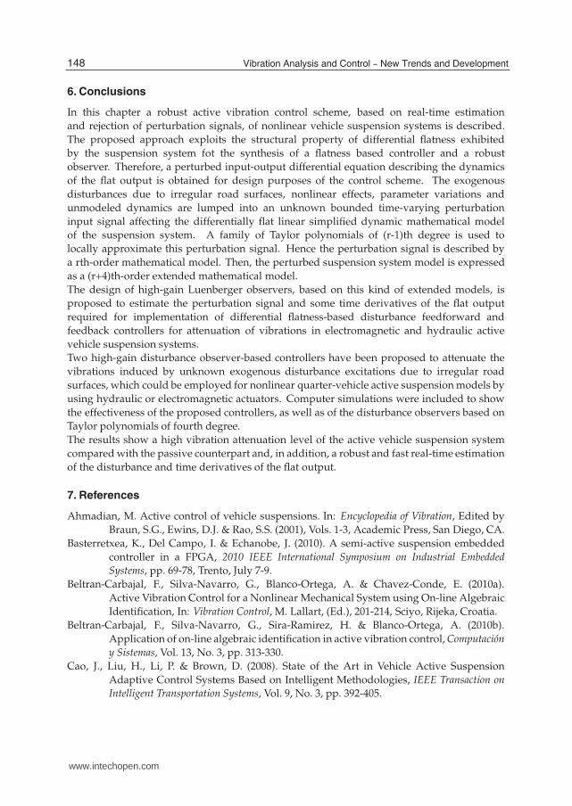
Moreover, one can observe a robust and fast on-line estimation of the disturbance ξ(t) as well

as the corresponding time derivatives of the flat output up to third order. Similar results on

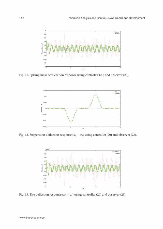
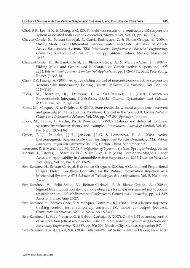
the implementation of the controller (20) with disturbance observer (23) for estimation of the

perturbation (t) and time derivatives of the flat output are shown in Figs. 10-23.

In the computer simulations it is assumed that the perturbation input signals ξ(t) and (t)can be locally approximated by a family of Taylor polynomials of fourth degree.

The characteristic polynomials for the ninth order observation error dynamics were all set to

be of the following form:

po (s) = (s + po)(

s2 + 2ζoωos + ω2o

)4

with po = ωo = 300rad/s and ζo = 20.

The characteristic polynomials associated with the closed-loop dynamics were all set to be of

the form: pc (s) =(s2 + 2ζcωcs + ω2

c

)2, with ωc = 10rad/s and ζc = 0.7071.

0 5 10 15−0.15

−0.1

−0.05

0

0.05

0.1

0.15

t [s]

Dis

pla

ce

me

nt

[m]

Active

Passive

Road profile

Fig. 3. Sprung mass displacement response using controller (7) and observer (14).

0 5 10 15−0.8

−0.6

−0.4

−0.2

0

0.2

0.4

0.6

0.8

1

t [s]

Acce

lera

tio

n [

m/s

2]

Active

Passive

Fig. 4. Sprung mass acceleration response using controller (7) and observer (14).

In general, the proposed active vehicle suspension using a flatness-based controller and GPI

observers for the estimation of unknown perturbations yields good attenuation properties and

an overall robust performance.


www.intechopen.com


0 5 10 15−0.15

−0.1

−0.05

0

0.05

0.1

0.15

t [s]

De

fle

ctio

n [

m]

Active

Passive

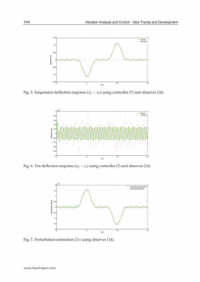
Fig. 5. Suspension deflection response (x1 − x3) using controller (7) and observer (14).

0 5 10 15−1

−0.8

−0.6

−0.4

−0.2

0

0.2

0.4

0.6

0.8

1x 10

−3

t [s]

De

fle

ctio

n [

m]

Active

Passive

Fig. 6. Tire deflection response (x3 − zr) using controller (7) and observer (14).

0 5 10 15−2

−1.5

−1

−0.5

0

0.5

1

1.5

2x 10

7

t [s]

Pe

rtu

rba

tio

n S

ign

al

Estimated perturbation

Actual perturbation

Fig. 7. Perturbation estimation ξ(t) using observer (14).


www.intechopen.com


0 5 10 15−10

0

10

t [s]

First

de

riva

tive

0 5 10 15−200

−100

0

100

200

t [s]

Se

co

nd

de

riva

tive

0 5 10 15−2

0

2x 10

4

t [s]

Th

ird

d

eriva

tive

Estimate Actual value



Fig. 8. Estimation of time derivatives of the flat output using the observer (14).

0 5 10 15−2500

−2000

−1500

−1000

−500

0

500

1000

1500

2000

2500

t [s]

u [

N]

Fig. 9. Control force using the observer (14).

0 5 10 15−0.2

−0.15

−0.1

−0.05

0

0.05

0.1

0.15

t [s]

Dis

pla

ce

me

nt

[m]

Active

Passive

Road profile

Fig. 10. Sprung mass displacement response using controller (20) and observer (23).).


www.intechopen.com


0 5 10 15−1

−0.8

−0.6

−0.4

−0.2

0

0.2

0.4

0.6

0.8

1

t [s]

Acce

lera

tio

n [

m/s

2]

Active

Passive

Fig. 11. Sprung mass acceleration response using controller (20) and observer (23).

0 5 10 15−0.15

−0.1

−0.05

0

0.05

0.1

0.15

t [s]

De

fle

ctio

n [

m]

Active

Passive

Fig. 12. Suspension deflection response (x1 − x3) using controller (20) and observer (23).

0 5 10 15−1

−0.8

−0.6

−0.4

−0.2

0

0.2

0.4

0.6

0.8

1x 10

−3

t [s]

De

fle

ctio

n [

m]

Active

Passive

Fig. 13. Tire deflection response (x3 − zr) using controller (20) and observer (23).


www.intechopen.com


0 5 10 15−2

−1.5

−1

−0.5

0

0.5

1

1.5

2x 10

7

t [s]

Pe

rtu

rba

tio

n s

ign

al

Estimated perturbation

Actual perturbation

Fig. 14. Perturbation estimation (t) using observer (23).

0 5 10 15−10

−5

0

5

10

t [s]

First

de

riva

tive

0 5 10 15−200

−100

0

100

200

t [s]

Se

co

nd

de

riva

tive

0 5 10 15−1

−0.5

0

0.5

1x 10

4

t [s]

Th

ird

d

eriva

tive




Fig. 15. Estimation of time derivatives of the flat output using the observer (23).

0 5 10 15−2500

−2000

−1500

−1000

−500

0

500

1000

1500

2000

2500

t [s]

u [

N]

Fig. 16. Control force using the observer (23).


www.intechopen.com


6. Conclusions

In this chapter a robust active vibration control scheme, based on real-time estimation

and rejection of perturbation signals, of nonlinear vehicle suspension systems is described.

The proposed approach exploits the structural property of differential flatness exhibited

by the suspension system fot the synthesis of a flatness based controller and a robust

observer. Therefore, a perturbed input-output differential equation describing the dynamics

of the flat output is obtained for design purposes of the control scheme. The exogenous

disturbances due to irregular road surfaces, nonlinear effects, parameter variations and

unmodeled dynamics are lumped into an unknown bounded time-varying perturbation

input signal affecting the differentially flat linear simplified dynamic mathematical model

of the suspension system. A family of Taylor polynomials of (r-1)th degree is used to

locally approximate this perturbation signal. Hence the perturbation signal is described by

a rth-order mathematical model. Then, the perturbed suspension system model is expressed

as a (r+4)th-order extended mathematical model.

The design of high-gain Luenberger observers, based on this kind of extended models, is

proposed to estimate the perturbation signal and some time derivatives of the flat output

required for implementation of differential flatness-based disturbance feedforward and

feedback controllers for attenuation of vibrations in electromagnetic and hydraulic active

vehicle suspension systems.

Two high-gain disturbance observer-based controllers have been proposed to attenuate the

vibrations induced by unknown exogenous disturbance excitations due to irregular road

surfaces, which could be employed for nonlinear quarter-vehicle active suspension models by

using hydraulic or electromagnetic actuators. Computer simulations were included to show

the effectiveness of the proposed controllers, as well as of the disturbance observers based on

Taylor polynomials of fourth degree.

The results show a high vibration attenuation level of the active vehicle suspension system

compared with the passive counterpart and, in addition, a robust and fast real-time estimation

of the disturbance and time derivatives of the flat output.

7. References

Ahmadian, M. Active control of vehicle suspensions. In: Encyclopedia of Vibration, Edited by

Braun, S.G., Ewins, D.J. & Rao, S.S. (2001), Vols. 1-3, Academic Press, San Diego, CA.

Basterretxea, K., Del Campo, I. & Echanobe, J. (2010). A semi-active suspension embedded

controller in a FPGA, 2010 IEEE International Symposium on Industrial Embedded

Systems, pp. 69-78, Trento, July 7-9.

Beltran-Carbajal, F., Silva-Navarro, G., Blanco-Ortega, A. & Chavez-Conde, E. (2010a).

Active Vibration Control for a Nonlinear Mechanical System using On-line Algebraic

Identification, In: Vibration Control, M. Lallart, (Ed.), 201-214, Sciyo, Rijeka, Croatia.

Beltran-Carbajal, F., Silva-Navarro, G., Sira-Ramirez, H. & Blanco-Ortega, A. (2010b).

Application of on-line algebraic identification in active vibration control, Computación

y Sistemas, Vol. 13, No. 3, pp. 313-330.

Cao, J., Liu, H., Li, P. & Brown, D. (2008). State of the Art in Vehicle Active Suspension

Adaptive Control Systems Based on Intelligent Methodologies, IEEE Transaction on

Intelligent Transportation Systems, Vol. 9, No. 3, pp. 392-405.


www.intechopen.com


Choi, S.B., Lee, H.K. & Chang, E.G. (2001). Field test results of a semi-active ER suspension

system associated with skyhook controller, Mechatronics, Vol. 11, pp. 345-353.

Chavez-Conde, E., Beltran-Carbajal, F., Garcia-Rodriguez, C. & Blanco-Ortega, A. (2009a).

Sliding Mode Based Differential Flatness Control and State Estimation of Vehicle

Active Suspensions System, IEEE International Conference on Electrical Engineering,

Computing Science and Automatic Control, pp. 544-549, Toluca, Mexico, November

10-13.

Chavez-Conde, E., Beltran-Carbajal, F., Blanco-Ortega, A. & Mendez-Azua, H. (2009b).

Sliding Mode and Generalized PI Control of Vehicle Active Suspensions, 18th

IEEE International Conference on Control Applications, pp. 1726-1731, Saint Petersburg,

Russia, July 8-10.

Chen, P. & Huang, A. (2005). Adaptive sliding control of non-autonomous active suspension

systems with time-varying loadings, Journal of Sound and Vibration, Vol. 282, pp.

1119-1135.

Fliess, M., Marquez, R., Delaleau, E. & Sira-Ramirez, H. (2002). Correcteurs

Proportionnels-Integraux Généralisés, ESAIM Control, Optimisation and Calculus

of Variations, Vol. 7, pp. 23-41.

Fliess, M., Marquez, R. & Delaleau, E. (2001). State feedbacks without asymptotic observers

and generalized PID regulators, Nonlinear Control in the Year 2000, Lecture Notes in

Control and Information Sciences, Vol. 258, pp. 367-384, Springer, London.

Fliess, M., Lévine, J., Martin, Ph. & Rouchon, P. (1993). Flatness and defect of nonlinear

systems: introductory theory and examples, International Journal of Control, Vol. 61,

No. 6, pp. 1327-1361.

Gysen, B.L.J., Paulides, J.J.H., Janssen, J.L.G. & Lomonova, E. A. (2008). Active

Electromagnetic Suspension System for Improved Vehicle Dynamics, IEEE Vehicle

Power and Propulsion Conference (VPPC), Harbin, China, September 3-5.

Isermann, R. & Munchhpf, M. (2011). Identification of Dynamic Systems, Springer-Verlag, Berlin.

Martins, I., Esteves, J., Marques, D.G. & Da Silva, F. P. (2006). Permanent-Magnets Linear

Actuators Applicability in Automobile Active Suspensions, IEEE Trans. on Vehicular

Technology, Vol. 55, No. 1, pp. 86-94.

Sira-Ramirez, H., Beltran-Carbajal, F. & Blanco-Ortega, A. (2008a). A Generalized Proportional

Integral Output Feedback Controller for the Robust Perturbation Rejection in a

Mechanical System, e-STA Sciences et Technologies de l’Automatique, Vol. 5, No. 4, pp.

24-32.

Sira-Ramirez, H., Feliu-Batlle, V., Beltran-Carbajal, F. & Blanco-Ortega, A. (2008b).

Sigma-Delta modulation sliding mode observers for linear systems subject to locally

unstable inputs, 16th Mediterranean Conference on Control and Automation, pp. 344-349,

Ajaccio, France, June 25-27.

Sira-Ramirez, H., Barrios-Cruz, E. & Marquez-Contreras, R.J. (2009). Fast adaptive trajectory

tracking control for a completely uncertain DC motor via output feedback,

Computación y Sistemas, Vol. 12, No. 4, pp. 397-408.

Sira-Ramirez, H., Silva-Navarro, G. & Beltran-Carbajal, F. (2007). On the GPI balancing control

of an uncertain Jeffcot rotor model, 2007 4th International Conference on Electrical and

Electronics Engineering (ICEEE), pp. 306-309, Mexico City, Mexico, September 5-7.

Sira-Ramirez, H. & Agrawal, S.K. (2004). Differentially Flat Systems, Marcel Dekker, New York.


www.intechopen.com


Shoukry, Y., El-Kharashi, M. W. & Hammad, S. (2010). MPC-On-Chip: An Embedded GPC

Coprocessor for Automotive Active Suspension Systems, IEEE Embedded Systems

Letters, Vol. 2, No. 2, pp. 31-34.

Tahboub, K. A. (2005). Active Nonlinear Vehicle-Suspension Variable-Gain Control, 13th

Mediterranean Conference on Control and Automation, pp. 569-574, Limassol, Cyprus,

June 27-29.

van der Schaft, A. (2000). L2−Gain and Passivity Techniques in Nonlinear Control, Springer,

London.

Ventura, P.J.C., Ferreira, C.D.H., Neves, C. F. C. S., Morais, R.M.P., Valente, A.L.G. & Reis,

M.J.C.S. (2008). An embedded system to assess the automotive shock absorber

condition under vehicle operation, IEEE Sensor 2008 Conference, pp. 1210-1213, Lecce,

October 26-29.

Yao, G.Z., Yap, F.F., Chen, G., Li, W.H. & Yeo, S.H. (2002). MR damper and its application for

semi-active control of vehicle suspension system, Mechatronics, Vol. 12, pp. 963-973.


www.intechopen.com

Vibration Analysis and Control - New Trends and DevelopmentsEdited by Dr. Francisco Beltran-Carbajal

ISBN 978-953-307-433-7Hard cover, 352 pagesPublisher InTechPublished online 06, September, 2011Published in print edition September, 2011

InTech EuropeUniversity Campus STeP Ri Slavka Krautzeka 83/A 51000 Rijeka, Croatia Phone: +385 (51) 770 447 Fax: +385 (51) 686 166www.intechopen.com

InTech ChinaUnit 405, Office Block, Hotel Equatorial Shanghai No.65, Yan An Road (West), Shanghai, 200040, China

Phone: +86-21-62489820 Fax: +86-21-62489821

This book focuses on the important and diverse field of vibration analysis and control. It is written by expertsfrom the international scientific community and covers a wide range of research topics related to designmethodologies of passive, semi-active and active vibration control schemes, vehicle suspension systems,vibration control devices, fault detection, finite element analysis and other recent applications and studies ofthis fascinating field of vibration analysis and control. The book is addressed to researchers and practitionersof this field, as well as undergraduate and postgraduate students and other experts and newcomers seekingmore information about the state of the art, challenging open problems, innovative solution proposals and newtrends and developments in this area.

How to referenceIn order to correctly reference this scholarly work, feel free to copy and paste the following:

Francisco Beltran-Carbajal, Esteban Chavez-Conde, Gerardo Silva Navarro, Benjamin Vazquez Gonzalez andAntonio Favela Contreras (2011). Control of Nonlinear Active Vehicle Suspension Systems Using DisturbanceObservers, Vibration Analysis and Control - New Trends and Developments, Dr. Francisco Beltran-Carbajal(Ed.), ISBN: 978-953-307-433-7, InTech, Available from: http://www.intechopen.com/books/vibration-analysis-and-control-new-trends-and-developments/control-of-nonlinear-active-vehicle-suspension-systems-using-disturbance-observers

© 2011 The Author(s). Licensee IntechOpen. This chapter is distributedunder the terms of the Creative Commons Attribution-NonCommercial-ShareAlike-3.0 License, which permits use, distribution and reproduction fornon-commercial purposes, provided the original is properly cited andderivative works building on this content are distributed under the samelicense.

https://creativecommons.org/licenses/by-nc-sa/3.0/

control of nonlinear active vehicle suspension systems using

Documents