cramer™s rule applied to flexible systems of linear equations€¦ · cramer™s rule applied to...
TRANSCRIPT
CRAMER�S RULE APPLIED TO FLEXIBLE SYSTEMS OF LINEAREQUATIONS�
JÚLIA JUSTINOy AND IMME VAN DEN BERGz
Abstract. Systems of linear equations, called �exible systems, with coe¢ cients having uncer-tainties of type o (:) or O (:) are studied. In some cases an exact solution may not exist but a generaltheorem that guarantees the existence of an admissible solution, in terms of inclusion, is presented.This admissible solution is produced by Cramer�s Rule; depending on the size of the uncertaintiesappearing in the matrix of coe¢ cients and in the constant term vector some adaptations may beneeded.
Key words. Cramer�s Rule, External Numbers, Nonstandard Analysis.
AMS subject classi�cations. 15A06, 65G40, 03H05.
1. Introduction. The aim of this work is to �nd conditions that guaranteethe existence of an admissible solution, in terms of inclusion, for systems of linearequations which have entries that are not exact: the matrix of coe¢ cients and/or theconstant term vector of the system have coe¢ cients with uncertainties of type o (:) orO (:). Uncertainties of this kind can be seen as groups of functions and they have beengeneralized by Van der Corput [1] in a theory of neglecting where these uncertaintiesare called neutrices. We use an alternative approach to Van der Corput�s programwithin nonstandard analysis where neutrices will now be convex external subsets ofthe nonstandard real number system which are groups for addition; an example isgiven by the external set of all in�nitesimals.
The kind of systems under consideration will be called �exible systems of linearequations. We will show that admissible solutions of a non-singular non-homogeneous�exible system of linear equations are given by Cramer�s Rule, with some restrictionsinduced by the size of the uncertainties of the system. For a review of Cramer�s Rulewe refer to [9] and [4].
This article has the following structure. In Section 2 we recall the notions ofneutrix and external number and their operations. In Section 3 we de�ne �exible
�Received by the editors on December 4, 2011. Accepted for publication on June 10, 2012.Handling Editor: Carlos Fonseca.
yDepartamento de Matemática, Escola Superior de Tecnologia de Setúbal, Instituto Politécnicode Setúbal, 2914-508 Setúbal, Portugal ([email protected]).
zDepartamento de Matemática, Universidade de Évora, 7000-671 Évora, Portugal([email protected]).
1
2 Júlia Justino and Imme van den Berg
systems of linear equations and introduce the notions of admissible and exact solu-tions. In Section 4 we present conditions upon the size of the uncertainties appearingin a �exible system of linear equations that guarantee that an admissible solutionis produced by Cramer�s Rule. We also investigate appropriate adaptations underweaker conditions. We then present the Main Theorem and give some examples thatillustrate it. In Section 5 we present the proof of the Main Theorem. In Section 6 wepresent some applications of the Main Theorem. We start by showing that an admis-sible solution of a reduced �exible system of 2 by 2 linear equations given by Cramer�sRule is always an admissible solution produced by Gauss-Jordan elimination. Thenwe show that the admissible solution is in fact the exact solution of the system.
To indicate strict set identity we will use the symbol "=". The symbol "�"represents inclusion. Strict inclusion is denoted by "�".
2. Neutrices and External numbers. The setting of this article is the ax-iomatic nonstandard analysis IST as presented by Nelson in [8]. A recent introductionto IST is contained in [3]. We use freely external sets where we follow the approachHST as indicated in [5]; this is an extension of an essential part of IST . For athorough introduction to external numbers with proofs we refer to [6] and [7].
We recall that within IST the nonstandard numbers are already present in thestandard set R. In�nitesimal numbers (or in�nitesimals) are real numbers that aresmaller, in absolute value, than any positive standard real number. In�nitely largenumbers are reciprocals of in�nitesimals, i.e. real numbers larger than any standardreal number. Limited numbers are real numbers which are not in�nitely large andappreciable numbers are limited numbers which are not in�nitesimals. The externalset of all in�nitesimal numbers is denoted by �, the external set of all limited numbersis denoted by $, the external set of all positive appreciable numbers is denoted by @and the external set of all positive in�nitely large numbers by /1.
A neutrix is an additive convex subgroup of R. Except for f0g and R, all neutricesare external sets. The most common neutrices are � and $. All other neutricescontain $ or are contained in �. Examples of neutrices contained in � are "$,"� and $" /1, numbers smaller than any standard power of ", where " is a positivein�nitesimal. Examples of neutrices that contain $ are !$, !� and !2$, where !is an in�nitely large number. The external class of all neutrices is denoted by N .Neutrices are totally ordered by inclusion. Addition and multiplication on N arede�ned by the Minkowski operations as it follows:
A+B = fa+ b j (a; b) 2 A�Bg
and
AB = fab j (a; b) 2 A�Bg ;
Cramer�s Rule Applied to Flexible Systems 3
for A;B 2 N .
The sum of two neutrices is the largest one for inclusion.
Proposition 2.1. If A;B 2 N , then A+B = max (A;B) :
Neutrices are invariant under multiplication by appreciable numbers.
Proposition 2.2. If A 2 N , then @A = A:
An external number is the algebraic sum of a real number and a neutrix. If a 2 Rand A 2 N , then � � a+A 2 E and A is called the neutrix part of �, being denotedas N (�); N (�) is unique but a is not because for all c 2 �, � = c+ N (�). We thensay that c is a representative of �. Clearly, neutrices are external numbers such thatthe representative may be chosen equal to 0. All classical real numbers are externalnumbers with the neutrix part equal to f0g. The external class of all external numbersis denoted by E. An external number � is called zeroless, if 0 =2 �. Let � = a + A
be zeroless. Then its relative uncertainty R (�) is de�ned by the neutrix A=a. Noticethat A=a = A=�, hence R (�) is independent of the choice of a; also R (�) � � (seeLemmas 5.1 and 5.2). Let � = a + A and � = b + B be two external numbers.Then either � and � are disjoint or one contains the other. Addition, subtraction,multiplication and division of � with � are given by Minkowski operations. One showsthat
�+ � = a+ b+max (A;B) ;
�� � = a� b+max (A;B) ;�� = ab+max (aB; bA;AB)
= ab+max (aB; bA) if � or � is zeroless;�
�=a
b+1
b2max (aB; bA) =
��
b2; with � zeroless.
The relation � 6 � if and only if ] � 1; �] �] � 1; �] is a relation of total ordercompatible with addition and multiplication. In practice, calculations with externalnumbers tend to be rather straightforward as it will be illustrated by the followingexamples.
Let " be a positive in�nitesimal. Then
(6 +�) + (�2 + "$) = (6� 2) + (�+ "$) = 4 +�;
(6 +�)(�2 + "$) = 6 (�2) + (�2)�+6"$+�"$= �12 +�+ "$+ "� = �12 +�;
4 Júlia Justino and Imme van den Berg
6 +��2 + "$ =
6
�2 �1 +�=61 + "$=2
= (�3) 1 +�1 + "$
= (�3) (1 +�)(1 + "$) = �3 +�:
However, multiplication of external numbers is not fully distributive, for instance
�" = �(1 + "� 1) � �(1 + ")�� � 1 = �+� = �:
Yet distributivity can be entirely characterized [2]. Let � = a+A, � and be externalnumbers, where a 2 R and A is a neutrix. Important cases where distributivity isveri�ed are
(2.1) a(� + ) = a� + a
and
(2.2) (a+A)� = a� +A�:
Also subdistributivity always holds, this means that �(�+ ) � ��+� ; the propertyfollows from the well-kown property of subdistributivity of interval calculus.
Definition 2.3. Let A be a neutrix and � be an external number. We say that� is an absorber of A if �A � A.
Example 2.4. According to Proposition 2.2, appreciable numbers are not ab-sorbers. So an absorber must be an in�nitesimal. Let " be a positive in�nitesimal.Then " is an absorber of � because "� � �. However, not necessarily all in�nitesimalsare absorbers of a given neutrix, for instance "$"� /1 = $"� /1.
3. Flexible systems of linear equations. In this section we introduce somenotations and de�ne the �exible systems and some related notions.
Notation 3.1. Let m;n 2 N be standard. For 1 6 i 6 m; 1 6 j 6 n; let�ij = aij +Aij , with aij 2 R and Aij 2 N . We denote
1. A = [�ij ], an m� n matrix2. � = max
16i6m16j6n
j�ij j
3. a = max16i6m16j6n
jaij j
4. A = max16i6m16j6n
Aij
5. A = min16i6m16j6n
Aij :
Cramer�s Rule Applied to Flexible Systems 5
In particular, for a column vector B = [�i], with �i = bi + Bi 2 E for 1 6 i 6 n,we denote � = max
16i6nj�ij, b = max
16i6njbij, B = max
16i6nBi and B = min
16i6nBi:
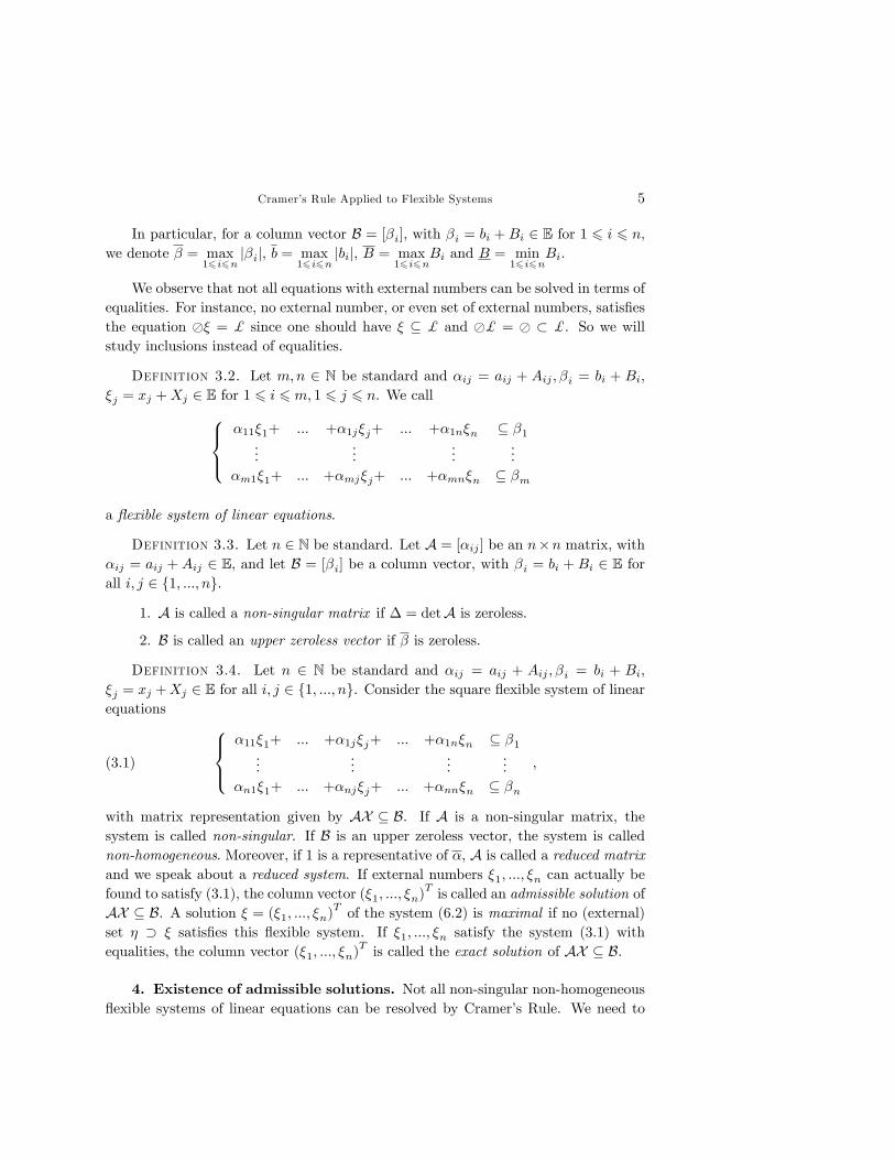
We observe that not all equations with external numbers can be solved in terms ofequalities. For instance, no external number, or even set of external numbers, satis�esthe equation �� = $ since one should have � � $ and �$ = � � $. So we willstudy inclusions instead of equalities.
Definition 3.2. Let m;n 2 N be standard and �ij = aij + Aij ; �i = bi + Bi;
�j = xj +Xj 2 E for 1 6 i 6 m; 1 6 j 6 n. We call8><>:�11�1+ ::: +�1j�j+ ::: +�1n�n � �1...
......
...�m1�1+ ::: +�mj�j+ ::: +�mn�n � �m
a �exible system of linear equations.
Definition 3.3. Let n 2 N be standard. Let A = [�ij ] be an n�n matrix, with�ij = aij + Aij 2 E; and let B = [�i] be a column vector, with �i = bi + Bi 2 E forall i; j 2 f1; :::; ng.
1. A is called a non-singular matrix if � = detA is zeroless.
2. B is called an upper zeroless vector if � is zeroless.
Definition 3.4. Let n 2 N be standard and �ij = aij + Aij ; �i = bi + Bi;
�j = xj +Xj 2 E for all i; j 2 f1; :::; ng. Consider the square �exible system of linearequations
(3.1)
8><>:�11�1+ ::: +�1j�j+ ::: +�1n�n � �1...
......
...�n1�1+ ::: +�nj�j+ ::: +�nn�n � �n
;
with matrix representation given by AX � B. If A is a non-singular matrix, thesystem is called non-singular. If B is an upper zeroless vector, the system is callednon-homogeneous. Moreover, if 1 is a representative of �, A is called a reduced matrixand we speak about a reduced system. If external numbers �1; :::; �n can actually befound to satisfy (3:1), the column vector (�1; :::; �n)
T is called an admissible solution ofAX � B. A solution � = (�1; :::; �n)
T of the system (6:2) is maximal if no (external)set � � � satis�es this �exible system. If �1; :::; �n satisfy the system (3:1) withequalities, the column vector (�1; :::; �n)
T is called the exact solution of AX � B.
4. Existence of admissible solutions. Not all non-singular non-homogeneous�exible systems of linear equations can be resolved by Cramer�s Rule. We need to
6 Júlia Justino and Imme van den Berg
control the uncertainties of the system in order to guarantee that Cramer�s Ruleproduces a valid solution and, if necessary, to make some adaptations. The matrix Aof coe¢ cients has to be more precise, in a sense, than the constant term vector B. Thegeneral theorem presented in this section shows that, under certain conditions uponthe size of the uncertainties appearing in a non-singular non-homogeneous �exiblesystem of linear equations, it is possible to guarantee the existence of admissiblesolutions by Cramer�s Rule. Even when not all of those conditions are satis�ed itis still possible, in some cases, to obtain an admissible solution given by adaptingCramer�s Rule, where we neglect some uncertainties of the system.
In this section we will simply call a non-singular non-homogeneous �exible sys-tem of linear equations �exible system and a reduced non-singular non-homogeneous�exible system of linear equations reduced �exible system.
We start by de�ning the kind of precision needed in order to control the uncer-tainties appearing in a �exible system.
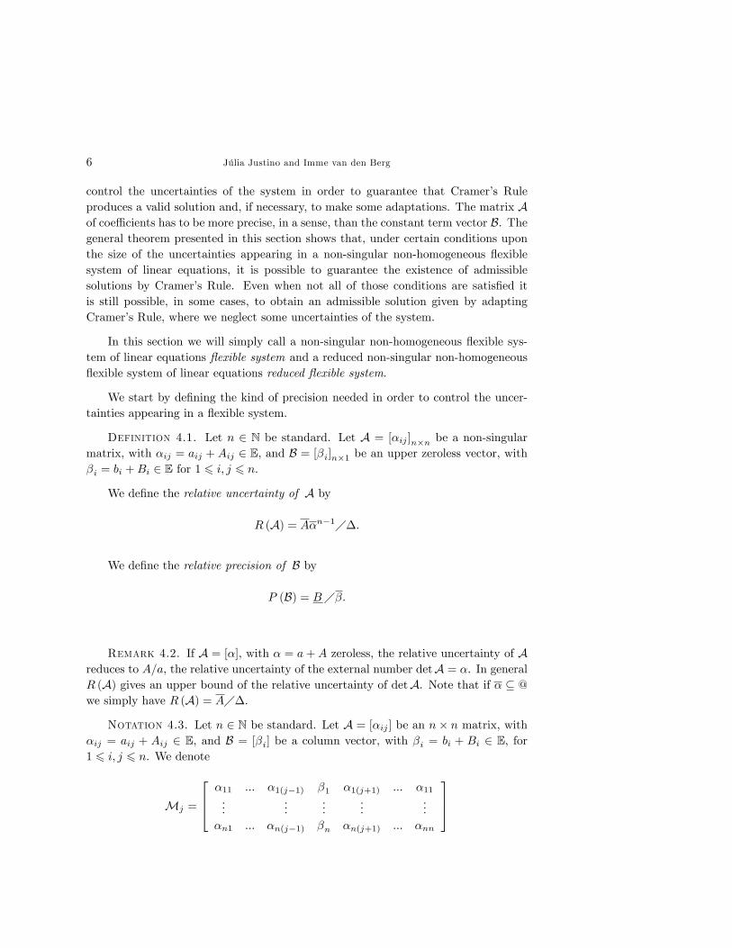
Definition 4.1. Let n 2 N be standard. Let A = [�ij ]n�n be a non-singularmatrix, with �ij = aij + Aij 2 E, and B = [�i]n�1 be an upper zeroless vector, with�i = bi +Bi 2 E for 1 6 i; j 6 n.
We de�ne the relative uncertainty of A by
R (A) = A�n�1��:
We de�ne the relative precision of B by
P (B) = B��:
Remark 4.2. If A = [�], with � = a+ A zeroless, the relative uncertainty of Areduces to A=a, the relative uncertainty of the external number detA = �. In generalR (A) gives an upper bound of the relative uncertainty of detA. Note that if � � @we simply have R (A) = A��.
Notation 4.3. Let n 2 N be standard. Let A = [�ij ] be an n� n matrix, with�ij = aij + Aij 2 E, and B = [�i] be a column vector, with �i = bi + Bi 2 E, for1 6 i; j 6 n. We denote
Mj =
264 �11 ::: �1(j�1) �1 �1(j+1) ::: �11...
......
......
�n1 ::: �n(j�1) �n �n(j+1) ::: �nn
375
Cramer�s Rule Applied to Flexible Systems 7
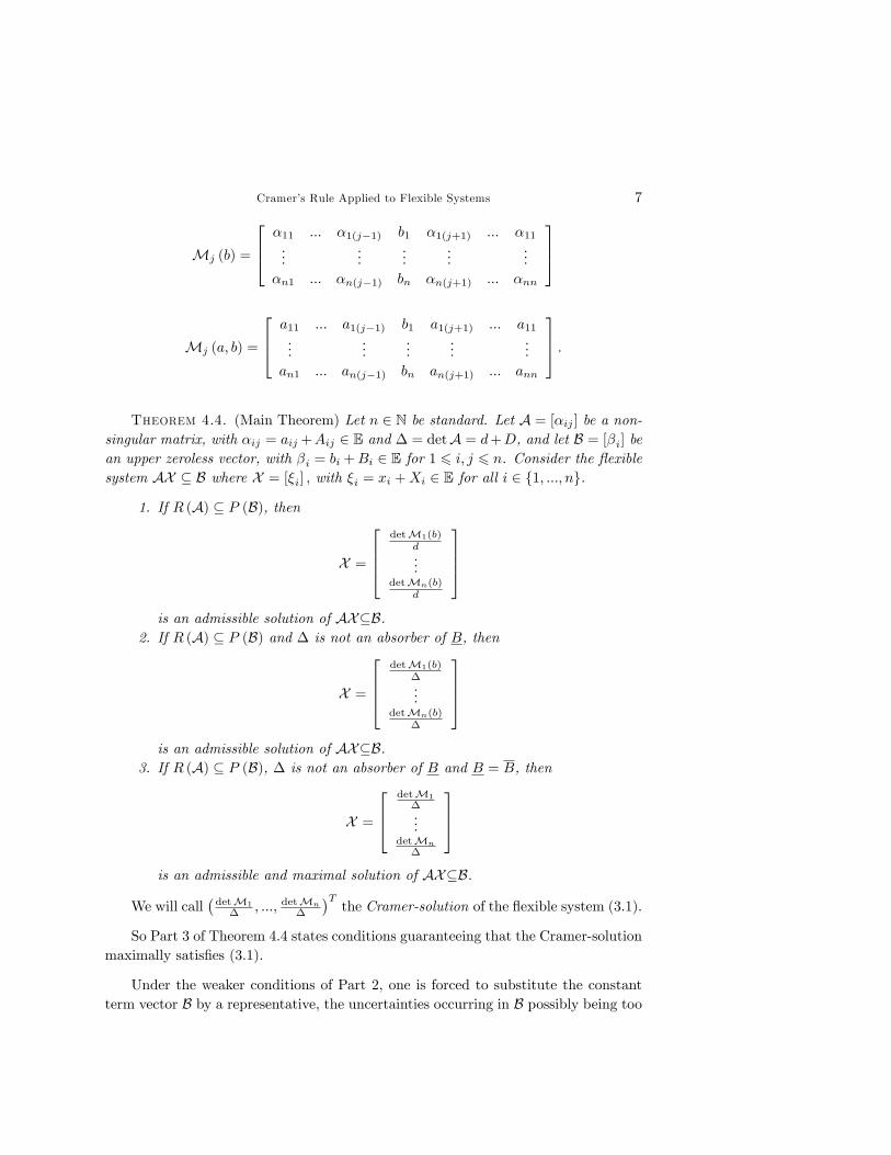
Mj (b) =
264 �11 ::: �1(j�1) b1 �1(j+1) ::: �11...
......
......
�n1 ::: �n(j�1) bn �n(j+1) ::: �nn
375
Mj (a; b) =
264 a11 ::: a1(j�1) b1 a1(j+1) ::: a11...
......
......
an1 ::: an(j�1) bn an(j+1) ::: ann
375 :
Theorem 4.4. (Main Theorem) Let n 2 N be standard. Let A = [�ij ] be a non-singular matrix, with �ij = aij +Aij 2 E and � = detA = d+D, and let B = [�i] bean upper zeroless vector, with �i = bi +Bi 2 E for 1 6 i; j 6 n. Consider the �exiblesystem AX � B where X = [�i] ; with �i = xi +Xi 2 E for all i 2 f1; :::; ng.
1. If R (A) � P (B), then
X =
2664detM1(b)
d...
detMn(b)d
3775is an admissible solution of AX�B.
2. If R (A) � P (B) and � is not an absorber of B, then
X =
2664detM1(b)
�...
detMn(b)�
3775is an admissible solution of AX�B.
3. If R (A) � P (B), � is not an absorber of B and B = B, then
X =
264detM1
�...
detMn
�
375is an admissible and maximal solution of AX�B.
We will call�detM1
� ; :::; detMn
�
�Tthe Cramer-solution of the �exible system (3:1).
So Part 3 of Theorem 4.4 states conditions guaranteeing that the Cramer-solutionmaximally satis�es (3:1).
Under the weaker conditions of Part 2, one is forced to substitute the constantterm vector B by a representative, the uncertainties occurring in B possibly being too
8 Júlia Justino and Imme van den Berg
large. If only the condition on the relative precision R (A) � P (B) is known to hold,also the determinant � must be substituted by a representative. The condition that� should not be so small as to be an absorber of B may be seen, in a sense, as ageneralization of the usual condition on non-singularity of determinant of the matrixof coe¢ cients, i.e. that this determinant should be non-zero.
We show now some examples which illustrate the role of the conditions presentedin Theorem 4.4.
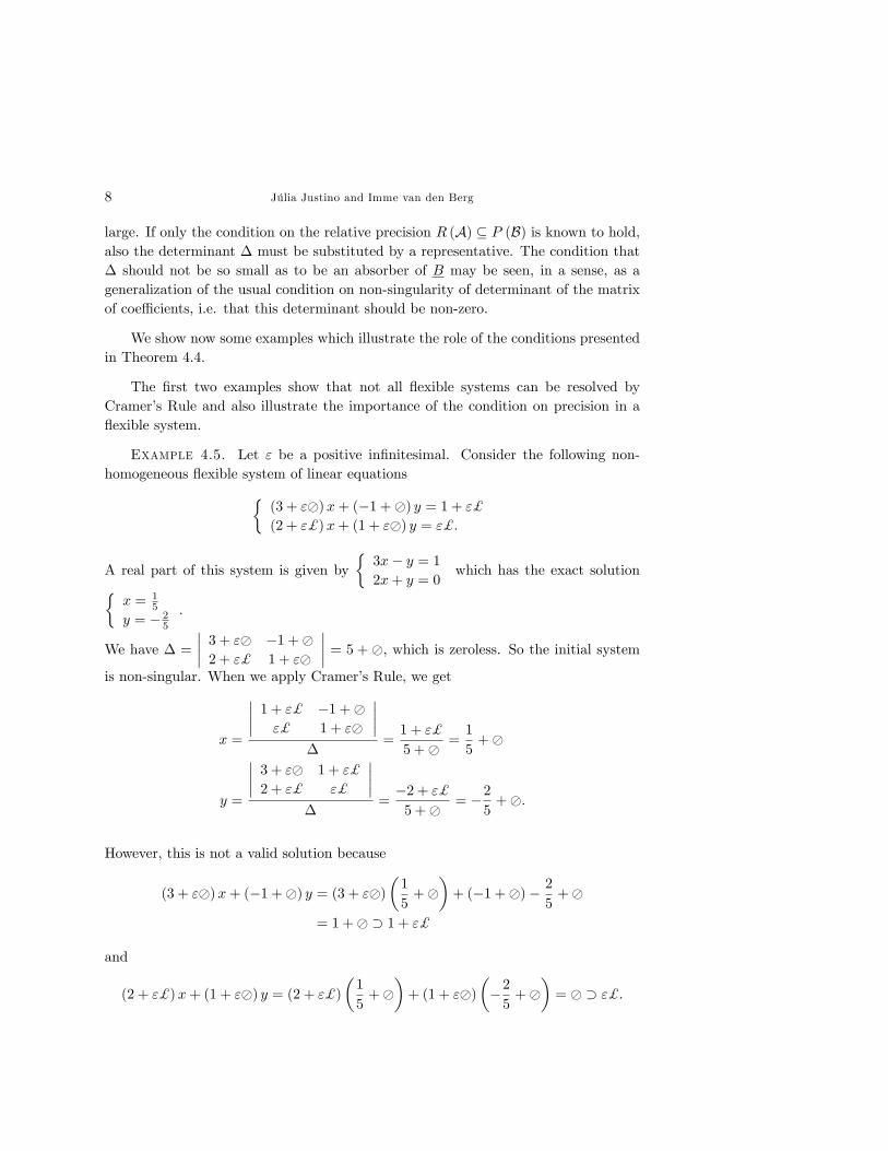
The �rst two examples show that not all �exible systems can be resolved byCramer�s Rule and also illustrate the importance of the condition on precision in a�exible system.
Example 4.5. Let " be a positive in�nitesimal. Consider the following non-homogeneous �exible system of linear equations�
(3 + "�)x+ (�1 +�) y = 1 + "$(2 + "$)x+ (1 + "�) y = "$:
A real part of this system is given by�3x� y = 12x+ y = 0
which has the exact solution�x = 1
5
y = � 25
.
We have � =
���� 3 + "� �1 +�2 + "$ 1 + "�
���� = 5 + �, which is zeroless. So the initial systemis non-singular. When we apply Cramer�s Rule, we get
x =
���� 1 + "$ �1 +�"$ 1 + "�
�����
=1 + "$
5 +� =1
5+�
y =
���� 3 + "� 1 + "$
2 + "$ "$
�����
=�2 + "$5 +� = �2
5+�:
However, this is not a valid solution because
(3 + "�)x+ (�1 +�) y = (3 + "�)�1
5+�
�+ (�1 +�)� 2
5+�
= 1 +� � 1 + "$
and
(2 + "$)x+ (1 + "�) y = (2 + "$)�1
5+�
�+ (1 + "�)
��25+�
�= � � "$:
Cramer�s Rule Applied to Flexible Systems 9
In fact, using representatives, it is easy to show that this system does not have solu-tions at all.We have R (A) = A��� = 3�
5+� = � and P (B) = B�� = "$1+"$ = "$. So
R (A) " P (B) and Theorem 4.4 cannot be applied, although � is not an absorber ofB, since �B = "$ = B, and B = B = "$.
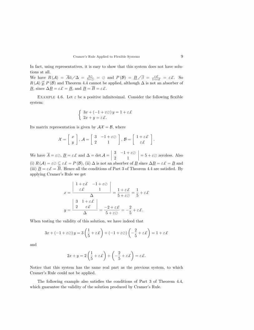
Example 4.6. Let " be a positive in�nitesimal. Consider the following �exiblesystem: �
3x+ (�1 + "�) y = 1 + "$2x+ y = "$:
Its matrix representation is given by AX = B, where
X =
�x
y
�, A =
�3 �1 + "�2 1
�, B =
�1 + "$
"$
�:
We have A = "�; B = "$ and � = detA =���� 3 �1 + "�2 1
���� = 5 + "� zeroless. Also(i) R (A) = "� � "$ = P (B), (ii) � is not an absorber of B since �B = "$ = B and(iii) B = "$ = B. Hence all the conditions of Part 3 of Theorem 4.4 are satis�ed. Byapplying Cramer�s Rule we get
x =
���� 1 + "$ �1 + "�"$ 1
�����
=1 + "$
5 + "� =1
5+ "$
y =
���� 3 1 + "$
2 "$
�����
=�2 + "$5 + "� = �2
5+ "$:
When testing the validity of this solution, we have indeed that
3x+ (�1 + "�) y = 3�1
5+ "$
�+ (�1 + "�)
��25+ "$
�= 1 + "$
and
2x+ y = 2
�1
5+ "$
�+
��25+ "$
�= "$:
Notice that this system has the same real part as the previous system, to whichCramer�s Rule could not be applied.
The following example also satis�es the conditions of Part 3 of Theorem 4.4,which guarantee the validity of the solution produced by Cramer�s Rule.
10 Júlia Justino and Imme van den Berg
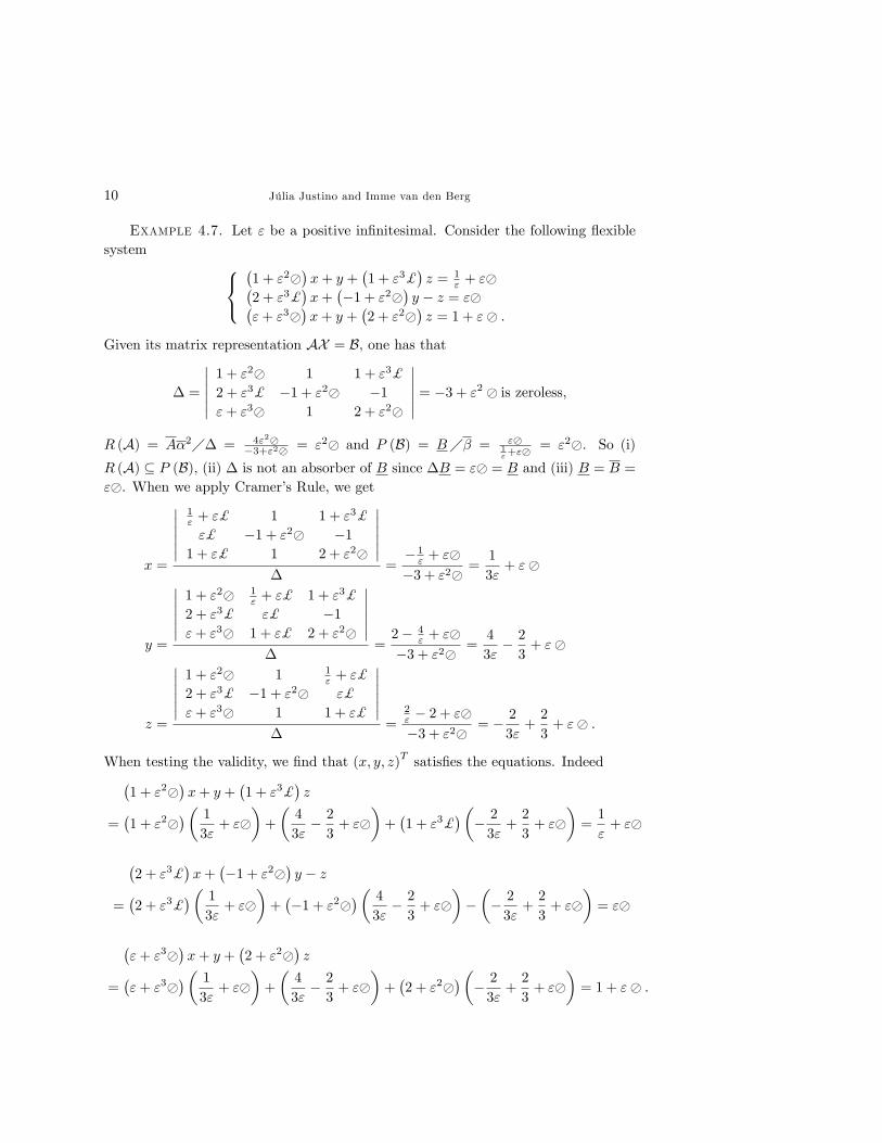
Example 4.7. Let " be a positive in�nitesimal. Consider the following �exiblesystem 8<:
�1 + "2�
�x+ y +
�1 + "3$
�z = 1
" + "��2 + "3$
�x+
��1 + "2�
�y � z = "��
"+ "3��x+ y +
�2 + "2�
�z = 1 + "� :
Given its matrix representation AX = B, one has that
� =
������1 + "2� 1 1 + "3$
2 + "3$ �1 + "2� �1"+ "3� 1 2 + "2�
������ = �3 + "2 � is zeroless,R (A) = A�2�� = 4"2�
�3+"2� = "2� and P (B) = B�� = "�1"+"�
= "2�. So (i)R (A) � P (B), (ii) � is not an absorber of B since �B = "� = B and (iii) B = B ="�. When we apply Cramer�s Rule, we get
x =
������1" + "$ 1 1 + "3$
"$ �1 + "2� �11 + "$ 1 2 + "2�
�������
=� 1" + "�
�3 + "2� =1
3"+ "�
y =
������1 + "2� 1
" + "$ 1 + "3$
2 + "3$ "$ �1"+ "3� 1 + "$ 2 + "2�
�������
=2� 4
" + "��3 + "2� =
4
3"� 23+ "�
z =
������1 + "2� 1 1
" + "$
2 + "3$ �1 + "2� "$
"+ "3� 1 1 + "$
�������
=2" � 2 + "��3 + "2� = � 2
3"+2
3+ "� :
When testing the validity, we �nd that (x; y; z)T satis�es the equations. Indeed�1 + "2�
�x+ y +
�1 + "3$
�z
=�1 + "2�
�� 13"+ "�
�+
�4
3"� 23+ "�
�+�1 + "3$
��� 2
3"+2
3+ "�
�=1
"+ "�
�2 + "3$
�x+
��1 + "2�
�y � z
=�2 + "3$
�� 13"+ "�
�+��1 + "2�
�� 43"� 23+ "�
���� 2
3"+2
3+ "�
�= "�
�"+ "3�
�x+ y +
�2 + "2�
�z
=�"+ "3�
�� 13"+ "�
�+
�4
3"� 23+ "�
�+�2 + "2�
��� 2
3"+2
3+ "�
�= 1 + "� :
Cramer�s Rule Applied to Flexible Systems 11
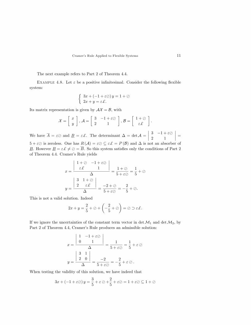
The next example refers to Part 2 of Theorem 4.4.
Example 4.8. Let " be a positive in�nitesimal. Consider the following �exiblesystem: �
3x+ (�1 + "�) y = 1 +�2x+ y = "$:
Its matrix representation is given by AX = B, with
X =
�x
y
�, A =
�3 �1 + "�2 1
�, B =
�1 +�"$
�:
We have A = "� and B = "$. The determinant � = detA =
���� 3 �1 + "�2 1
���� =5 + "� is zeroless. One has R (A) = "� � "$ = P (B) and � is not an absorber ofB. However B = "$ 6= � = B. So this system satis�es only the conditions of Part 2of Theorem 4.4. Cramer�s Rule yields
x =
���� 1 +� �1 + "�"$ 1
�����
=1 +�5 + "� =
1
5+�
y =
���� 3 1 +�2 "$
�����
=�2 +�5 + "� = �2
5+�:
This is not a valid solution. Indeed
2x+ y =2
5+�+
��25+�
�= � � "$:
If we ignore the uncertainties of the constant term vector in detM1 and detM2, byPart 2 of Theorem 4.4, Cramer�s Rule produces an admissible solution:
x =
���� 1 �1 + "�0 1
�����
=1
5 + "� =1
5+ "�
y =
���� 3 1
2 0
�����
=�2
5 + "� = �25+ "� :
When testing the validity of this solution, we have indeed that
3x+ (�1 + "�) y = 3
5+ "�+2
5+ "� = 1 + "� � 1 +�
12 Júlia Justino and Imme van den Berg
and
2x+ y =2
5+ "��2
5+ "� = "� � "$:
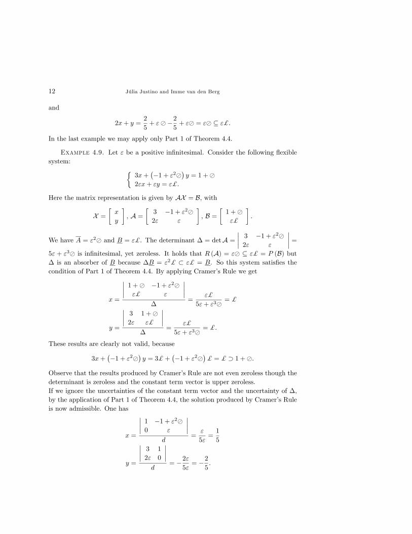
In the last example we may apply only Part 1 of Theorem 4.4.
Example 4.9. Let " be a positive in�nitesimal. Consider the following �exiblesystem: �
3x+��1 + "2�
�y = 1 +�
2"x+ "y = "$:
Here the matrix representation is given by AX = B, with
X =
�x
y
�, A =
�3 �1 + "2�2" "
�, B =
�1 +�"$
�:
We have A = "2� and B = "$. The determinant � = detA =���� 3 �1 + "2�2" "
���� =5" + "3� is in�nitesimal, yet zeroless. It holds that R (A) = "� � "$ = P (B) but� is an absorber of B because �B = "2$ � "$ = B. So this system satis�es thecondition of Part 1 of Theorem 4.4. By applying Cramer�s Rule we get
x =
���� 1 +� �1 + "2�"$ "
�����
="$
5"+ "3� = $
y =
���� 3 1 +�2" "$
�����
="$
5"+ "3� = $:
These results are clearly not valid, because
3x+��1 + "2�
�y = 3$+
��1 + "2�
�$ = $ � 1 +�:
Observe that the results produced by Cramer�s Rule are not even zeroless though thedeterminant is zeroless and the constant term vector is upper zeroless.If we ignore the uncertainties of the constant term vector and the uncertainty of �,by the application of Part 1 of Theorem 4.4, the solution produced by Cramer�s Ruleis now admissible. One has
x =
���� 1 �1 + "2�0 "
����d
="
5"=1
5
y =
���� 3 1
2" 0
����d
= �2"5"= �2
5:
Cramer�s Rule Applied to Flexible Systems 13
When testing the validity of this solution, we have indeed that
3x+��1 + "2�
�y =
3
5� 25
��1 + "2�
�= 1 + "2� � 1 +�
and
2"x+ "y =2"
5� 2"5= 0 � "$:
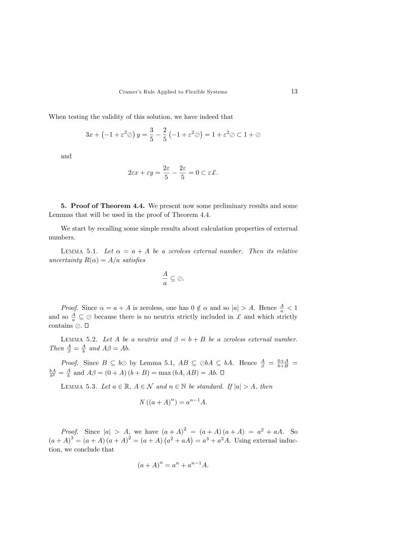
5. Proof of Theorem 4.4. We present now some preliminary results and someLemmas that will be used in the proof of Theorem 4.4.
We start by recalling some simple results about calculation properties of externalnumbers.
Lemma 5.1. Let � = a + A be a zeroless external number. Then its relativeuncertainty R(�) = A=a satis�es
A
a� �:
Proof. Since � = a + A is zeroless, one has 0 =2 � and so jaj > A. Hence Aa < 1
and so Aa � � because there is no neutrix strictly included in $ and which strictly
contains �.
Lemma 5.2. Let A be a neutrix and � = b + B be a zeroless external number.Then A
� =Ab and A� = Ab:
Proof. Since B � b� by Lemma 5.1, AB � �bA � bA. Hence A� = 0+A
b+B =bAb2 =
Ab and A� = (0 +A) (b+B) = max (bA;AB) = Ab.
Lemma 5.3. Let a 2 R, A 2 N and n 2 N be standard. If jaj > A, then
N ((a+A)n) = an�1A:
Proof. Since jaj > A, we have (a+A)2 = (a+A) (a+A) = a2 + aA. So(a+A)
3= (a+A) (a+A)
2= (a+A)
�a2 + aA
�= a3 + a2A. Using external induc-
tion, we conclude that
(a+A)n= an + an�1A:
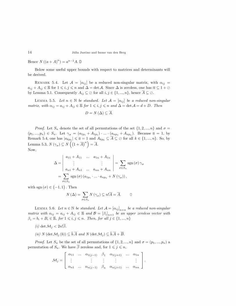
14 Júlia Justino and Imme van den Berg
Hence N ((a+A)n) = an�1A:
Below some useful upper bounds with respect to matrices and determinants willbe derived.
Remark 5.4. Let A = [�ij ] be a reduced non-singular matrix, with �ij =aij +Aij 2 E for 1 6 i; j 6 n and � = detA. Since � is zeroless, one has � � 1 +�by Lemma 5.1. Consequently Aij � � for all i; j 2 f1; :::; ng, hence A � �:
Lemma 5.5. Let n 2 N be standard. Let A = [�ij ] be a reduced non-singularmatrix, with �ij = aij +Aij 2 E for 1 6 i; j 6 n and � = detA = d+D. Then
D = N (�) � A:
Proof. Let Sn denote the set of all permutations of the set f1; 2; :::; ng and � =(p1; :::; pn) 2 Sn. Let � = (a1p1 +A1p1) � ::: � (anpn +Anpn). Because a = 1, byRemark 5.4, one has jakpk j 6 a = 1 and Akpk � A � � for all k 2 f1; :::; ng. So, byLemma 5.3, N ( �) � N
��1 +A
�n�= A.
Now,
� =
�������a11 +A11 ::: a1n +A1n
......
an1 +An1 ::: ann +Ann
������� =X�2Sn
sgn (�) �
=X�2Sn
sgn (�) (a1p1 � ::: � anpn +N ( �)) ;
with sgn (�) 2 f�1; 1g : Then
N (�) =X�2Sn
N ( �) � n!A = A:
Lemma 5.6. Let n 2 N be standard. Let A = [�ij ]n�n be a reduced non-singularmatrix with �ij = aij + Aij 2 E and B = [�i]n�1 be an upper zeroless vector with�i = bi +Bi 2 E, for 1 6 i; j 6 n. Then, for all j 2 f1; :::; ng
(i) detMj < 2n!�:
(ii) N (detMj (b)) � b:A and N (detMj) � b:A+B:
Proof. Let Sn be the set of all permutations of f1; 2; :::; ng and � = (p1; :::; pn) apermutation of Sn. We have � zeroless and, for 1 6 j 6 n,
Mj =
264 �11 ::: �1(j�1) �1 �1(j+1) ::: �1n...
......
......
�n1 ::: �n(j�1) �n �n(j+1) ::: �nn
375 :
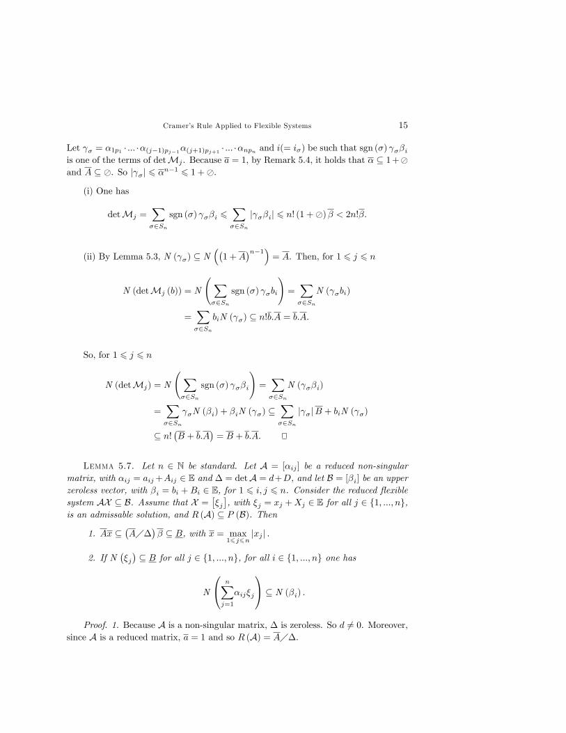
Cramer�s Rule Applied to Flexible Systems 15
Let � = �1p1 � ::: ��(j�1)pj�1�(j+1)pj+1 � ::: ��npn and i(= i�) be such that sgn (�) ��iis one of the terms of detMj . Because a = 1, by Remark 5.4, it holds that � � 1+�and A � �. So j �j 6 �n�1 6 1 +�.
(i) One has
detMj =X�2Sn
sgn (�) ��i 6X�2Sn
j ��ij 6 n! (1 +�)� < 2n!�:
(ii) By Lemma 5.3, N ( �) � N��1 +A
�n�1�= A. Then, for 1 6 j 6 n
N (detMj (b)) = N
X�2Sn
sgn (�) �bi
!=X�2Sn
N ( �bi)
=X�2Sn
biN ( �) � n!b:A = b:A:
So, for 1 6 j 6 n
N (detMj) = N
X�2Sn
sgn (�) ��i
!=X�2Sn
N ( ��i)
=X�2Sn
�N (�i) + �iN ( �) �X�2Sn
j �jB + biN ( �)
� n!�B + b:A
�= B + b:A:
Lemma 5.7. Let n 2 N be standard. Let A = [�ij ] be a reduced non-singularmatrix, with �ij = aij+Aij 2 E and � = detA = d+D, and let B = [�i] be an upperzeroless vector, with �i = bi +Bi 2 E, for 1 6 i; j 6 n. Consider the reduced �exiblesystem AX � B. Assume that X =
��j�, with �j = xj +Xj 2 E for all j 2 f1; :::; ng,
is an admissable solution, and R (A) � P (B). Then
1. Ax ��A��
�� � B, with x = max
16j6njxj j :
2. If N��j�� B for all j 2 f1; :::; ng, for all i 2 f1; :::; ng one has
N
0@ nXj=1
�ij�j
1A � N (�i) :
Proof. 1. Because A is a non-singular matrix, � is zeroless. So d 6= 0. Moreover,since A is a reduced matrix, a = 1 and so R (A) = A��.
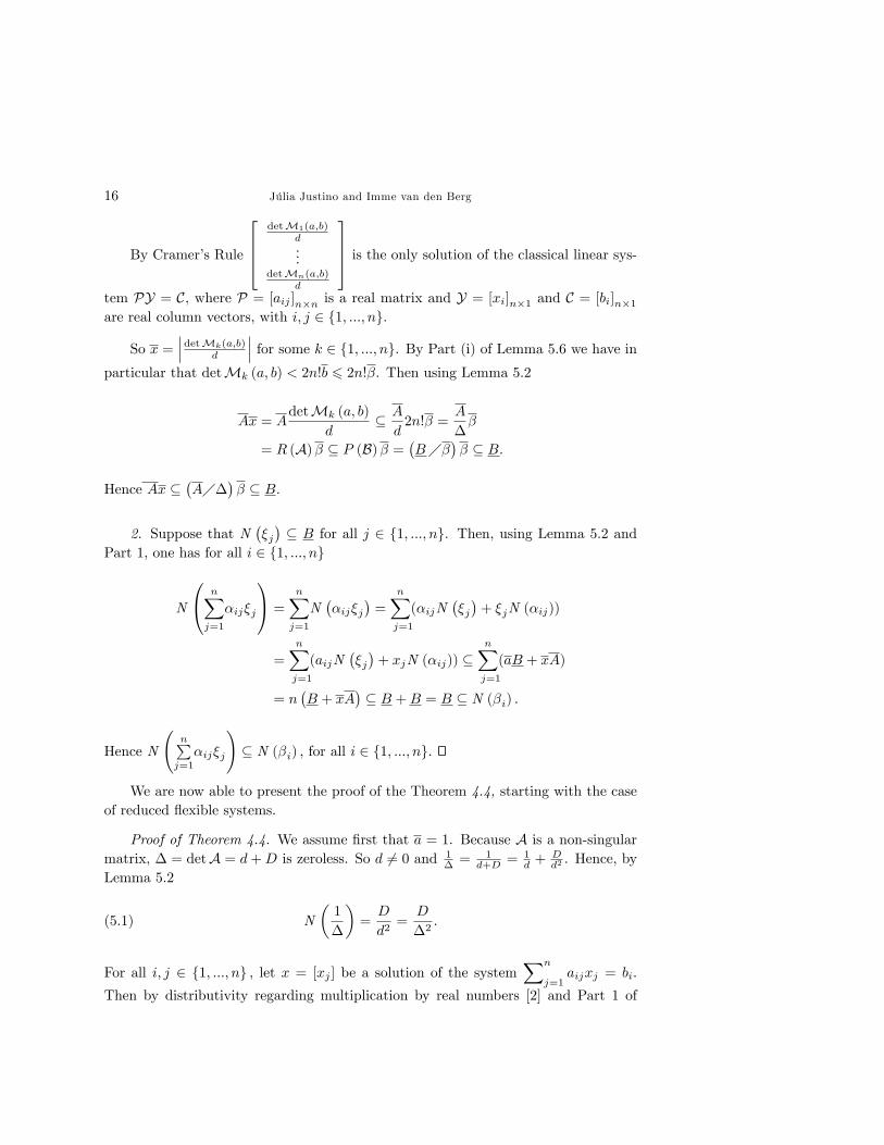
16 Júlia Justino and Imme van den Berg
By Cramer�s Rule
2664detM1(a;b)
d...
detMn(a;b)d
3775 is the only solution of the classical linear sys-tem PY = C, where P = [aij ]n�n is a real matrix and Y = [xi]n�1 and C = [bi]n�1are real column vectors, with i; j 2 f1; :::; ng.
So x =���detMk(a;b)
d
��� for some k 2 f1; :::; ng. By Part (i) of Lemma 5.6 we have inparticular that detMk (a; b) < 2n!b 6 2n!�. Then using Lemma 5.2
Ax = AdetMk (a; b)
d� A
d2n!� =
A
��
= R (A)� � P (B)� =�B��
�� � B:
Hence Ax ��A��
�� � B:
2. Suppose that N��j�� B for all j 2 f1; :::; ng. Then, using Lemma 5.2 and
Part 1, one has for all i 2 f1; :::; ng
N
0@ nXj=1
�ij�j
1A =
nXj=1
N��ij�j
�=
nX(
j=1
�ijN��j�+ �jN (�ij))
=nX(
j=1
aijN��j�+ xjN (�ij)) �
nX(
j=1
aB + xA)
= n�B + xA
�� B +B = B � N (�i) :
Hence N
nPj=1
�ij�j
!� N (�i) ; for all i 2 f1; :::; ng.
We are now able to present the proof of the Theorem 4.4, starting with the caseof reduced �exible systems.
Proof of Theorem 4.4. We assume �rst that a = 1. Because A is a non-singularmatrix, � = detA = d+D is zeroless. So d 6= 0 and 1
� =1
d+D = 1d +
Dd2 . Hence, by
Lemma 5.2
(5.1) N
�1
�
�=D
d2=D
�2:
For all i; j 2 f1; :::; ng ; let x = [xj ] be a solution of the systemXn
j=1aijxj = bi.
Then by distributivity regarding multiplication by real numbers [2] and Part 1 of
Cramer�s Rule Applied to Flexible Systems 17
Lemma 5.7
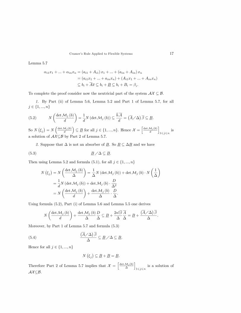
�i1x1 + :::+ �inxn = (ai1 +Ai1)x1 + :::+ (ain +Ain)xn
= (ai1x1 + :::+ ainxn) + (Ai1x1 + :::+Ainxn)
� bi +Ax � bi +B � bi +Bi = �i:
To complete the proof consider now the neutricial part of the system AX � B.
1. By Part (ii) of Lemma 5.6, Lemma 5.2 and Part 1 of Lemma 5.7, for allj 2 f1; :::; ng
(5.2) N
�detMj (b)
d
�=1
dN (detMj (b)) �
b:A
d=�A��
�� � B:
So N��j�= N
�detMj(b)
d
�� B for all j 2 f1; :::; ng. Hence X =
hdetMj(b)
d
i16j6n
is
a solution of AX�B by Part 2 of Lemma 5.7.
2. Suppose that � is not an absorber of B. So B � �B and we have
(5.3) B�� � B:
Then using Lemma 5.2 and formula (5.1), for all j 2 f1; :::; ng
N��j�= N
�detMj (b)
�
�=1
�N (detMj (b)) + detMj (b) �N
�1
�
�=1
dN (detMj (b)) + detMj (b) �
D
�2
= N
�detMj (b)
d
�+detMj (b)
�� D�:
Using formula (5.2), Part (i) of Lemma 5.6 and Lemma 5.5 one derives
N
�detMj (b)
d
�+detMj (b)
�
D
�� B + 2n!�
�
A
�= B +
�A��
��
�:
Moreover, by Part 1 of Lemma 5.7 and formula (5.3)
(5.4)
�A��
��
�� B�� � B:
Hence for all j 2 f1; :::; ng
N��j�� B +B = B:
Therefore Part 2 of Lemma 5.7 implies that X =hdetMj(b)
�
i16j6n
is a solution of
AX�B.
18 Júlia Justino and Imme van den Berg
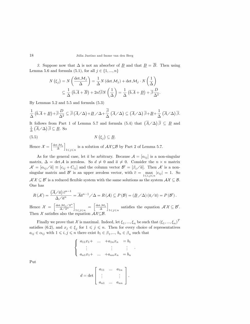
3. Suppose now that � is not an absorber of B and that B = B. Then usingLemma 5.6 and formula (5.1), for all j 2 f1; :::; ng
N��j�= N
�detMj
�
�=1
�N (detMj) + detMj �N
�1
�
�� 1
�
�b:A+B
�+ 2n!�N
�1
�
�=1
�
�b:A+B
�+ �
D
�2:
By Lemmas 5.2 and 5.5 and formula (5.3)
1
�
�b:A+B
�+�
D
�2� �
�A��
�+B��+
�
�
�A��
���A��
��+B+
1
�
�A��
��:
It follows from Part 1 of Lemma 5.7 and formula (5.4) that�A��
�� � B and
1�
�A��
�� � B. So
(5.5) N��j�� B:
Hence X =hdetMj
�
i16j6n
is a solution of AX�B by Part 2 of Lemma 5.7.
As for the general case, let a be arbitrary. Because A = [�ij ] is a non-singularmatrix, � = detA is zeroless. So d 6= 0 and a 6= 0. Consider the n � n matrixA0 = [�ij�a] � [cij + Cij ] and the column vector B0 = [�i�a]. Then A0 is a non-singular matrix and B0 is an upper zeroless vector, with c = max
16i;j6njcij j = 1. So
A0X � B0 is a reduced �exible system with the same solutions as the system AX � B.One has
R (A0) =�A�a
�cn�1
��an= Aan�1�� = R (A) � P (B) = (B��) (a�a) = P (B0) :
Hence X =hdetMj�an��an
i16j6n
=hdetMj
�
i16j6n
satis�es the equation A0X � B0.Then X satis�es also the equation AX�B.
Finally we prove that X is maximal. Indeed, let �1; :::; �n be such that (�1; :::; �n)T
satis�es (6:2), and xj 2 �j for 1 6 j 6 n. Then for every choice of representativesaij 2 �ij with 1 6 i; j 6 n there exist b1 2 �1,..., bn 2 �n such that8><>:
a11x1+ ::: +a1nxn = b1...
......
an1x1+ ::: +annxn = bn
:
Put
d = det
264 a11 ::: a1n...
...an1 ::: ann
375 :
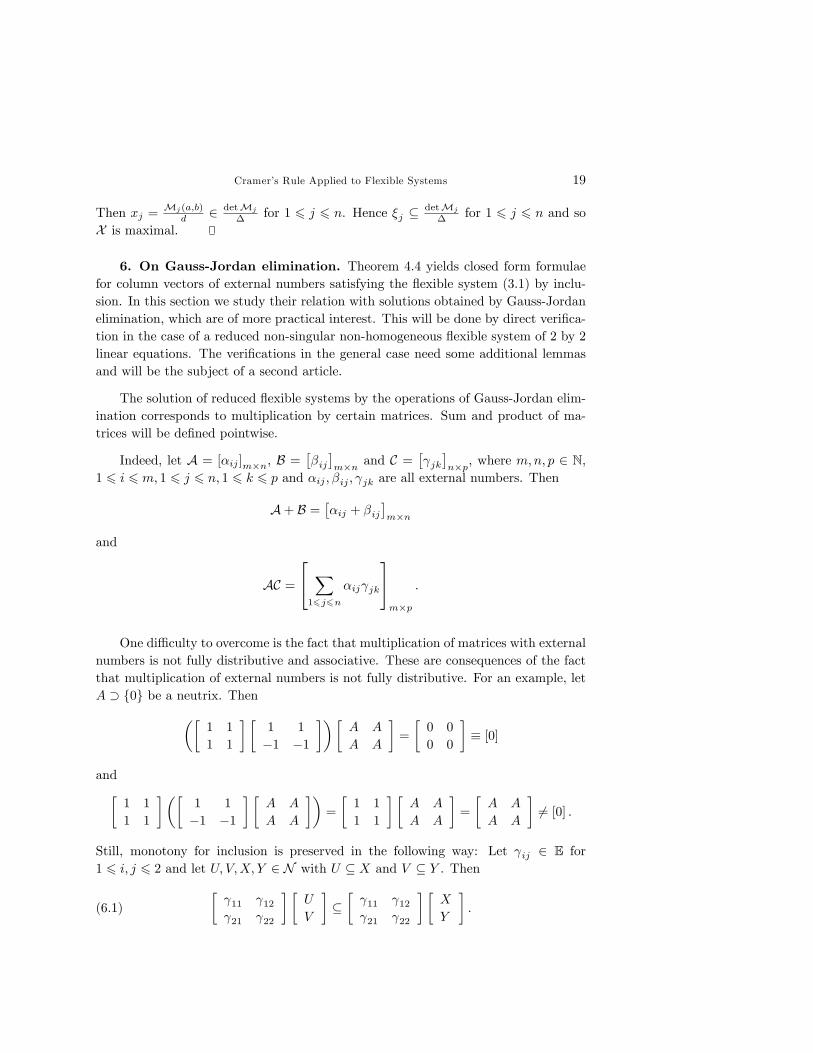
Cramer�s Rule Applied to Flexible Systems 19
Then xj =Mj(a;b)
d 2 detMj
� for 1 6 j 6 n. Hence �j �detMj
� for 1 6 j 6 n and soX is maximal.
6. On Gauss-Jordan elimination. Theorem 4.4 yields closed form formulaefor column vectors of external numbers satisfying the �exible system (3:1) by inclu-sion. In this section we study their relation with solutions obtained by Gauss-Jordanelimination, which are of more practical interest. This will be done by direct veri�ca-tion in the case of a reduced non-singular non-homogeneous �exible system of 2 by 2linear equations. The veri�cations in the general case need some additional lemmasand will be the subject of a second article.
The solution of reduced �exible systems by the operations of Gauss-Jordan elim-ination corresponds to multiplication by certain matrices. Sum and product of ma-trices will be de�ned pointwise.
Indeed, let A = [�ij ]m�n, B =��ij�m�n and C =
� jk�n�p, where m;n; p 2 N,
1 6 i 6 m; 1 6 j 6 n; 1 6 k 6 p and �ij ; �ij ; jk are all external numbers. Then
A+ B =��ij + �ij
�m�n
and
AC =
24 X16j6n
�ij jk
35m�p
:
One di¢ culty to overcome is the fact that multiplication of matrices with externalnumbers is not fully distributive and associative. These are consequences of the factthat multiplication of external numbers is not fully distributive. For an example, letA � f0g be a neutrix. Then��
1 1
1 1
� �1 1
�1 �1
���A A
A A
�=
�0 0
0 0
�� [0]
and�1 1
1 1
���1 1
�1 �1
� �A A
A A
��=
�1 1
1 1
� �A A
A A
�=
�A A
A A
�6= [0] :
Still, monotony for inclusion is preserved in the following way: Let ij 2 E for1 6 i; j 6 2 and let U; V;X; Y 2 N with U � X and V � Y . Then
(6.1)� 11 12 21 22
� �U
V
��� 11 12 21 22
� �X
Y
�:
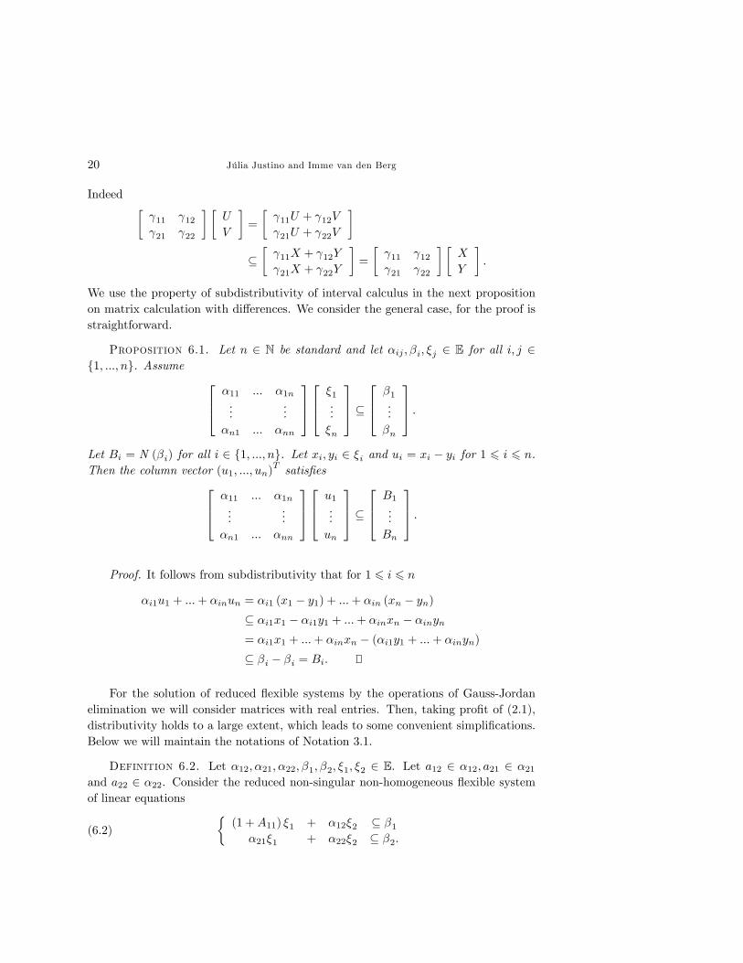
20 Júlia Justino and Imme van den Berg
Indeed � 11 12 21 22
� �U
V
�=
� 11U + 12V
21U + 22V
��� 11X + 12Y
21X + 22Y
�=
� 11 12 21 22
� �X
Y
�:
We use the property of subdistributivity of interval calculus in the next propositionon matrix calculation with di¤erences. We consider the general case, for the proof isstraightforward.
Proposition 6.1. Let n 2 N be standard and let �ij ; �i; �j 2 E for all i; j 2f1; :::; ng. Assume 264 �11 ::: �1n
......
�n1 ::: �nn
375264 �1
...�n
375 �264 �1
...�n
375 :Let Bi = N (�i) for all i 2 f1; :::; ng. Let xi; yi 2 �i and ui = xi � yi for 1 6 i 6 n.Then the column vector (u1; :::; un)
T satis�es264 �11 ::: �1n...
...�n1 ::: �nn
375264 u1
...un
375 �264 B1
...Bn
375 :
Proof. It follows from subdistributivity that for 1 6 i 6 n
�i1u1 + :::+ �inun = �i1 (x1 � y1) + :::+ �in (xn � yn)� �i1x1 � �i1y1 + :::+ �inxn � �inyn= �i1x1 + :::+ �inxn � (�i1y1 + :::+ �inyn)� �i � �i = Bi:
For the solution of reduced �exible systems by the operations of Gauss-Jordanelimination we will consider matrices with real entries. Then, taking pro�t of (2.1),distributivity holds to a large extent, which leads to some convenient simpli�cations.Below we will maintain the notations of Notation 3.1.
Definition 6.2. Let �12; �21; �22; �1; �2; �1; �2 2 E. Let a12 2 �12; a21 2 �21and a22 2 �22. Consider the reduced non-singular non-homogeneous �exible systemof linear equations
(6.2)�(1 +A11) �1 + �12�2 � �1�21�1 + �22�2 � �2:
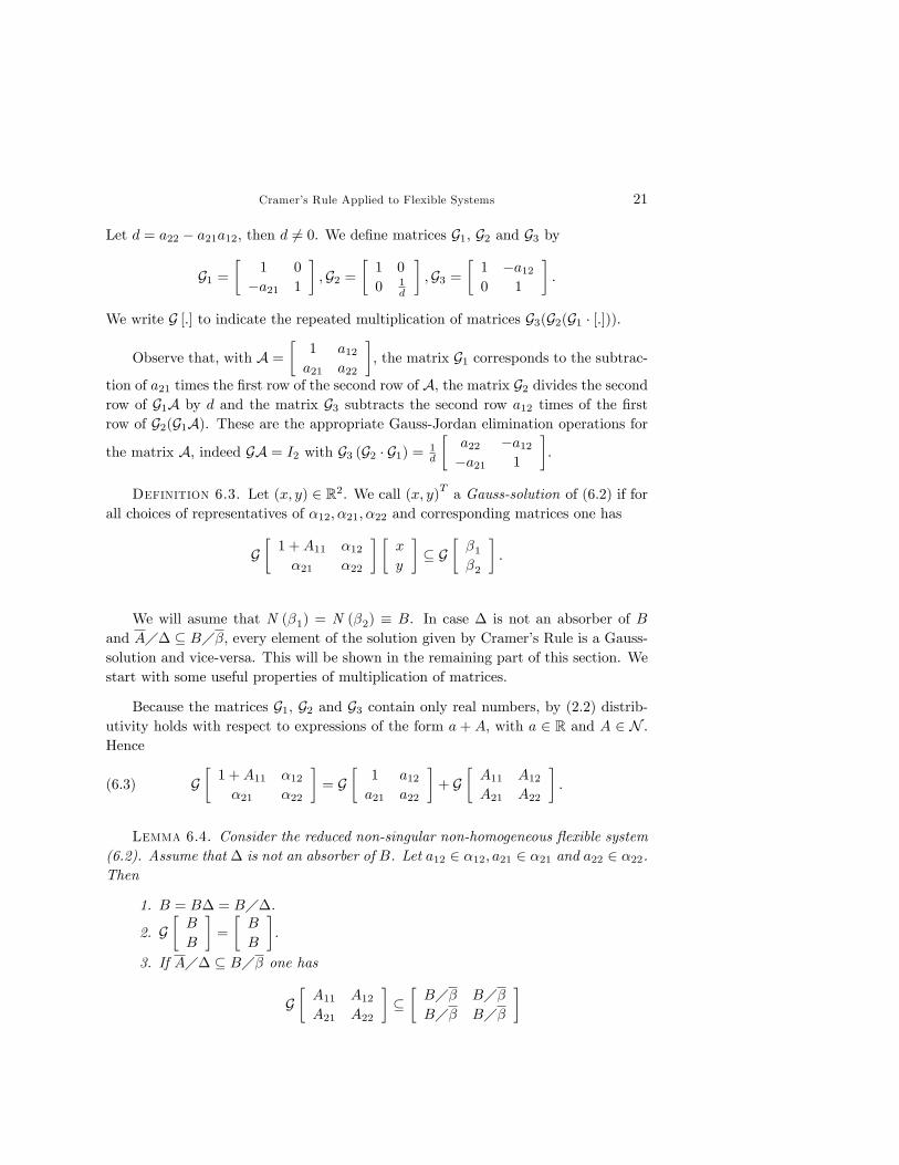
Cramer�s Rule Applied to Flexible Systems 21
Let d = a22 � a21a12, then d 6= 0. We de�ne matrices G1, G2 and G3 by
G1 =�
1 0
�a21 1
�;G2 =
�1 0
0 1d
�;G3 =
�1 �a120 1
�:
We write G [:] to indicate the repeated multiplication of matrices G3(G2(G1 � [:])).
Observe that, with A =�1 a12a21 a22
�, the matrix G1 corresponds to the subtrac-
tion of a21 times the �rst row of the second row of A, the matrix G2 divides the secondrow of G1A by d and the matrix G3 subtracts the second row a12 times of the �rstrow of G2(G1A). These are the appropriate Gauss-Jordan elimination operations for
the matrix A, indeed GA = I2 with G3 (G2 � G1) = 1d
�a22 �a12�a21 1
�.
Definition 6.3. Let (x; y) 2 R2. We call (x; y)T a Gauss-solution of (6:2) if forall choices of representatives of �12; �21; �22 and corresponding matrices one has
G�1 +A11 �12�21 �22
� �x
y
�� G
��1�2
�:
We will asume that N (�1) = N (�2) � B. In case � is not an absorber of Band A�� � B��, every element of the solution given by Cramer�s Rule is a Gauss-solution and vice-versa. This will be shown in the remaining part of this section. Westart with some useful properties of multiplication of matrices.
Because the matrices G1, G2 and G3 contain only real numbers, by (2.2) distrib-utivity holds with respect to expressions of the form a + A, with a 2 R and A 2 N .Hence
(6.3) G�1 +A11 �12�21 �22
�= G
�1 a12a21 a22
�+ G
�A11 A12A21 A22
�:
Lemma 6.4. Consider the reduced non-singular non-homogeneous �exible system(6.2). Assume that � is not an absorber of B. Let a12 2 �12; a21 2 �21 and a22 2 �22.Then
1. B = B� = B��.
2. G�B
B
�=
�B
B
�.
3. If A�� � B�� one has
G�A11 A12A21 A22
���B�� B��B�� B��
�
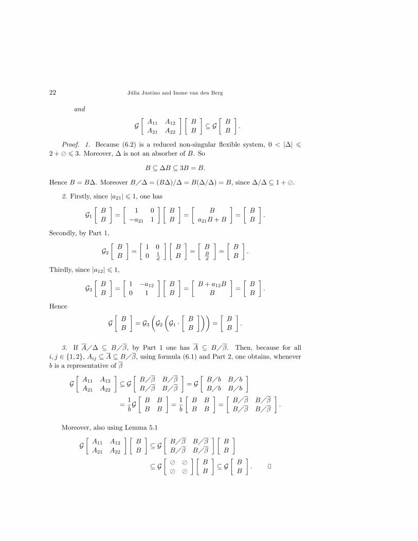
22 Júlia Justino and Imme van den Berg
and
G�A11 A12A21 A22
� �B
B
�� G
�B
B
�:
Proof. 1. Because (6:2) is a reduced non-singular �exible system, 0 < j�j 62 +� 6 3. Moreover, � is not an absorber of B. So
B � �B � 3B = B:
Hence B = B�. Moreover B�� = (B�)=� = B(�=�) = B, since �=� � 1 +�.
2. Firstly, since ja21j 6 1, one has
G1�B
B
�=
�1 0
�a21 1
� �B
B
�=
�B
a21B +B
�=
�B
B
�:
Secondly, by Part 1,
G2�B
B
�=
�1 0
0 1d
� �B
B
�=
�BBd
�=
�B
B
�:
Thirdly, since ja12j 6 1,
G3�B
B
�=
�1 �a120 1
� �B
B
�=
�B + a12B
B
�=
�B
B
�:
Hence
G�B
B
�= G3
�G2�G1 �
�B
B
���=
�B
B
�:
3. If A�� � B��, by Part 1 one has A � B��. Then, because for alli; j 2 f1; 2g, Aij � A � B��, using formula (6:1) and Part 2, one obtains, wheneverb is a representative of �
G�A11 A12A21 A22
�� G
�B�� B��B�� B��
�= G
�B�b B�bB�b B�b
�=1
bG�B B
B B
�=1
b
�B B
B B
�=
�B�� B��B�� B��
�:
Moreover, also using Lemma 5.1
G�A11 A12A21 A22
� �B
B
�� G
�B�� B��B�� B��
� �B
B
�� G
�� �� �
� �B
B
�� G
�B
B
�:
Cramer�s Rule Applied to Flexible Systems 23
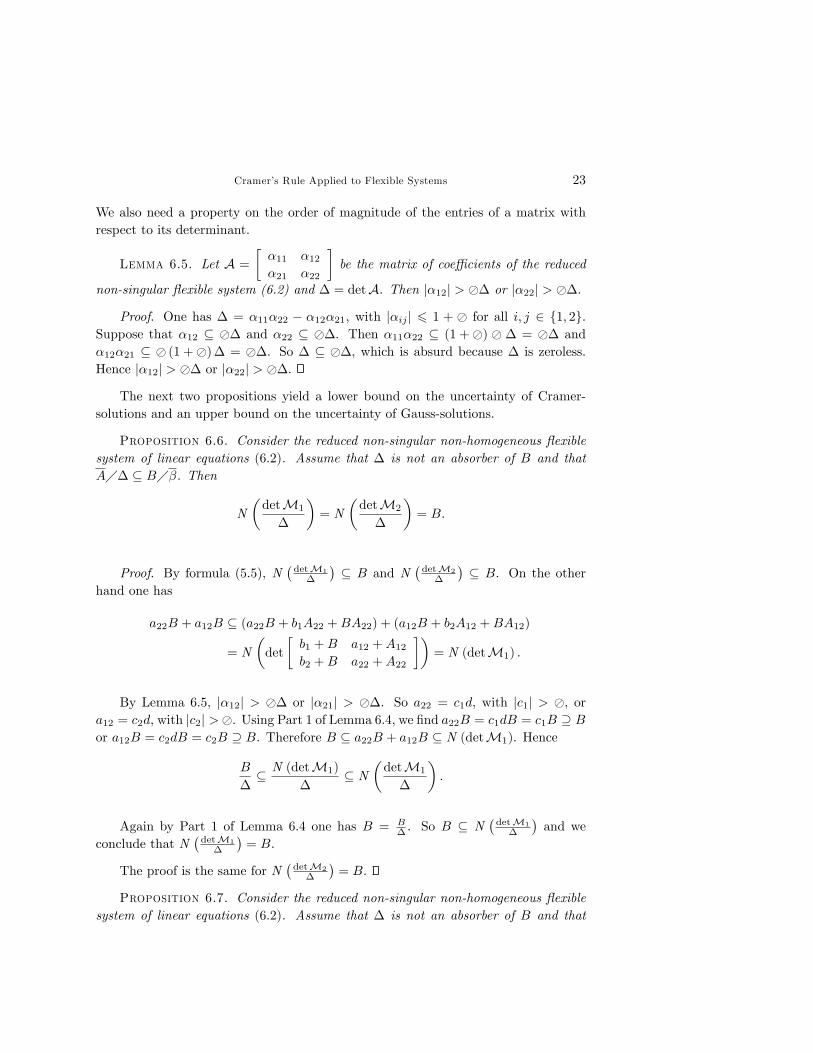
We also need a property on the order of magnitude of the entries of a matrix withrespect to its determinant.
Lemma 6.5. Let A =
��11 �12�21 �22
�be the matrix of coe¢ cients of the reduced
non-singular �exible system (6.2) and � = detA. Then j�12j > �� or j�22j > ��:
Proof. One has � = �11�22 � �12�21, with j�ij j 6 1 + � for all i; j 2 f1; 2g.Suppose that �12 � �� and �22 � ��. Then �11�22 � (1 +�) � � = �� and�12�21 � � (1 +�)� = ��. So � � ��, which is absurd because � is zeroless.Hence j�12j > �� or j�22j > ��.
The next two propositions yield a lower bound on the uncertainty of Cramer-solutions and an upper bound on the uncertainty of Gauss-solutions.
Proposition 6.6. Consider the reduced non-singular non-homogeneous �exiblesystem of linear equations (6:2). Assume that � is not an absorber of B and thatA�� � B��. Then
N
�detM1
�
�= N
�detM2
�
�= B:
Proof. By formula (5:5), N�detM1
�
�� B and N
�detM2
�
�� B. On the other
hand one has
a22B + a12B � (a22B + b1A22 +BA22) + (a12B + b2A12 +BA12)
= N
�det
�b1 +B a12 +A12b2 +B a22 +A22
��= N (detM1) :
By Lemma 6.5, j�12j > �� or j�21j > ��. So a22 = c1d, with jc1j > �, ora12 = c2d, with jc2j >�. Using Part 1 of Lemma 6.4, we �nd a22B = c1dB = c1B � Bor a12B = c2dB = c2B � B. Therefore B � a22B + a12B � N (detM1). Hence
B
�� N (detM1)
�� N
�detM1
�
�:
Again by Part 1 of Lemma 6.4 one has B = B� . So B � N
�detM1
�
�and we
conclude that N�detM1
�
�= B.
The proof is the same for N�detM2
�
�= B.
Proposition 6.7. Consider the reduced non-singular non-homogeneous �exiblesystem of linear equations (6:2). Assume that � is not an absorber of B and that
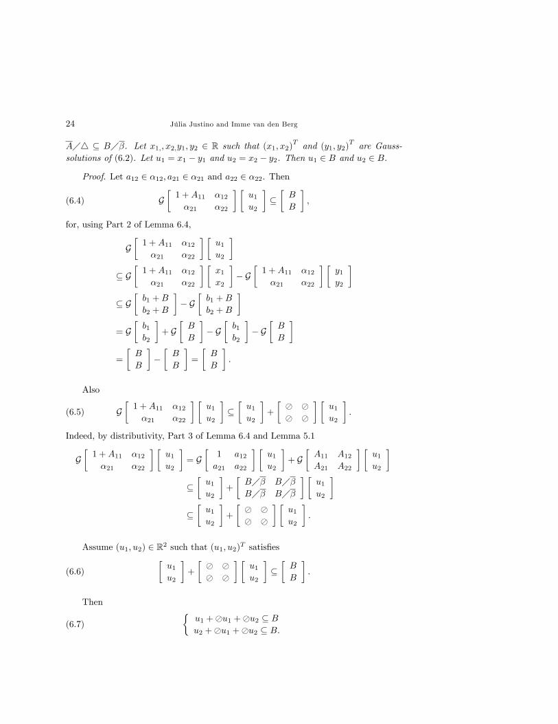
24 Júlia Justino and Imme van den Berg
A�4 � B��. Let x1;; x2;y1; y2 2 R such that (x1; x2)T and (y1; y2)
T are Gauss-solutions of (6:2). Let u1 = x1 � y1 and u2 = x2 � y2. Then u1 2 B and u2 2 B:
Proof. Let a12 2 �12; a21 2 �21 and a22 2 �22. Then
(6.4) G�1 +A11 �12�21 �22
� �u1u2
���B
B
�;
for, using Part 2 of Lemma 6.4,
G�1 +A11 �12�21 �22
� �u1u2
�� G
�1 +A11 �12�21 �22
� �x1x2
�� G
�1 +A11 �12�21 �22
� �y1y2
�� G
�b1 +B
b2 +B
�� G
�b1 +B
b2 +B
�= G
�b1b2
�+ G
�B
B
�� G
�b1b2
�� G
�B
B
�=
�B
B
���B
B
�=
�B
B
�:
Also
(6.5) G�1 +A11 �12�21 �22
� �u1u2
���u1u2
�+
�� �� �
� �u1u2
�:
Indeed, by distributivity, Part 3 of Lemma 6.4 and Lemma 5.1
G�1 +A11 �12�21 �22
� �u1u2
�= G
�1 a12a21 a22
� �u1u2
�+ G
�A11 A12A21 A22
� �u1u2
���u1u2
�+
�B�� B��B�� B��
� �u1u2
���u1u2
�+
�� �� �
� �u1u2
�:
Assume (u1; u2) 2 R2 such that (u1; u2)T satis�es
(6.6)�u1u2
�+
�� �� �
� �u1u2
���B
B
�:
Then
(6.7)�u1 +�u1 +�u2 � Bu2 +�u1 +�u2 � B:
Cramer�s Rule Applied to Flexible Systems 25
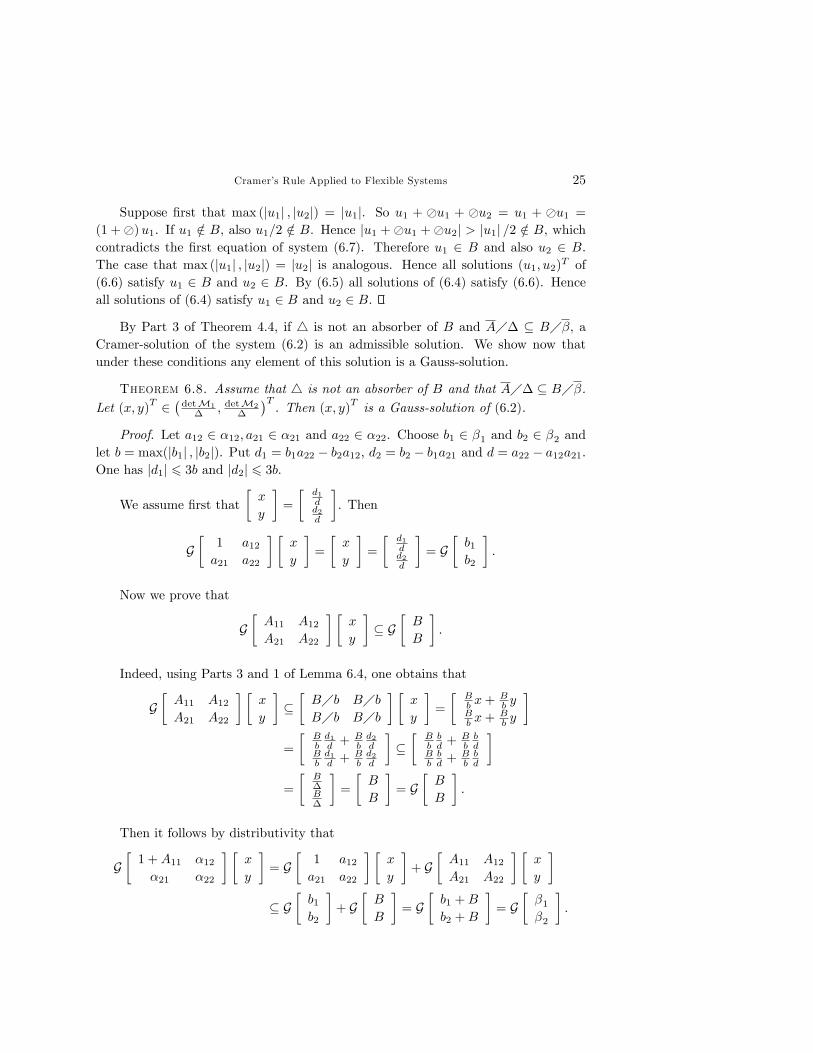
Suppose �rst that max (ju1j ; ju2j) = ju1j. So u1 + �u1 + �u2 = u1 + �u1 =(1 +�)u1. If u1 =2 B, also u1=2 =2 B. Hence ju1 +�u1 +�u2j > ju1j =2 =2 B, whichcontradicts the �rst equation of system (6.7). Therefore u1 2 B and also u2 2 B.The case that max (ju1j ; ju2j) = ju2j is analogous. Hence all solutions (u1; u2)T of(6.6) satisfy u1 2 B and u2 2 B. By (6.5) all solutions of (6.4) satisfy (6.6). Henceall solutions of (6.4) satisfy u1 2 B and u2 2 B.
By Part 3 of Theorem 4.4, if 4 is not an absorber of B and A�� � B��, aCramer-solution of the system (6:2) is an admissible solution. We show now thatunder these conditions any element of this solution is a Gauss-solution.
Theorem 6.8. Assume that 4 is not an absorber of B and that A�� � B��.Let (x; y)T 2
�detM1
� ; detM2
�
�T. Then (x; y)T is a Gauss-solution of (6:2).
Proof. Let a12 2 �12; a21 2 �21 and a22 2 �22. Choose b1 2 �1 and b2 2 �2 andlet b = max(jb1j ; jb2j). Put d1 = b1a22 � b2a12, d2 = b2 � b1a21 and d = a22 � a12a21.One has jd1j 6 3b and jd2j 6 3b.
We assume �rst that�x
y
�=
�d1dd2d
�. Then
G�1 a12a21 a22
� �x
y
�=
�x
y
�=
�d1dd2d
�= G
�b1b2
�:
Now we prove that
G�A11 A12A21 A22
� �x
y
�� G
�B
B
�:
Indeed, using Parts 3 and 1 of Lemma 6.4, one obtains that
G�A11 A12A21 A22
� �x
y
���B�b B�bB�b B�b
� �x
y
�=
�Bb x+
Bb y
Bb x+
Bb y
�=
�Bbd1d +
Bbd2d
Bbd1d +
Bbd2d
���
Bbbd +
Bbbd
Bbbd +
Bbbd
�=
�B�B�
�=
�B
B
�= G
�B
B
�:
Then it follows by distributivity that
G�1 +A11 �12�21 �22
� �x
y
�= G
�1 a12a21 a22
� �x
y
�+ G
�A11 A12A21 A22
� �x
y
�� G
�b1b2
�+ G
�B
B
�= G
�b1 +B
b2 +B
�= G
��1�2
�:
26 Júlia Justino and Imme van den Berg
Hence (x; y)T is a Gauss-solution of (6:2).
Finally, let�x0
y0
�2"
detM1
4detM2
4
#be arbitrary. By Proposition 6.6 one has
N�detM1
�
�= N
�detM2
�
�= B: So
�x0
y0
�2�x
y
�+
�B
B
�. Then by distributivity
and Lemma 6.4
G�1 +A11 �12�21 �22
� �x0
y0
�� G
�1 +A11 �12�21 �22
� �x
y
�+ G
�1 +A11 �12�21 �22
� �B
B
�� G
��1�2
�+ G
�1 a12a21 a22
� �B
B
�+ G
�A11 A12A21 A22
� �B
B
�� G
��1�2
�+
�B
B
�+ G
�B
B
�= G
��1�2
�+ G
�B
B
�+ G
�B
B
�= G
��1�2
�:
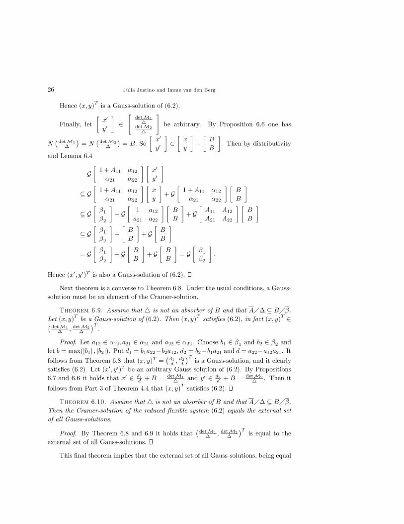
Hence (x0; y0)T is also a Gauss-solution of (6.2).
Next theorem is a converse to Theorem 6.8. Under the usual conditions, a Gauss-solution must be an element of the Cramer-solution.
Theorem 6.9. Assume that 4 is not an absorber of B and that A�� � B��.Let (x; y)T be a Gauss-solution of (6:2). Then (x; y)T satis�es (6:2), in fact (x; y)T 2�detM1
� ; detM2
�
�T.
Proof. Let a12 2 �12; a21 2 �21 and a22 2 �22. Choose b1 2 �1 and b2 2 �2 andlet b = max(jb1j ; jb2j). Put d1 = b1a22�b2a12, d2 = b2�b1a21 and d = a22�a12a21. Itfollows from Theorem 6.8 that (x; y)T =
�d1d ;
d2d
�Tis a Gauss-solution, and it clearly
satis�es (6.2). Let (x0; y0)T be an arbitrary Gauss-solution of (6.2). By Propositions6.7 and 6.6 it holds that x0 2 d1
d + B = detM1
4 and y0 2 d2d + B = detM2
4 . Then it
follows from Part 3 of Theorem 4.4 that (x; y)T satis�es (6:2).
Theorem 6.10. Assume that 4 is not an absorber of B and that A�� � B��.Then the Cramer-solution of the reduced �exible system (6:2) equals the external setof all Gauss-solutions.
Proof. By Theorem 6.8 and 6.9 it holds that�detM1
� ; detM2
�
�Tis equal to the
external set of all Gauss-solutions.
This �nal theorem implies that the external set of all Gauss-solutions, being equal
Cramer�s Rule Applied to Flexible Systems 27
to the Cramer-solution, by Part 3 of Theorem 4.4, also constitutes an admissible andmaximal solution of the reduced �exible system (6.2).
Acknowledgment: We thank the referees for several corrections and suggestionsof improvements.
REFERENCES
[1] J.G. van der Corput. Neutrix calculus, neutrices and distributions. MRC Tecnical SummaryReport. University of Wisconsin, 1960.
[2] B. Dinis and I.P. van den Berg, Algebraic properties of external numbers, Journal of Logic andAnalysis 3:9 p. 1�30 (2011).
[3] A.J. Franco de Oliveira and I.P. van den Berg. Matemática Não Standard. Uma introdução comaplicações. Fundação Calouste Gulbenkian. Lisbon, 2007.
[4] R. A. Horn and C. R. Johnson. Matrix Analysis. Cambridge University Press, 1985.[5] V. Kanovei and M. Reeken. Nonstandard Analysis, axiomatically. Springer Monographs in
Mathematics, 2004.[6] F. Koudjeti. Elements of External Calculus with an application to Mathematical Finance. PhD
thesis. Labyrint Publication, Capelle a/d IJssel. The Netherlands, 1995.[7] F. Koudjeti and I.P. van den Berg. Neutrices, External Numbers and External Calculus, in
Nonstandard Analysis in Practice. F. and M. Diener eds., Springer Universitext, 1995, p.145-170.
[8] E. Nelson. Internal Set Theory, an axiomatic approach to nonstandard analysis. Bulletin of theAmerican Mathematical Society, 83:6, 1977, p. 1165-1198.
[9] G. Strang. Linear Algebra and Its Applications. Academic Press. New York, 1980.