
Autoregressive Neural Network
ProcessesUnivariate, Multivariate and Cointegrated Models with
Application to the German Automobile Industry
Inaugural-Dissertation zur Erlangung des
akademischen Grades eines Doktors
der Wirtschaftswissenschaften
der Universität Passau
von
Dipl.-Kfm. Sebastian Dietz
Oktober 2010

Outline I
Outline
1 Introduction 1
1.1 Basic Ideas and Motivation . . . . . . . . . . . . . . . . . . . . . . . . 2
1.2 Outlook of the Contents . . . . . . . . . . . . . . . . . . . . . . . . . 4
2 Basic Theory of Autoregressive Neural Network Processes (AR-NN) 6
2.1 Time Series and Nonlinear Modelling . . . . . . . . . . . . . . . . . . . 6
2.1.1 Autoregressive Processes . . . . . . . . . . . . . . . . . . . . . 6
2.1.2 Nonlinear Autoregressive Processes . . . . . . . . . . . . . . . 9
2.2 The Architecture of AR-NN . . . . . . . . . . . . . . . . . . . . . . . 10
2.2.1 AR-NN Graphs . . . . . . . . . . . . . . . . . . . . . . . . . . 10
2.2.2 The AR-NN Equation . . . . . . . . . . . . . . . . . . . . . . 15
2.2.3 The Universal Approximation Theorem . . . . . . . . . . . . . 16
2.2.4 The Activation Function . . . . . . . . . . . . . . . . . . . . . 19
2.3 Stationarity of AR-NN . . . . . . . . . . . . . . . . . . . . . . . . . . 27
2.3.1 Stationarity and Memory . . . . . . . . . . . . . . . . . . . . . 27
2.3.2 Markov Chain Representation and the Invariance Measure . . . 29
2.3.3 Unit Roots and Stationarity of AR-NN . . . . . . . . . . . . . 31
2.3.4 The Rank Augmented Dickey-Fuller Test . . . . . . . . . . . . 33
3 Modelling Univariate AR-NN 36
3.1 The Nonlinearity Test . . . . . . . . . . . . . . . . . . . . . . . . . . . 38
3.1.1 Taylor Expansion . . . . . . . . . . . . . . . . . . . . . . . . . 38
3.1.2 The Lagrange-Multiplier Tests . . . . . . . . . . . . . . . . . . 41
3.1.2.1 The Test of White . . . . . . . . . . . . . . . . . . . 42
3.1.2.2 The Test of Teräsvirta, Lin and Granger . . . . . . . 45
3.2 Variable Selection . . . . . . . . . . . . . . . . . . . . . . . . . . . . . 46
3.2.1 The Autocorrelation Coe�cient . . . . . . . . . . . . . . . . . 48
3.2.2 The Mutual Information . . . . . . . . . . . . . . . . . . . . . 49
3.2.3 Polynomial Approximation Based Lag Selection . . . . . . . . . 52
3.2.4 The Nonlinear Final Prediction Error . . . . . . . . . . . . . . . 54
Outline II
3.3 Parameter Estimation . . . . . . . . . . . . . . . . . . . . . . . . . . . 57
3.3.1 The Performance Function . . . . . . . . . . . . . . . . . . . . 58
3.3.2 Important Matrix Terms . . . . . . . . . . . . . . . . . . . . . 61
3.3.3 Basic Features of the Algorithms . . . . . . . . . . . . . . . . 63
3.3.4 First Order Gradient Descent Methods . . . . . . . . . . . . . 66
3.3.5 Second Order Gradient Descent Methods . . . . . . . . . . . . 70
3.3.6 The Levenberg-Marquardt Algorithm . . . . . . . . . . . . . . 71
3.3.7 Stopped Training . . . . . . . . . . . . . . . . . . . . . . . . . 75
3.4 Parameter Tests . . . . . . . . . . . . . . . . . . . . . . . . . . . . . . 78
3.4.1 Bottom-Up Parameter Tests . . . . . . . . . . . . . . . . . . . 79
3.4.1.1 The Test of Lee, White and Granger . . . . . . . . . 79
3.4.1.2 Cross Validation . . . . . . . . . . . . . . . . . . . . 80
3.4.2 Top-Down Parameter Tests . . . . . . . . . . . . . . . . . . . 81
3.4.2.1 Consistency . . . . . . . . . . . . . . . . . . . . . . 82
3.4.2.2 The Neural Network Information Criterion . . . . . . 86
3.4.2.3 The Wald Test . . . . . . . . . . . . . . . . . . . . . 87
4 Multivariate models 88
4.1 Multivariate AR-NN . . . . . . . . . . . . . . . . . . . . . . . . . . . . 88
4.1.1 Vector Autoregressive Neural Network Equations . . . . . . . . 88
4.1.2 Vector Autoregressive Neural Network Graphs . . . . . . . . . . 91
4.2 Neural Networks and Cointegration . . . . . . . . . . . . . . . . . . . . 95
4.2.1 Nonlinear Adjustment in Error Correction Models . . . . . . . . 95
4.2.1.1 Theoretical Prerequisites . . . . . . . . . . . . . . . 96
4.2.1.2 The Nonlinear Error Correction Model and Neural
Networks . . . . . . . . . . . . . . . . . . . . . . . . 98
4.2.2 NN-VEC graphs . . . . . . . . . . . . . . . . . . . . . . . . . . 101
4.2.3 Identifying and Testing the NN-VEC . . . . . . . . . . . . . . . 103
5 The German Automobile Industry and the US Market 105
5.1 Economic Motivation . . . . . . . . . . . . . . . . . . . . . . . . . . . 106
5.2 The Data . . . . . . . . . . . . . . . . . . . . . . . . . . . . . . . . . 109
5.3 Nonlinearity and Stationarity Tests . . . . . . . . . . . . . . . . . . . . 112
5.4 Univariate AR-NN . . . . . . . . . . . . . . . . . . . . . . . . . . . . . 115
5.4.1 Lag Selection . . . . . . . . . . . . . . . . . . . . . . . . . . . 115

Outline III
5.4.2 Estimation and Bottom-Up Parameter Tests . . . . . . . . . . 119
5.4.3 Top-Down Parameter Tests . . . . . . . . . . . . . . . . . . . 135
5.4.4 Residual Analysis . . . . . . . . . . . . . . . . . . . . . . . . . 136
5.5 Cointegration and NN-VEC . . . . . . . . . . . . . . . . . . . . . . . . 140
5.5.1 The Cointegration Relationship . . . . . . . . . . . . . . . . . 140
5.5.2 Estimation of the NN-VEC . . . . . . . . . . . . . . . . . . . . 143
5.5.3 Residual Analysis . . . . . . . . . . . . . . . . . . . . . . . . . 147
6 Conclusion 150
A Proof of Theorem 2.1 152
B R-Code 154
B.1 Lag Partition Matrix . . . . . . . . . . . . . . . . . . . . . . . . . . . 154
B.2 Polynomial Approximation Based Lag Selection . . . . . . . . . . . . . 155
B.3 The MIC . . . . . . . . . . . . . . . . . . . . . . . . . . . . . . . . . . 156
B.4 The Levenberg-Marquardt Algorithm for Univariate Models . . . . . . . 157
B.5 Residuals ES . . . . . . . . . . . . . . . . . . . . . . . . . . . . . . . . 161
B.6 Fitted Values ES . . . . . . . . . . . . . . . . . . . . . . . . . . . . . 162
B.7 Prediction . . . . . . . . . . . . . . . . . . . . . . . . . . . . . . . . . 163
B.8 The Covariance Matrix . . . . . . . . . . . . . . . . . . . . . . . . . . 164
B.9 The Lee-White-Granger Test . . . . . . . . . . . . . . . . . . . . . . . 166
B.10 Estimation of the NN-VEC . . . . . . . . . . . . . . . . . . . . . . . . 168
B.11 Prediction with the NN-VEC . . . . . . . . . . . . . . . . . . . . . . . 172
Bibliography 174
Index 185

List of Figures IV
List of Figures
2.1 Linear AR(2) graph . . . . . . . . . . . . . . . . . . . . . . . . . . . . 12
2.2 AR-NN(2) graph - "black box" representation . . . . . . . . . . . . . . 12
2.3 AR-NN(2) with two hidden neurons . . . . . . . . . . . . . . . . . . . 14
2.4 Reaction of certain activation functions on their input range . . . . . . 22
2.5 AR(1) with structural break . . . . . . . . . . . . . . . . . . . . . . . 25
2.6 AR-NN(1) with h=2 approximates a TAR(1) . . . . . . . . . . . . . . 25
2.7 AR-NN(1) with h=4 approximates a TAR(1) . . . . . . . . . . . . . . 26
2.8 Prediction with the model from �gure 2.7 . . . . . . . . . . . . . . . . 26
3.1 Flow chart AR-NN model building . . . . . . . . . . . . . . . . . . . . 37
3.2 Taylor polynomial approximation of the tanh . . . . . . . . . . . . . . . 41
3.3 Iterative parameter estimation . . . . . . . . . . . . . . . . . . . . . . 65
3.4 Flow chart iterative parameter estimation . . . . . . . . . . . . . . . . 65
3.5 Flow chart Levenberg-Marquardt algorithm . . . . . . . . . . . . . . . 74
3.6 Example: Over�tted AR-NN . . . . . . . . . . . . . . . . . . . . . . . 76
3.7 Stopped training: Development of ES-RSS and VS-RSS during the
learning algorithm . . . . . . . . . . . . . . . . . . . . . . . . . . . . . 77
4.1 VAR(2) graph with 2 variables . . . . . . . . . . . . . . . . . . . . . . 92
4.2 Separated model of the �rst variable . . . . . . . . . . . . . . . . . . . 93
4.3 VAR-NN(2) - "black box" representation . . . . . . . . . . . . . . . . 93
4.4 VAR-NN(2) graph . . . . . . . . . . . . . . . . . . . . . . . . . . . . . 94
4.5 VAR-NN(2) - vector representation . . . . . . . . . . . . . . . . . . . 94
4.6 Linear cointegration relationship (3 variables) . . . . . . . . . . . . . . 101
4.7 NN-VEC with 2 lags, 3 variables and 2 hidden neurons . . . . . . . . . 102
4.8 Linear VEC with 2 lags, 3 variables . . . . . . . . . . . . . . . . . . . . 102
5.1 Relations between investigated variables . . . . . . . . . . . . . . . . . 108
5.2 Data plot . . . . . . . . . . . . . . . . . . . . . . . . . . . . . . . . . 111
5.3 AC and PAC . . . . . . . . . . . . . . . . . . . . . . . . . . . . . . . . 117
5.4 Univariate models in-sample plots . . . . . . . . . . . . . . . . . . . . 127

List of Figures V
5.5 Univariate models out-of-sample plots . . . . . . . . . . . . . . . . . . 128
5.6 PCI: Surface plot AR-NN(4) with various h . . . . . . . . . . . . . . . 131
5.7 EXC: Surface plot AR-NN(3) with various h . . . . . . . . . . . . . . . 132
5.8 IND: Surface plot AR-NN(2) with various h . . . . . . . . . . . . . . . 133
5.9 SAL: Surface plot AR-NN(2) with various h . . . . . . . . . . . . . . . 134
5.10 Histogram residuals . . . . . . . . . . . . . . . . . . . . . . . . . . . . 138
5.11 Univariate models: Autocorrelation residuals . . . . . . . . . . . . . . . 139
5.12 Cointegration relationship . . . . . . . . . . . . . . . . . . . . . . . . . 142
5.13 NN-VEC out-of-sample plots . . . . . . . . . . . . . . . . . . . . . . . 146
5.14 Histogram residuals NN-VEC(3) . . . . . . . . . . . . . . . . . . . . . 147
5.15 Auto-and cross-correlations NN-VEC(3) . . . . . . . . . . . . . . . . . 149

List of Tables VI
List of Tables
2.1 Symbols for linear AR graphs . . . . . . . . . . . . . . . . . . . . . . . 11
2.2 Additional symbols for AR-NN . . . . . . . . . . . . . . . . . . . . . . 13
2.3 RADF critical values (Hallman (1990) p.39) . . . . . . . . . . . . . . . 34
4.1 Additional symbols for a 2 variable VAR-NN . . . . . . . . . . . . . . . 92
4.2 Additional symbols for a 3 variable NN-VEC . . . . . . . . . . . . . . . 101
5.1 ADF test . . . . . . . . . . . . . . . . . . . . . . . . . . . . . . . . . 113
5.2 Teräsvirta-Lin-Granger test �2- statistic (data in �rst di�erences) . . . 113
5.3 Teräsvirta-Lin-Granger test F - statistic (data in �rst di�erences) . . . . 114
5.4 Teräsvirta-Lin-Granger test �2- statistic without crisis data (data in �rst
di�erences, �rst 100 values) . . . . . . . . . . . . . . . . . . . . . . . 114
5.5 MIC . . . . . . . . . . . . . . . . . . . . . . . . . . . . . . . . . . . . 116
5.6 Polynomial approximation lag selection . . . . . . . . . . . . . . . . . . 116
5.7 NFPE . . . . . . . . . . . . . . . . . . . . . . . . . . . . . . . . . . . 118
5.8 Iterations necessary for univariate models . . . . . . . . . . . . . . . . 122
5.9 Lee-White-Granger test for h=1 . . . . . . . . . . . . . . . . . . . . . 122
5.10 PCI: AR-NN vs. other models . . . . . . . . . . . . . . . . . . . . . . 123
5.11 EXC: AR-NN vs. other models . . . . . . . . . . . . . . . . . . . . . . 124
5.12 IND: AR-NN vs. other models . . . . . . . . . . . . . . . . . . . . . . 125
5.13 SAL: AR-NN vs. other models . . . . . . . . . . . . . . . . . . . . . . 126
5.14 PCI: Parameters AR-NN(4) with h=4 . . . . . . . . . . . . . . . . . . 129
5.15 EXC: Parameters AR-NN(3) with h=4 . . . . . . . . . . . . . . . . . . 129
5.16 IND: Parameters AR-NN(2) with h=1 . . . . . . . . . . . . . . . . . . 130
5.17 SAL: Parameters AR-NN(2) with h=0 . . . . . . . . . . . . . . . . . . 130
5.18 Univariate models: NIC . . . . . . . . . . . . . . . . . . . . . . . . . . 135
5.19 Univariate models: Wald test . . . . . . . . . . . . . . . . . . . . . . . 135
5.20 Univariate models: Skewness and kurtosis . . . . . . . . . . . . . . . . 137
5.21 Univariate models: Jarque-Bera test . . . . . . . . . . . . . . . . . . . 137
5.22 Univariate models: Box-Pierce test . . . . . . . . . . . . . . . . . . . . 137

List of Tables VII
5.23 Univariate models: ARCH-LM test (�2- statistic) . . . . . . . . . . . . 138
5.24 Cointegrated NN with varying h . . . . . . . . . . . . . . . . . . . . . 144
5.25 Parameters NN-VEC(3) . . . . . . . . . . . . . . . . . . . . . . . . . . 145
5.26 NN-VEC(3): Skewness and kurtosis . . . . . . . . . . . . . . . . . . . 147
5.27 NN-VEC(3): Jarque-Bera test . . . . . . . . . . . . . . . . . . . . . . 148
5.28 NN-VEC(3): Box-Pierce test . . . . . . . . . . . . . . . . . . . . . . . 148
5.29 NN-VEC(3): ARCH-LM test (�2- statistic) . . . . . . . . . . . . . . . 148
Nomenclature 1
1 Introduction
Prediction of future values of economic variables is a basic component not only for eco-
nomic models, but also for many business decisions. It is di�cult to produce accurate
predictions in times of economic crises, which cause nonlinear e�ects in the data. In the
following a new statistical method is introduced, which tries to overcome the problem
of such nonlinear e�ects.
This dissertation belongs to the scienti�c �eld of time series analysis, an important
sub�eld of econometrics. The aim of time series analysis is to extract information of
a given data series, consisting of observations over time. This information is used to
build a model of the dynamics, called process, which determines the data series. Such
a model can be used for prediction of future values of the time series. For identi�cation
of the process linear models like linear autoregressive processes (AR) and autoregressive
moving average processes (ARMA) are a standard tool of econometrics at least since
Box and Jenkins (1976). In particular Wold's theorem (Wold (1954)) has popularized
ARMA. However empirical experience shows that linear models are not always the best
way to identify a process and do not always deliver the best prediction results. In this
context Granger and Teräsvirta (1993) speak of �hidden nonlinearity�, which requires
the adoption of nonlinear methods. Particularly in times of economic crisises nonlinear-
ities may appear. Since the early 1990's a lot of nonlinear methods have arisen. They
can be divided into parametric models, characterized by a �xed number of parameters
in a known functional form, and the more general nonparametric models.
The method for nonlinear time series analysis discussed in this dissertation - autore-
gressive neural network processes (AR-NN) - is parametric. Due to this, it has all
the advantages concerning estimation and testing connected with parametric methods.
In addition AR-NN ful�ll the requirements for the universal approximation theorem of
neural networks in Hornik (1993). Thus they are able to approximate any unknown
nonlinear process. A bottom-up strategy for model building makes them applicable to
typical economic time series. Hence the prediction of economic time series can be
improved with AR-NN. The theory is not constrained to univariate time series models
1 Introduction 2
only, but can also be extended to multivariate and vector error correction models.
The contribution of this dissertation to science is the discussion of a nonlinear method
for analysis of nonlinear economic time series, which is able to produce better results
in out-of-sample prediction, because of its universal approximation property of neural
networks. The method is parametric and can be handled like the well known linear
methods in time series analysis: The models can be built according to the steps of
Box and Jenkins (1976) (data preparation, variable selection, parameter estimation and
parameter tests) using some nonlinear methods, proposed in this dissertation, for each
step. The following section shortly introduces the basic ideas and the motivation and
section 1.2 gives a summary of the contents.
1.1 Basic Ideas and Motivation
Here a method for the analysis of economic time series is introduced, which is based on
arti�cial neural networks, a class of functions which became popular in many �elds of
science from the late 1980's to the late 1990's. Certainly statistics is not the only appli-
cation area for neural networks. But used as statistical function they seem particularly
interesting, for diverse authors have shown that certain arti�cial neural networks can
approximate any function (universal approximation theorem, see Cybenko (1989), Fu-
nahashi (1989), Hornik, Stinchcombe and White (1989), Hornik (1991), Hornik (1993),
Liao, Fang and Nuttle (2003)). Various arti�cial neural networks have been used for
analysis of economic or �nancial time series (examples are White (1988), White (1989b),
Gencay (1994), Kuan and White (1994), Kaastra and Boyd (1996), Swanson and
White (1997), Anders, Korn and Schmitt (1998), Medeiros, Teräsvirta and Rech (2006)
to mention just a few). In contrast to the mentioned works, which sometimes include
high parametrized and complicated models, we want to improve linear AR's with ele-
ments of neural networks using a bottom-up strategy. The starting point is basically a
linear AR. Only if a nonlinearity test indicates hidden nonlinearity, nonlinear components
are added. Further more also the complexity of the nonlinear part of the models is in-
creased step- by- step, always using tests which indicate if additional elements might
contribute signi�cantly to the performance of the models. Thus we call our AR-NN
here augmented. The aim of such a procedure is to keep the models as simple as pos-
sible. As a consequence AR-NN are not only applicable to high-frequency data usually
1 Introduction 3
connected with neural networks, but also to time series with around 100 observations,
which are typical in economics.
Additionally, we use three other properties of neural networks which are su�cient for the
universal approximation property: The networks are only feedforward directed, consist
of only three layers and the nonlinear part is based on a bounded nonlinear function.
The �rst two properties keep the structure of the processes straightforward, the third
property contributes to analyze the stability behavior of the process (stationarity). The
consequence are simple structured processes, consisting of a linear and a nonlinear part,
which are adaptable for the �classical� steps for modelling time series (model selection,
parameter estimation and parameter tests, see Box and Jenkins (1976) part II). On the
other hand our models have all the advantages of neural networks. The most important
of them is the ability to handle any nonlinearity. In the empirical part (chapter 5) it
is shown that AR-NN sometimes perform better than some popular linear as well as
nonlinear alternatives concerning the out-of-sample performance.
So far the existing literature has already been discussing particular problems and can be
combined for modelling procedures of AR-NN, but until now multivariate and multivari-
ate cointegrated processes have not been modeled using arti�cial neural networks. We
introduce such multivariate modelling and show how the nonlinear vector- error- cor-
rection model of Escribano and Mira (2002) can be concretized using neural networks.
The result is linear cointegration with nonlinear adjustment. Such neural network er-
ror correction is necessary if the time series involved in a cointegration relationship are
nonlinear. In such a model a linear cointegration relationship between some nonlinear
variables is adjusted at the variables via nonlinear error- correction. An example for
application are supply- demand equations: Let the supply as well as the demand data
be a nonlinear time series, whereas the equilibrium between supply and demand is linear.
Let the long-run equilibrium between the series be a cointegration relationship. Now
for prediction of the individual series using a vector error correction model, the long-run
linear cointegration relationship has to be adjusted at the nonlinear series, because the
long-run equilibrium has an individual nonlinear in�uence on each series. The results are
better predictions than with linear error correction models.
To put it in a nutshell, AR-NN as proposed in this dissertation are processes which
combine �classical� time series analysis with the advantages of arti�cial neural networks,

1 Introduction 4
taking into account to keep the models as simple as possible. Those processes are able
to handle hidden nonlinearity, which appears in economic time series, in particular, in
times of economic crises and changes. In contrast to many other works neural networks
here are not considered to be a black box, but rather a parametric statistical function
which is able to include nonlinear phenomenons. In this context AR-NN are improved
linear models rather than pure nonlinear models.
1.2 Outlook of the Contents
The structure of chapters 2 and 3 follows the steps necessary for adjusting a univari-
ate model at a time series. Chapter 2 introduces univariate AR-NN and explains their
properties. Therefore, in section 2.1 at �rst the basic theory of time series analysis
is introduced and connected to the ideas of nonlinear modelling. The subsequent sec-
tions show how a linear model is extended for nonlinear components (so called hidden
neurons) to receive an AR-NN. The components of the AR-NN equation (linear and
nonlinear part) are explained in graph form as well as a written description. An interest-
ing and important point is the stability behavior of AR-NN. Using the results of Trapletti,
Leisch and Hornik (2000) we show that only the linear part determines the stationarity
of AR-NN. Therefore a modi�cation of the well known Augmented Dickey-Fuller test,
the Rank Augmented Dickey-Fuller test, can be applied as a stationarity test.
Chapter 3 provides the tools necessary for model selection, parameter estimation and
parameter tests. Only the �nding of nonlinearity in a given time series justi�es the use
of nonlinear methods. Hence nonlinearity tests have to be applied before the nonlin-
ear model is adjusted. The �rst part (section 3.1) introduces the nonlinearity tests.
Section 3.2 shows four methods of selecting the lag order for nonlinear models. In
the subsequent sections the numerical parameter estimation methods usually used for
neural networks are introduced. In particular the Levenberg-Marquardt algorithm seems
to be the best solution: It combines the advantages of �rst and second order gradient
descent methods. Section 3.4 explains how parameters of the nonlinear model can be
tested for signi�cance.
Chapter 4 indicates how the theory from chapters 2 and 3 can be transferred to multi-
variate and cointegrated models. For cointegrated models the nonlinear error correction
1 Introduction 5
theorem of Escribano and Mira (2002) is used. It can be interpreted as linear cointegra-
tion with nonlinear adjustment. As for the univariate models, the Levenberg-Marquardt
algorithm can also be used for parameter estimation. Graphical representation is used
to explain the complicated connections between the components of the multivariate
and cointegrated models.
In chapter 5 the theory is applied to real economic data. Four variables connected
with the German automobile industry are used: The industrial production of car manu-
facturers in Germany, the sale of imported foreign automobiles in the USA, the Dollar
to Euro exchange rate and an index of selected German car manufacturers stocks. Data
are provided on a monthly basis from January 1999 to October 2009. The number of
observations (129) is typical for economic time series. Although neural networks are
usually used for larger datasets, we show that a bottom-up arranged AR-NN - starting
with a linear process - may deliver quite good results for the given short time series. In
the �rst part of this chapter a univariate nonlinear model is adjusted to each series. The
out-of-sample performance is measured at a subset of the data set which includes ob-
vious nonlinearities caused by the economic crisis since the end of 2008. A one- and an
eight- period forecast is compared to some other linear as well as nonlinear methods. In
section 5.5 a nonlinear error correction model using neural networks is estimated. Uni-
variate AR-NNs as well as the error correction model perform quite well compared to
some linear as well as nonlinear alternatives concerning the out-of-sample performance.
Nearly all theory used in the empirical part has been implemented in the statistical
programming language R. The programming code is provided in appendix B. Concern-
ing this code one remark has to be made: Keeping the functions general was not always
possible. Therefore some of the functions can only be used with the data set used in
this dissertation or at least similar data sets.

2 Basic Theory of Autoregressive Neural Network Processes (AR-NN) 6
2 Basic Theory of Autoregressive Neu-
ral Network Processes (AR-NN)
2.1 Time Series and Nonlinear Modelling
This section introduces the basic theory of autoregressive processes (AR). We start
with a de�nition of AR. In contrast to most of the other time series literature we use
a general de�nition to ensure that nonlinear autoregressive processes are also autore-
gressive processes by their basic properties. Furthermore an introduction is given to the
problems in linear estimation and the aims of nonlinear models to overcome them. We
distinguish between parametric, semiparametric and nonparametric nonlinear methods.
Most nonlinear models are dedicated to certain speci�c nonlinearities in the data (like
structural breaks in the regression coe�cient or constant), while AR-NN are able to
approximate any function and therefore any nonlinearity (see section 2.2.3). As it is
shown in this section, they are parametric, which makes them easy to handle. These
two features are the main reasons why neural networks are used in this dissertation to
overcome the problem of hidden nonlinearity.
2.1.1 Autoregressive Processes
Time series analysis, a sub�eld of econometrics, is engaged in analyzing the underlying
dynamics of a set of sucessively observed past time values, called time series. We call
the underlying dynamics stochastic process and describe it as a series of random vari-
ables f~xtgTt=1 with �nite time index t = 1; 2; : : : ; T . A time series is a series fxtgTt=1
of observed realizations of the random variable (see for example Wei (1990) pp. 6-7).
Actually only the time series is given. We want to identify the process which determines
the time series using only the information given by the series. Therefore the process is
separated into a part which we can determine or predict and a random part. To create
a useful model of a process, as much as possible should be explained by the �rst part
2 Basic Theory of Autoregressive Neural Network Processes (AR-NN) 7
and the latter should be kept as small as possible. Usually the �rst part determines the
expectation conditioned by certain exogenous variables and the random part is account-
able for the deviations, or in other words the variance. Thus a variance minimal model
means that the predictable part explains as much as possible of the time series.
The simplest and probably the most common way is to construct the process as a
function of n past observed values of the time series. Because this implies that one
usually estimates this function by regressing xt on its past values, such a process is
called AR. Formally it is introduced in de�nition 2.1.
De�nition 2.1 (Autoregressive process):
A process is called autoregressive process of order n, short AR(n), if it is represented
by the equation
xt = F (Xt�1) + "t ; (2.1.1)
whereas Xt�1 = (xt�1; xt�2; : : : ; xt�n)>, F : Rn ! R and �t is a i.i.d. N(0; �2) (Gaussian
WN) random variable. The �rst term on the right hand side of equation (2.1.1) is called
predictable part, the second term stochastic part.
Remark 2.1.1:
If F (Xt�1) is a linear function, the process is a linear AR. If F (Xt�1) is nonlinear it is a
nonlinear AR.
The in�uence of the stochastic part is only of temporary nature and contains no time
dependent trends or a variance (heteroskedasticicty) as �2 is �nite and equal 8 t. Notethat in de�nition 2.1 "t is simply added to the predictable part. Of course in theory it is
also possible to combine the predictable and the stochastic part multiplicatively. How-
ever, this is not very common and probably not feasible. Thus we exclude multiplicative
errors in de�nition 2.1. It also has to be mentioned that we only deal with the constant
distance one between the lags.
The conditional expectation of xt is de�ned as E(xt jXt�1) = F (Xt�1) and the con-
ditional expectation of "t is de�ned as E("t jXt�1) = 0. This means that the input and
2 Basic Theory of Autoregressive Neural Network Processes (AR-NN) 8
the stochastic part "t are completely uncorrelated. If a process is an AR(n) we can say
that the process has a memory in mean which goes back until period n. It is important
to know that any speci�cation of the predictable part requires stationarity of the time
series as spurious regression could occur otherwise (Granger and Newbold (1974)). For
de�nition, testing and preprocession concerning stationarity see section 2.3.
Linear AR are the most simple and oldest models for processes, �rst mentioned in
Yule (1927). In full representation a linear AR(n) is written as
xt = �0 + �1xt�1 + �2xt�2 + : : :+ �nxt�n + "t (2.1.2)
Application shows that in most cases the residuals hardly match the Gaussian WN
assumption. A linear solution of this problem are the ARMA processes, see Box and
Jenkins (1976) p.11. They assume that the process does not only consist of a linear
predictable part and an additive Gaussian WN. Rather the stochastic part itself may be
determined by a moving average process (MA) of the Gaussian WN "t . An ARMA(n,k)
process is represented by the following equation (k indicates the maximum lag of the
MA part):
xt = �0 + �1xt�1 + �2xt�2 + : : :+ �nxt�n + "t + ��1"t�1 + : : :+ ��k"t�k (2.1.3)
Until today ARMA are the most frequently applied process models in time series anal-
ysis. The Wold decomposition theorem (introduced in Wold (1954)) justi�es theoret-
ically that one can estimate any covariance stationary process by an ARMA. However
according to Lütkepohl and Tschernig (1996) p.149. ARMA are only the best linear
estimators. In practical application however sometimes even large ARMA are inferior to
simple linear AR concerning the out-of-sample performance, because they are not able
to capture nonlinearities like regime e�ects and tend to over�tting. Sometimes loga-
rithms may help to linearize some nonlinear e�ects, but information can be lost by the
transformation. A linear solution might be to extend the assumptions on the stochastic
part, particular the Gaussian distribution. The alternative are nonlinear models (see Fan
and Yao (2003) p.15).

2 Basic Theory of Autoregressive Neural Network Processes (AR-NN) 9
2.1.2 Nonlinear Autoregressive Processes
Nonlinear models try to overcome the problem of observed nonstandard features1 in
linear models. They can be interpreted as an alternative draft to linear models with
extensions on the stochastic part (ARMA) as they try to improve the predictable part
to explain the process rather than to add some stochastic components or to intro-
duce some assumptions which are di�cult to handle. By contrast it is possible that
a nonlinear AR has its "t in accordance with the standard assumptions in de�nition
2.1. In natural sciences only nonlinear modelling allows us to think of pure deterministic
processes (which for example chaos science tries to analyze). However according to
Granger and Teräsvirta (1993) p.2 such theory does not �t to economic and �nancial
time series. Nonlinear methods are more �exible than linear models on the one hand,
but it may become di�cult to interpret their parameters (Medeiros, Teräsvirta and
Rech (2006) p.49).
The entirety of nonlinear modelling techniques is large. The �rst step to classify them is
to distinguish between parametric, semiparametric and nonparametric methods. Para-
metric means that the structure of the function to estimate and the number of the re-
lated parameters are known. Examples are threshold autoregression (TAR) or smooth
transition autoregression (STAR), methods which consider regime switching e�ects.
Nonparametric models do not constrain the function to any speci�c form, but allow for
a range of possible functions. Kernel regression for example would belong to this class.
Granger and Teräsvirta (1993) p.104 describe semiparametric models as a combination
of parametric and nonparametric parts. Granger and Teräsvirta (1993) p.105 as well as
Kuan and White (1994) p.2 classify neural networks as parametric econometric models,
for the model has to be speci�ed - including the number of parameters - before it is
estimated.
As we will see below neural networks have a universal approximation property. This
means that they are able to approximate any (not speci�ed) function arbitrary accu-
rately. This property can be seen as evidence for a nonparametric model. However,
the neural network function has to be speci�ed and is therefore parametric, even if
this parametric function may be able to approximate any unknown function arbitrary
1The term nonstandard features means the same as hidden nonlinearity and is used by Fan and
Yao (2003) p.15

2 Basic Theory of Autoregressive Neural Network Processes (AR-NN) 10
precisely. Hence a neural network can be referred as parametric model in the statisti-
cal sense (see Anders (1997) p.185). Of course in estimating linear functions neural
networks are clearly inferior to linear methods because of the needless additional e�ort.
2.2 The Architecture of AR-NN
Neural networks as we will use them and as they appear often in econometric literature
always contain a linear and a nonlinear part. To make the neural network function
easily accessible, we use signal-�ow graph representation, stepwise, at �rst of the linear
part and then of the whole neural network function. For the usage in the subsequent
chapters we introduce vector representation of the scalar neural network function. We
explain the basic components of the universal approximation theorem in the version
of Hornik (1993). As the universal approximation property depends of the activation
function, we discuss some appropriate bounded functions. Their boundedness allows
the analysis of stationarity using linear methods as we will see in section 2.3. Non-
bounded activation functions in contrast are much more di�cult to handle. After
the activation function and the architecture of the network including the number of
parameters is speci�ed, the AR-NN becomes a parametric function as mentioned above.
This is the starting point for model building according to the typical scheme of Box and
Jenkins (1976) part II (variable selection, estimation, evaluation) in the subsequent
chapter.
2.2.1 AR-NN Graphs
Graphical visualization is the �rst step to understand the AR-NN function. The graphs
we use here are architectural graphs, similar to those in Anders (1997) or Haykin (2009)
for example. They serve as "blueprint" of the models and give some deeper insight into
complicated networks.2 This will be particularly useful if the models become more com-
plex (see chapter 4). At �rst we start with the graph of a linear AR. The elements we
need and their equivalents in functional representation are shown in table 2.1.
In linear time series analysis the term layer is unknown. For the graph of the linear
AR we need two layers: The input layer, which contains the entirety of all independent
variables and the output layer, which contains the dependent variables (only one variable
2For design of the graphs the software yEd Graph Editor was used.

2 Basic Theory of Autoregressive Neural Network Processes (AR-NN) 11
in the univariate case). Note also that the constant term is decomposed into a bias
neuron with value 1 and the bias parameter �0. This serves for easier representation,
in particular if the models contain more than one constant in the following. A graph of
a linear AR(2) given by
xt = �0 + �1xt�1 + �2xt�2 (2.2.1)
is shown in �gure 2.1. We abstain here from the stochastic part as we only deal with
an estimator xt which corresponds to the (conditional) expectation of the process xt
(the expectation of the stochastic part is 0).
SymbolStatistical
term
Term in
NN
theory
Equivalent
in
functions
Variables
Input and
output
neurons
xt , xt�i
ParametersShortcut
weights�i
Constant Bias
1 (to be
multiplied
by �0)
- Layer -
Table 2.1: Symbols for linear AR graphs
As we know from the introduction, a linear AR is sometimes not su�cient and has
to be augmented therefore for a nonlinear part. The entirety of this nonlinear part is
called the �hidden� layer. It is inserted between the input- and output layer. This basic
concept is shown in �gure 2.2: Inside the nonlinear layer the variables are transformed
by a nonlinear function. The result of this nonlinear transformation is added to the
result of the linear part. Let F (�) be such a nonlinear function (it will be concretized
later), then the nonlinear extension of an linear AR(2) (as in equation (2.2.1)) is given
by
xt = �0 + �1xt�1 + �2xt�2 + F (xt�1; xt�2): (2.2.2)

2 Basic Theory of Autoregressive Neural Network Processes (AR-NN) 12
Figure 2.1: Linear AR(2) graphSource: Authors' design
The nonlinear part here is described as a "black box", which generates some contribu-
tion to the result, but is not yet known. Figure 2.2 shows the graph belonging to the
equation (2.2.2), whereas F (xt�1; xt�2) is represented by the hidden layer.
Now we will have a look inside the hidden layer. To understand the nonlinear trans-
Figure 2.2: AR-NN(2) graph - "black box" representationSource: Authors' design
formation, a few additional symbols are necessary. They are de�ned in table 2.2. The
nonlinear part contains h so called hidden neurons, which transform the input variables,
weighted by parameters i j plus a bias 0j , via a nonlinear activation function (�). Let

2 Basic Theory of Autoregressive Neural Network Processes (AR-NN) 13
i indicate the number of lags and j the number of hidden neurons. A hidden neuron is
denoted by
( 0j +
n∑i=1
i jxt�i
): (2.2.3)
Each hidden neuron is weighted by a parameter �j before it belongs to the output layer.
Assume that h = 2, then the nonlinear part F (xt�1; xt�2) in equation (2.2.2) becomes
F (xt�1; xt�2) = ( 01 + 11xt�1 + 21xt�1)�1 +
( 02 + 12xt�1 + 22xt�1)�2: (2.2.4)
In the most cases (�) is the same for all hidden neurons, but it also can be chosen
to be di�erent for each hidden neuron. However this is not common practise and leads
to complications in the estimation procedures. Now we can unveil the �black box� in
our graph (see �gure 2.3) and substitute F (xt�1; xt�2) in equation (2.2.2) by equation
(2.2.4).
Symbol DescriptionEquivalent in
functions
Weight between
input- and hidden
neuron
i j
Weight between
hidden- and output
neuron
�j
Hidden neuron:
Returns a nonlinear
transformation of the
weighted input
neurons
( 0j +
n∑i=1
i jxt�i
)
Table 2.2: Additional symbols for AR-NN
In the further procedure all AR-NN are constructed like the one in �gure 2.3: For-
ward directed (all edges are forward directed in the graphs) with only one hidden layer.
Those properties are su�cient to guarantee the universal approximation property of the

2 Basic Theory of Autoregressive Neural Network Processes (AR-NN) 14
Figure 2.3: AR-NN(2) with two hidden neuronsSource: Authors' design
networks (see section 2.2.3 for details). In particular for our time series models multi
hidden layer or recursive neural networks will probably add not much additional value, as
such neural networks become very complicated, with impact on parameter estimation
etc.
We will see below that single hidden layer feedforward networks are su�ciently to esti-
mate any function - if the number of hidden neurons is su�cient large. Hence, also more
complicated neural networks (like multi hidden layer) functions can be approximated by
a single hidden layer neural network. Empirical application in chapter 5 shows that for
some series with around 130 observations models with 1-4 hidden neurons improve the
out-of-sample performance compared to some alternative linear models. More hidden
neurons probably do not contribute any additional value. Thus multilayer neural net-
works with large numbers of parameters might be just �too much� for economic data
series and lead to over�tted and therefore senseless models.

2 Basic Theory of Autoregressive Neural Network Processes (AR-NN) 15
2.2.2 The AR-NN Equation
Once knowing the structure of AR-NN from graphs, it is easy to formulate the scalar
AR-NN equation. For the AR-NN(2) the full network representation is
xt = �0 + �1xt�1 + �2xt�2 +
( 01 + 11xt�1 + 21xt�1)�1 +
( 02 + 12xt�1 + 22xt�1)�2: (2.2.5)
If the stochastic part is included we can write
xt = �0 +
n∑i=1
�ixt�i +h∑
j=1
( 0j +
n∑i=1
i jxt�i
)�j + "t : (2.2.6)
In the literature (for example Granger and Teräsvirta (1993) p.125) sometimes neural
networks without a linear part can be found. A linear part (also called shortcut con-
nections) is always included here, as our philosophy is - as already mentioned in the
introduction - to improve linear models by augmenting them for a nonlinear part if a
nonlinearity test shows that there is hidden nonlinearity in the data.
Particularly for estimation, it makes sense to write equation (2.2.6) in vector repre-
sentation with vector input and scalar output. Therefore the following notations are
introduced:
A = (�1; �2; : : : ; �n)>
�j = ( 1j ; 2j ; : : : ; nj)>
� = (�0; A>; 01; �
>1 ; �1; : : : ; 0h; �
>h ; �h)
>
The dimension of � is (r � 1) with r = (n + 2) � h + n + 1. The �rst version of the
vector representation of equation (2.2.6) is
xt = �0 + A>Xt�1 +
h∑j=1
( 0j + �>j Xt�1)�j + "t : (2.2.7)

2 Basic Theory of Autoregressive Neural Network Processes (AR-NN) 16
Using � the short representation of the AR-NN equation (2.2.6) is
xt = G(�; Xt�1) + "t : (2.2.8)
Finally some considerations concerning the selection of the number of the hidden neu-
rons: A usual approach is to specify the network for an arbitrary number of hidden
neurons and later test the signi�cance of each hidden neuron (see the testing proce-
dures in section 3.4). A common rule of thumb is to set the number of hidden neurons
equal to the median of input and output variables (here: h = (n + 1)=2), see An-
ders (1997) p.104. Of course this method does not account for any technical needs like
data speci�c behavior or the reaction of the activation function on the inputs. Hence
it is not really a practical tool. White (1992) says that the number of observations of
the input variables should not exceed the number of parameters by the factor 10 (r =
T/10) to avoid overparametrization.
A method consistent with the procedure to augment a linear AR for a nonlinear part -
if the data are nonlinear - is to extend the number of hidden neurons step by step: At
�rst only one hidden neuron is added, then it is tested by a bottom-up parameter test
(see section 3.4.1) to see if an additional hidden neuron would improve the model. If
the test gives evidence for this, the additional hidden neuron is added. This procedure
can be repeated several times until a model with a su�cient number of hidden neurons
is reached.
2.2.3 The Universal Approximation Theorem
The universal approximation property was independently detected at �rst only for certain
activation functions by Cybenko (1989), Funahashi (1989) and Hornik, Stinchcombe
and White (1989). Hornik (1991) proved that any continuous, bounded and noncon-
stant activation function can approximate any function on a compact set X (see below)
if su�cient hidden units are implemented (with respect to a certain distance measure).
Finally Hornik (1993) weakened the conditions for the activation functions, which should
at least be locally Riemann integrable and nonpolynomial. This means that the universal
approximation property of neural networks does not depend on any speci�c activation
function, but rather on the network structure (Hornik (1991) p.252). In the follow-
ing we analyze the formulation of the universal approximation theorem according to

2 Basic Theory of Autoregressive Neural Network Processes (AR-NN) 17
Hornik (1993).3 Note that the universal approximation theorem does not depend of
any linear components. Its focus is only on the approximation of the nonlinear part or
hidden nonlinearity, which is not covered by the linear function (and therefore repre-
sented by function F (�) in equation (2.2.2)).
First some notations have to be introduced: Let W � Rn be the weight space such
that all �j 2 W and B � R the bias space such that all 0j 2 B. Then G(;B;W) is
the set of all functions of the form
G(�; Xt�1) =
h∑j=1
( 0j + �>j Xt�1
)�j ; (2.2.9)
which estimate the "true" F (Xt�1). In other words, G(;B;W) is the set of all func-
tions which can be implemented by a neural network with biases in B and �rst to second
layer weights in W. Let X be the n-dimensional input set. Let F(X) denote the spaceof all continuous functions with �x n, F (Xt�1), on the input set. Further we need the
term nondegenerate: An interval is said to be nondegenerate if it has positive length.
The performance or density of an estimation function is measured with respect to the
input environment measure �(Rn) <1 and some p, 1 � p <1 by the distance
�p;�(F;G) =
(∫Rn
jF (Xt�1)� G(�; Xt�1)jpd�(Xt�1)j) 1
p
: (2.2.10)
Usually one chooses p = 2, therewith equation (2.2.10) is equal to the mean-squared
error (see Hornik (1991) p.251). We call the subset G of F(X) dense in F(X) if
�p;�(F;G) < � with an arbitrary function G 2 G and a number � > 0. Therewith we
can formulate the universal approximation property by
Theorem 2.1 (Hornik (1993) p.1069 theorem 1):
Let (�) be Riemann integrable and nonpolynomial on some nondegenerate compact
interval B and let W contain a neighborhood of the origin. Then G(;B;W) is dense
in F(X).
PROOF: See appendix A for a sketch of the proof. For the original proof see Hornik (1993)
3We concentrate on that version of the universal approximation theorem (Hornik (1993)) because it
probably covers the widest range of activation functions.
2 Basic Theory of Autoregressive Neural Network Processes (AR-NN) 18
pp.1070-1072.
Remark 2.1.2:
In Hornik (1993) p.1069 instead of the formulation "G(;B;W) is dense in F(X)"an expression using topological terms is used: "G(;B;W) contains a subset that
contains F(X) in its closure with respect to uniform topology". Both mean the same,
see White (1992) p.21.
The term nonpolynomial is needed because only polynomials up to a certain degree can
be implemented in �nite layer networks (Hornik (1993) p.1070). The universal approx-
imation property is implied in theorem 2.1 by the fact that by any function G(�; Xt�1)
one can approximate any F (Xt�1) up to a certain �nite number �, provided that some
conditions are met. Thus the aim of modelling AR-NN is to approximate this function
as best as possible, which means trying to minimize � as much as possible. On the
one hand a large number of h might lead to that goal. On the other hand algorithms
which choose the parameter vector � in an intelligent way are necessary to minimize
�. The universal approximation theorem itself says nothing about the existence of an
unique solution of the approximation problem or about the estimation procedures for
the neural network (Widmann (2000) p.21).
Universal approximation has its limits in so far as one can only estimate but not identify
any function. If the true function is linear or polynomial, the corresponding methods
may behave much better than a neural network. A critical point is also the number of
hidden neurons. The more hidden neurons and consequently parameters that are intro-
duced, the more complex the neural network becomes. Therefore there is a con�ict of
objectives between avoiding overparametrization and precision.
So far we have seen that universal approximation is possible using an AR-NN with-
out linear part. This result is essential for the purpose in identifying the additional
hidden nonlinearity in a process. Consider equation (2.2.2) with a not speci�ed nonlin-
ear function F (xt�1; xt�2). No matter what kind of equation it might be, the hidden
neurons in the AR-NN can approximate it.
Caution has also to be paid to the number of hidden units. For example Lütkepohl
2 Basic Theory of Autoregressive Neural Network Processes (AR-NN) 19
and Tschernig (1996) p.164 generate data with a linear AR(3) and estimate the pro-
cess by an AR-NN with varying number of hidden neurons, h = 0; : : : ; 5. They calculate
the in-sample and out-of-sample standard deviation of the residuals for each model. If
one chooses the out-of-sample performance as a decision criterion, a model with h = 1
is optimal (and thus the linear model is not identi�ed). Consequently the neural net-
work has only approximated, not identi�ed the true equation. This fact intuitively says
that the AR-NN can be a misspeci�ed model, which is nevertheless able to give a good
approximation.
2.2.4 The Activation Function
The next step is to specify the activation function (�). Determining the activation
function is the �rst step to concretize and thus to parametrize the AR-NN function.
In the sense of statistical model building the borderline between semiparametrism and
parametrism is therewith crossed. We have seen in the subsection above, that the uni-
versal approximation property does not depend on any certain activation function. The
only prerequisite is nonpolynomiality and Riemann integrability (as far as X is compact
of course). In later sections we will see that boundedness of the activation function is
necessary for analysis of stationarity. Hence only bounded activation functions will be
needed in the further proceedings. Concerning the Riemann integrability there should be
no con�ict with the bounded activation functions we use and theorem 2.1, as a Riemann
integrable function has to be bounded and continuous or monotone respectively (see
for example Carathéodory (1927) p.463). We abstain from using radial basis function
(RBF) neural networks. They di�er from the usual AR-NN by the di�erent calculation
of the nonlinear part. Compared to the neural networks we use, RBF-networks are
more complicated to estimate as they contain an additional bandwidth parameter. As
RBF-networks resemble strongly to kernel regression, intuitively they can be classi�ed
as semi- or even nonparametric functions. In addition it might be di�cult to analyze
stationarity if RBF are used. Hence the relationships between AR-NN with RBF ac-
tivation functions and linear AR are not as big as the relationships between linear AR
and AR-NN with the activation functions proposed below. For an application of RBF
in analysis of �nancial time series see for example Hutchinson (1994).
The best known bounded activation functions are the so called sigmoid functions. They
2 Basic Theory of Autoregressive Neural Network Processes (AR-NN) 20
are called sigmoid because of their "S"-like plot. The �rst one of the sigmoid functions
is the logistic function
logistic(�) = (1 + e�(�))�1; (2.2.11)
logistic : R ! [0; 1]. Another well known sigmoid function is the tangens hyperbolicus
(tanh)
tanh(�) = e(�) � e�(�)
e(�) + e�(�) ; (2.2.12)
tanh : R ! [�1; 1]. Note that the tanh can be calculated out of the logistic function
by
tanh(�) = 2logistic(2(�))� 1;
so it is inessential, which function is used (Widmann (2000) p.16). According to Dutta,
Ganguli and Samanta (2005) p.5 sigmoid functions reduce the e�ect of outliers, because
they compress the data at the high and low end. Such functions also can be called
squashing functions (Castro, Mantas and Benìtez (2000) p.561). Although in the
literature often only sigmoid and RBF activation functions are considered, it is also
possible to choose any other bounded, Riemann integrable and nonpolynomial activation
function. The cosine is also sometimes used, for example in Hornik, Stinchcombe and
White (1989). Like the sigmoid activation functions it has also a bounded range of
values. Far less common are the Gaussian,
G(�) = e�1
2(�)2 (2.2.13)
and the Gaussian complement activation function
GC(�) = 1� e�1
2(�)2; (2.2.14)
which both map on the unit interval [0; 1]. The choice of the activation function may be
useful if additional information on the process is available or one wants to gain a certain
e�ect (see Dutta, Ganguli and Samanta (2005) p.5). The Gaussian and the Gaussian
complement function underline the e�ect of values in the middle range. Nevertheless
as we have seen above, the universal approximation theorem states that the univer-
sal approximation property of an AR-NN does not depend upon any speci�c activation
function.
Because of the bounded value range of certain activation functions, scaling of the

2 Basic Theory of Autoregressive Neural Network Processes (AR-NN) 21
data set on those intervals could be useful sometimes, but it is not necessary. However
scaling of the data set has two main advantages (see also Anders (1997) pp.25-26):
� The learning procedures (see section 3.3) behave much better if the variables are
scaled. In particular if the range of the observed values is much bigger than the
range of the activation function, the linear part may dominate the whole process.
As a consequence, the result is similar, or at least not much better than a linear
AR. On the other hand if the data already range in an interval close to the interval
at which the activation functions maps, scaling contributes no additional value.
� The initial parameter values for the iterative learning procedures do not depend
on the input variables. If the variables are not scaled and the initial weights are
not su�ciently small, the output of the bounded activation function will always
be on the upper or lower bound of the range of values. In this case, the activation
function has only a switching e�ect, similar to a threshold function.
Variables can be scaled in several ways. One possibility is to scale the data on the value
range of the activation functions. This can be executed by the Min- Max- method with
xtminas the minimum and xtmax
as the maximum element of one input series of length
T with elements xt 8 t = 1; : : : ; T . According to El Ayech and Trabelsi (2007) p.209
the scaled data on [0; 1] are calculated by
x 0t =xt � xtmin
xtmax� xtmin
: (2.2.15)
The scaled data on [�1; 1] result from
x 0t =2xt � xtmax
� xtmin
xtmax� xtmin
: (2.2.16)
Anders (1997) p.24 proposes to transform the data by subtracting the mean and division
by the standard deviation:
x 0t =xt � �xt�xt
(2.2.17)
�xt is the arithmetic mean of the values of xt . �xt is the square root of the variance of
xt respective �xt . The values scaled by formula (2.2.17) should have zero mean and a
standard deviation equal to one. In this case the range of values of the scaled variables
is not necessarily identical with that of the activation function. However, scaling is in
no way necessary. Transforming the series may lead to a loss of information (in the
2 Basic Theory of Autoregressive Neural Network Processes (AR-NN) 22
0 100 200 300 400 500
-1.0
-0.5
0.0
0.5
1.0
tanh(a)
tanh(b)
0 100 200 300 400 500
0.0
0.2
0.4
0.6
0.8
1.0
log(a)
log(b)
tangens hyperbolicus (tanh) logistic function (logistic)
0 100 200 300 400 500
0.0
0.2
0.4
0.6
0.8
1.0
G(b)
G(a)
0 100 200 300 400 500
0.0
0.2
0.4
0.6
0.8
1.0
GC(a)
GC(b)
Gaussian (G) Gaussian complement (GC)
0 100 200 300 400 500
-1.0
-0.5
0.0
0.5
1.0
cos(a)
cos(b)
cosine (cos)
Figure 2.4: Reaction of certain activation functions on their input rangeSource: Authors' design
2 Basic Theory of Autoregressive Neural Network Processes (AR-NN) 23
sense of Granger and Newbold (1974)).
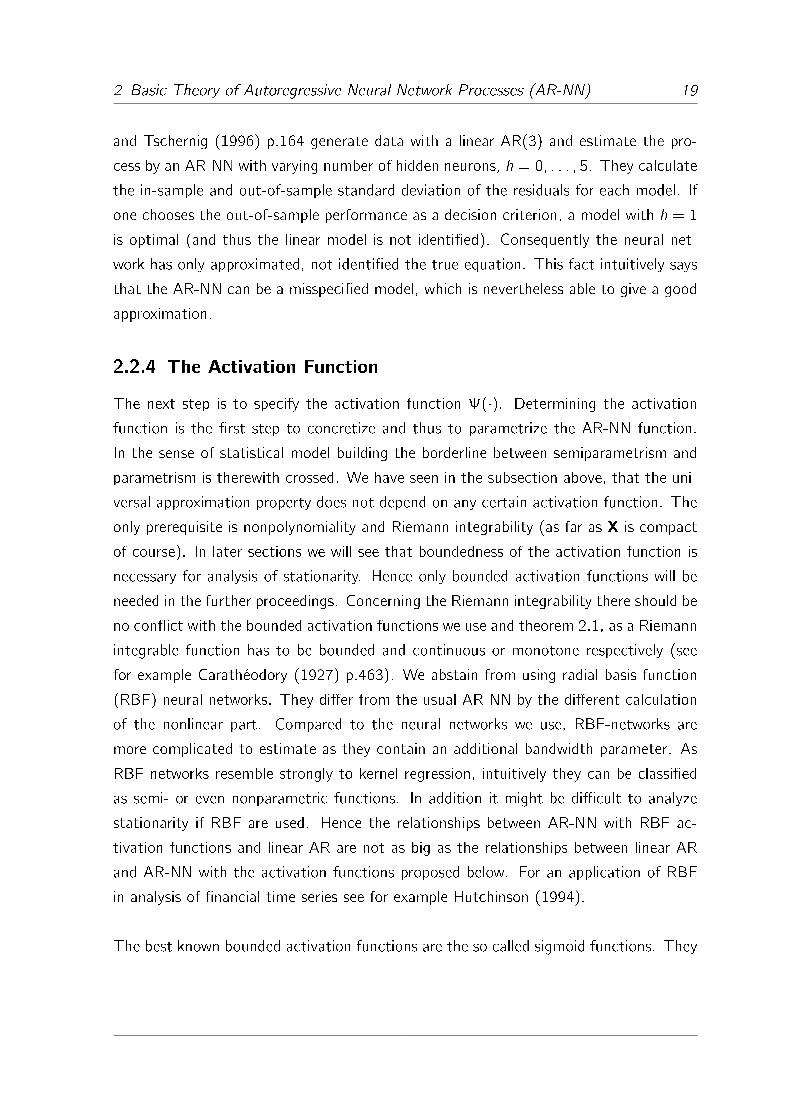
In �gure 2.4 a linear series of 501 observations (T = 501) equally distributed on the
intervals (a) [�1; 1] and (b) [�10; 10] is transformed by the mentioned bounded acti-
vation functions to visualize their behavior concerning the input range. It is observable
that the larger the input is, the stronger the activation functions reacts. Note that the
size of the input is not only determined by the input neurons but also by the weights.
Only those bounded functions which are used as activation functions for neural networks
in literature are described in this section. Thus, this section does not claim to be a per-
fect list of all possible bounded activation functions. However it should be mentioned
here that the universal approximation property does not depend on the speci�c form of
the activation function.
A sigmoid activation function can be interpreted as a smooth transition function, which
is especially able to handle structural breaks. A closely related method to AR-NN's with
sigmoid activation function is the smooth transition autoregression model (STAR). A
simple version of a STAR(1) is (similar to Granger and Teräsvirta (1993) p.39):
xt = �0 + �1xt�1 +( 0 + 1xt�1)�(xt�1) + "t ; (2.2.18)
whereas(�) is for example the tanh. This equation can be interpreted as a linear AR(1)
with a structural break in the regression coe�cient. The transition from regression
coe�cient �1 to �1 + � proceeds "smoothly" along the tanh function (an alternative
would be a threshold function, which directly shifts from one model to the other). An
AR-NN(1) with h = 1,
xt = �0 + �1xt�1 +( 0 + 1xt�1)� + "t ; (2.2.19)
can be interpreted as a STAR with structural break in the constant. Nevertheless
equation (2.2.18) can be approximated by an AR-NN(1) with su�cient hidden neurons,
as the e�ect of �(xt�1) in (2.2.18) can be approximated by the combination of several
constants. To illustrate this we consider a simple model of an AR(1) with structural
break in the regression coe�cient as shown in �gure 2.5. In this case - for simpli�cation

2 Basic Theory of Autoregressive Neural Network Processes (AR-NN) 24
- (�) is a threshold function. This graph shows the following transition autoregression
(TAR) process:
xt = �0 + �1xt�1 +( 1xt�1)�(xt�1 � 2) (2.2.20)
with
(x) =
1 if x � 1
0 if x < 1(2.2.21)
and �0 = 1, �1 = 0:5, 1 = 0:5 and � = 0:5. Now we consider an AR-NN(1) with 2
hidden neurons and function (2.2.21) as activation function:
xt = �0 + �1xt�1 +( 1xt�1)�1 +( 2xt�1)�2 (2.2.22)
with �0 = 1, �1 = 0:5, 1 =13, �1 = 1, 2 =
15and �2 = 1. Figure 2.6 shows how the
AR-NN(1) in equation (2.2.22) approximates the TAR(1) of equation (2.2.20). If the
number of hidden neurons is increased, the approximation becomes more accurate. To
demonstrate this, we use 4 hidden neurons such that the AR-NN(1) equation becomes
xt = �0 + �1xt�1 +
4∑i=1
( ixt�1)�i (2.2.23)
with �0 = 1, �1 = 0:5, 1 = 12, 2 = 1
3, 3 = 1
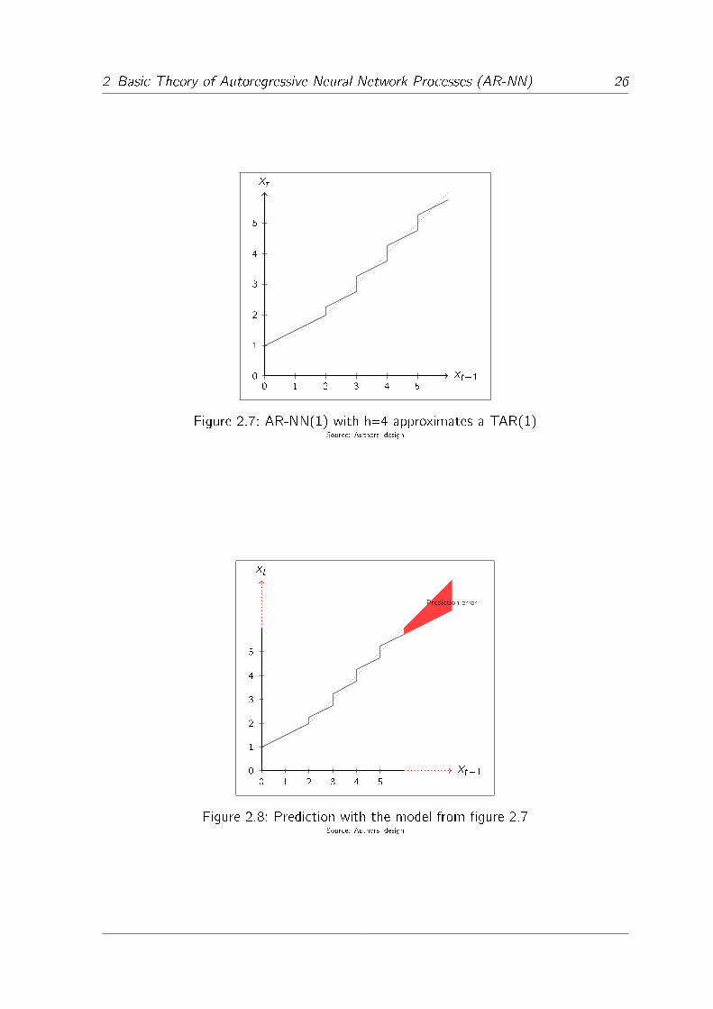
4, 4 = 1
5, �1 = 0:25, �2 = 0:5,
�3 = 0:5 and �4 = 0:5. The result is shown in �gure 2.7. A structural break in the
regression coe�cient can be approximated by a su�ciently large number of structural
breaks in the constant (which are represented by the hidden neurons in an AR-NN).
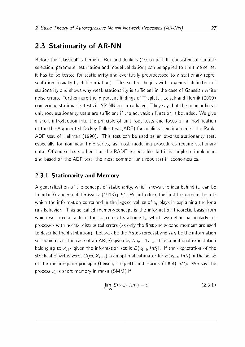
This simple example shows the advantage of AR-NN: The number of hidden neurons
can be increased until an optimal approximation is reached. Concerning prediction, the
AR-NN only delivers appropriate results in the short run. Consider �gure 2.8: The
larger the prediction horizon becomes, the more the original and the estimated series
diverge and the more the prediction error increases. Our empirical results also con�rm
the �nding that AR-NN perform well mainly in one and two step predictions: For higher
step predictions they are dominated by their linear part.
In the further proceedings we will use often the tanh activation function for the follow-
ing two reasons: Firstly, it is one of the most common activation functions in literature,
and secondly, its derivations can be calculated relatively easily and thus it is easy to
handle.

2 Basic Theory of Autoregressive Neural Network Processes (AR-NN) 25
xt�1
xt
0 1 2 3 4 50
1
2
3
4
5
Figure 2.5: AR(1) with structural breakSource: Authors' design
xt�1
xt
0 1 2 3 4 50
1
2
3
4
5
Figure 2.6: AR-NN(1) with h=2 approximates a TAR(1)Source: Authors' design
2 Basic Theory of Autoregressive Neural Network Processes (AR-NN) 26
xt�1
xt
0 1 2 3 4 50
1
2
3
4
5
Figure 2.7: AR-NN(1) with h=4 approximates a TAR(1)Source: Authors' design
xt�1
xt
0 1 2 3 4 50
1
2
3
4
5
Prediction error
Figure 2.8: Prediction with the model from �gure 2.7Source: Authors' design
2 Basic Theory of Autoregressive Neural Network Processes (AR-NN) 27
2.3 Stationarity of AR-NN
Before the �classical� scheme of Box and Jenkins (1976) part II (consisting of variable
selection, parameter estimation and model validation) can be applied to the time series,
it has to be tested for stationarity and eventually preprocessed to a stationary repre-
sentation (usually by di�erentiation). This section begins with a general de�nition of
stationarity and shows why weak stationarity is su�cient in the case of Gaussian white
noise errors. Furthermore the important �ndings of Trapletti, Leisch and Hornik (2000)
concerning stationarity tests in AR-NN are introduced. They say that the popular linear
unit root stationarity tests are su�cient if the activation function is bounded. We give
a short introduction into the principle of unit root tests and focus on a modi�cation
of the the Augmented-Dickey-Fuller test (ADF) for nonlinear environments, the Rank-
ADF test of Hallman (1990). This test can be used as an ex-ante stationarity test,
especially for nonlinear time series, as most modelling procedures require stationary
data. Of course tests other than the RADF are possible, but it is simple to implement
and based on the ADF test, the most common unit root test in econometrics.
2.3.1 Stationarity and Memory
A generalization of the concept of stationarity, which shows the idea behind it, can be
found in Granger and Teräsvirta (1993) p.51. We introduce this �rst to examine the role
which the information contained in the lagged values of xt plays in explaining the long
run behavior. This so called memory-concept is the information theoretic basis from
which we later attach to the concept of stationarity, which we de�ne particularly for
processes with normal distributed errors (as only the �rst and second moment are used
to describe the distribution). Let xt+h be the h step forecast and Inft be the information
set, which is in the case of an AR(n) given by Inft : Xt�1. The conditional expectation
belonging to xt+h given the information set is E(xt+hjInft). If the expectation of the
stochastic part is zero, G(�; Xt�1) is an optimal estimator for E(xt+hjInft) in the senseof the mean square principle (Leisch, Trapletti and Hornik (1998) p.2). We say the
process xt is short memory in mean (SMM) if
limh!1
E(xt+hjInft) = c (2.3.1)
2 Basic Theory of Autoregressive Neural Network Processes (AR-NN) 28
and the distribution of the random variable c does not depend on Inft . In the special
case of mean-stationarity as we will see in de�nition 2.2, a constant mean is a special
case of SMM. In contrast, if the distribution of c depends on Inft , the process xt is
called long memory in mean (LMM).
We now consider the conditional distribution of the h step forecast expressed by the
probability P rob(xt+h � x jInft). If the limit of this conditional distribution,
limh!1
P rob(xt+h � x jInft) (2.3.2)
does not depend on Inft , the process xt is said to be short memory in distribution
(SMD). Just another notation for this would be if for all sets C1 and C2 holds
jP rob(xt+h 2 C1jInft 2 C2)� P rob(xt+h 2 C1)j ���!h!1
0 (2.3.3)
If in contrast (2.3.2) depends on Inft , the process is called long memory in distribution
(LMD). In the case of a stationary AR(n) the distribution of the process is determined
by "t which is by de�nition 2.1 i.i.d. N(0; �2) with constant �2. Thus a stationary
process is SMD. The property SMD implies also the property SMM but Granger and
Teräsvirta (1993) pp.51-52 provide some examples that this relation does not work in
the other direction.
Stronger than the term SMD would be the term stationary in distribution, which means
that (2.3.2) is constant. According to Leisch, Trapletti and Hornik (1998) p.2 this
also can be called strict stationarity as it incudes of course stationarity in mean. The
term weak stationarity as we will de�ne it in the following, according to Schlittgen
and Streitberg (1995) p.100 and Hamilton (1994) p.45, is included in the de�nition of
strict stationarity. Weak stationary means that only the �rst and second moment have
to be stationary. Particularly for normal distributed processes weakly stationarity can
be used synonymously for strict stationarity as the distribution is mainly characterized
by the �rst and second moment (this is intuitively clear if one considers the Gaussian
probability density function).
2 Basic Theory of Autoregressive Neural Network Processes (AR-NN) 29
De�nition 2.2 (Stationarity):
A stochastic process xt is called
� Mean-Stationary if E(xt)=constant 8 t 2 T
� Variance-Stationary if �2t=�
2=constant 8 t 2 T
� Covariance-Stationary if cov(xt�i ; xt�j) = constant 8 t 2 T and i ; j = 0; : : : ; n
� Weakly Stationary if it is mean-stationary and covariance-stationary
Remark 2.2.1:
If a process is covariance-stationary the covariance of any two lag variables depends only
on the distance between the lags. Clearly the i.i.d. N(0; �2) process "t is stationary as
E("t) = 0 8t, �2t=�
2 8t and
cov(xt�i ; xt�j) =
0 i f i 6= j
�2 i f i = j: (2.3.4)
Remark 2.2.2:
Covariance stationarity implies variance stationarity as cov(xt�i ; xt�i)=
cov(xt�j ; xt�j) = �2.
2.3.2 Markov Chain Representation and the Invariance Measure
For the further procedure we need a function representing equation (2.2.8) which maps
from Rn ! Rn. We get it by the Markov chain representation
Xt = H(Xt�1) + Et : (2.3.5)
The vectors belonging to this equation are Xt=(xt ; xt�1; : : : ; xt�n+1)>, H(Xt�1) =
(G(�; Xt�1); xt�1; : : : ; xt�n+1)> and Et = ("t ; 0; : : : ; 0)
> (see Trapletti, Leisch and
Hornik (2000) p.2429). A Markov chain resembles a multivariate AR(1). Markov chain
theory provides some additional measures to analyze the stability (for a detailed in-
troduction see Haigh (2010) pp.88-89). Our aim is to use those stability measures
for formulating a theorem concerning the stability of AR-NN (theorem 2.2). Equation

2 Basic Theory of Autoregressive Neural Network Processes (AR-NN) 30
(2.3.5) provides the link between the measures from Markov chain theory and AR-
NN(n) with n > 1.
Again we need the term SMD. As we have seen that SMD includes SMM, a Markov chain
which is SMD is also stationary (see Resnick (1992) p.116). To show under which condi-
tions a Markov chain like equation (2.3.5) is strictly stationary (and thus weakly station-
ary in the case of Gaussian WN errors) we need a term for the probability that xt moves
from point x to a set A in k steps, denoted by P robk(x;A)= P rob(xt+k 2 Ajxt = x).
This probability is called the k-step transition probability (Fonseca and Tweedie (2002)
p.651). If this transition probability is constant for all steps k we have in fact a strictly
stationary process. Account for the fact that the Markov chain (2.3.5) is a AR(1), then
the transition probability is equal to the �rst probability term in (2.3.3). Let jj � jj bethe total deviation norm. If a constant probability measure dependent on the selection
of A, �(A), exists such that
limk!1
�k jjP robk(x;A)� �(A)jj = 0; (2.3.6)
the process is called geometrical ergodic and ergodic for the special case � = 1. The
probability measure has to satisfy the invariance equation
�(A) =∫
Rn
P rob(x;A)�dx: (2.3.7)
� is also called the stationary or invariant measure. Geometrical ergodicity implies sta-
tionarity as the distribution converges to �, which is constant. Thus a geometrical
ergodic process is asymptotic stationary (because of the convergence). If a process
already starts with �, it is strictly stationary. In addition we need the properties irre-
ducible and aperiodic. Irreducible can be explained informally as the property that any
point of the state space of the process can be reached independently from the starting
point. The process is aperiodic, if it is not possible that the process returns to certain
sets only at certain time points. If the errors in our process are i.i.d. N(0; �2), it is
certainly irreducible and aperiodic (see Trapletti, Leisch and Hornik (2000) p.2431).
Hence we will not further discuss those terms as they are included in the Gaussian WN
assumption on the errors.
2 Basic Theory of Autoregressive Neural Network Processes (AR-NN) 31
2.3.3 Unit Roots and Stationarity of AR-NN
This section is mainly based on Trapletti, Leisch and Hornik (2000) p.2431. For the
further proceeding we �rst introduce some notations from linear time series analysis:
The unit roots (UR) of the characteristic polynomial. Consider the scalar linear AR(n)
xt = �1xt�1 + �t�2 + : : :+ �nxt�n + "t (2.3.8)
"t = xt � �1xt�1 � �t�2 � : : :� �nxt�n (2.3.9)
The characteristic polynomial of this process is denoted by
1� �1z2 � �2z
2 � : : : �nz2 = 0; (2.3.10)
see Schlittgen and Streitberg (1995) p.100. The solutions z of this equation are called
roots. The process is weakly stationary if the roots are outside the unit circle and thus
jz j > 1 and explosive or chaotic if jz j < 1, (Hatanaka (1996) p.22). A condition equiv-
alent to the condition that the roots should be outside the unit circle is j�i j < 1 (see
Schlittgen and Streitberg (1995) pp.123-124 and Hatanaka (1996) pp.22-23).
If the process has its roots outside the unit circle, it can be inverted to an in�nite
MA representation based on the residuals. In this case it can easily be shown that xt is
stationary, because it only depends on the white-noise process "t . Therefore we rewrite
equation (2.3.8) using the lag-operator L:
xt = �(L)xt + "t = (1� �1L� : : :� �nLn)xt + "t : (2.3.11)
The process has an in�nite MA representation if the inverse �lter ��1(L) exists. There-
with equation (2.3.11) becomes
xt = ��1(L)"t =
1∑i=1
�i"t�i : (2.3.12)
The inverse �lter exists only if jz j < 1, see Schlittgen and Streitberg (1995) p.122 and
Hassler (2007) p.48.
2 Basic Theory of Autoregressive Neural Network Processes (AR-NN) 32
In the border case the largest solution is jz j = 1. Equation (2.3.10) becomes
1 = �1 + �2 + : : :+ �n: (2.3.13)
We say the process has a unit root. This process can be stationarized by di�erentiation,
because the stable �lter (1 � L) can be splitted o� from �(L). Without stationariza-
tion via di�erences the process has no MA(1) representation and is not stationary. A
nonstationary process with one UR is called process of integration order 1. An impor-
tant theorem concerning the stationarity of an AR-NN can be formulated according to
Trapletti, Leisch and Hornik (2000) pp. 2430-2431:
Theorem 2.2 (Trapletti, Leisch and Hornik (2000) pp. 2430-2431 theorem 1):
Assume that "t is a Gaussian WN process and is bounded. The characteristic poly-
nomial of the linear part (the direct edges between input and output nodes without the
bias) is denoted as
�(z) = 1�n∑i=1
�izi : (2.3.14)
The condition
�(z) 6= 0 8z; jz j � 1; (2.3.15)
is su�cient but not necessary that the process xt is geometrical ergodic and asymptotic
stationary. If Ej"t j2 <1, the process is weakly stationary.
PROOF: The proof can be formulated in two di�erent ways using two previous �ndings:
The �rst proof in Trapletti, Leisch and Hornik (2000) p. 2438 uses the results of Tjø-
stheim (1990) and Meyn and Tweedie (1993). The alternative, the proof of theorem
1 (Leisch, Trapletti and Hornik (1998) p.4) in Leisch, Trapletti and Hornik (1998) pp.
9-10 uses the results of Chan and Tong (1985).
The bias is is processed like a constant and is thus not part of the characteristic polyno-
mial (like deterministic drifts in linear AR(n)). We see that stationarity of the process
depends on the linear part and we can use the usual unit root theory from linear time
series analysis to test for stationarity. If we have no linear part, the AR-NN always leads
to a stationary representation (because of the boundedness of the activation function),
2 Basic Theory of Autoregressive Neural Network Processes (AR-NN) 33
see Trapletti, Leisch and Hornik (2000) p.4.
Next it has to be shortly explained why (weak) stationarity of the linear part is not
a necessary condition. If one root is on the unit circle, we expect Random Walk behav-
ior of the process with or without time trend (drift). But it is possible that the nonlinear
part of the process causes a drift towards a stationary solution. This is meant by the
statement that stationarity of the linear part is su�cient but not necessary in theo-
rem 2.2. For further details see Trapletti, Leisch and Hornik (2000) p.2432. Theorem
2.2 outlines also the hybrid character (composed of a linear and a nonlinear part) of
AR-NN as we use them. Practical application especially with unscaled data shows that
the squashing property for bounded activation functions tends to produce stationary
outputs.
2.3.4 The Rank Augmented Dickey-Fuller Test
In this subsection we consider a procedure based on the ADF test. This test is most
common in econometrics to analyze the UR of a given time series (originally developed
by Dickey and Fuller (1979) for linear AR(1)). Dickey-Fuller tests for higher order linear
AR are called ADF tests, see Schlittgen and Streitberg (1995) p.300. In the following
we give a short overview over the test and consider some problems using UR tests.
At �rst the linear AR with unknown order n of equation (2.1.2) is rearranged:
xt = a1xt�1 + a2�xt�1 + a3�xt�2 + : : : an�xt�n + "t (2.3.16)
whereas a1 = �1 + �2 + : : : �n, a2 = ��2 � : : :� �n, a3 = ��3 � : : :� �n, an = ��n
and "t are the residuals of the equation. The null hypothesis "H0 : a1 = 1" implies that
the process is integrated of order one which means it can be stationarized by applying
�rst di�erences. The alternative is "H1 : a1 < 1", which means that the process is
already stationary. Usually the following test statistic is applied:
TADF =a1 � 1√
�2"t�∑T
t=2 x2t�1
: (2.3.17)
�2"t
(the variance of the residuals) and a1 are received by linear regression applied at
equation (2.3.16), see Schlittgen and Streitberg (1995) p.300. The distribution of TADF
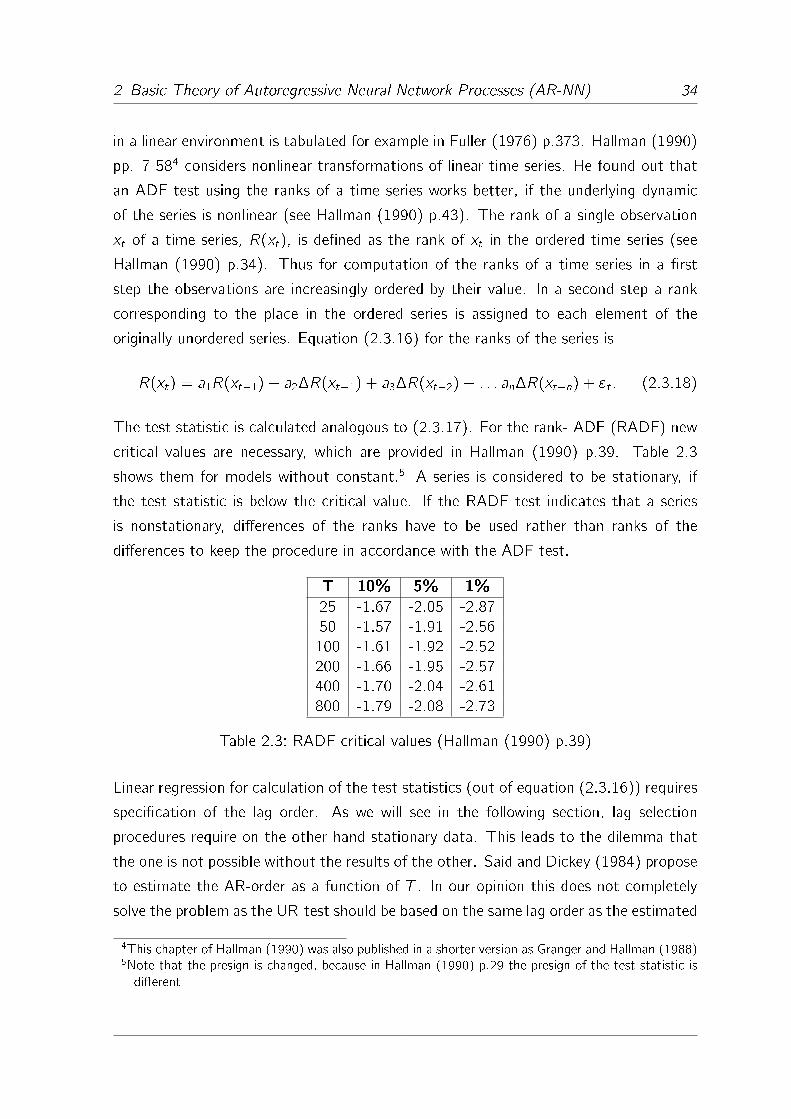
2 Basic Theory of Autoregressive Neural Network Processes (AR-NN) 34
in a linear environment is tabulated for example in Fuller (1976) p.373. Hallman (1990)
pp. 7-584 considers nonlinear transformations of linear time series. He found out that
an ADF test using the ranks of a time series works better, if the underlying dynamic
of the series is nonlinear (see Hallman (1990) p.43). The rank of a single observation
xt of a time series, R(xt), is de�ned as the rank of xt in the ordered time series (see
Hallman (1990) p.34). Thus for computation of the ranks of a time series in a �rst
step the observations are increasingly ordered by their value. In a second step a rank
corresponding to the place in the ordered series is assigned to each element of the
originally unordered series. Equation (2.3.16) for the ranks of the series is
R(xt) = a1R(xt�1) + a2�R(xt�1) + a3�R(xt�2) + : : : an�R(xt�n) + "t : (2.3.18)
The test statistic is calculated analogous to (2.3.17). For the rank- ADF (RADF) new
critical values are necessary, which are provided in Hallman (1990) p.39. Table 2.3
shows them for models without constant.5 A series is considered to be stationary, if
the test statistic is below the critical value. If the RADF test indicates that a series
is nonstationary, di�erences of the ranks have to be used rather than ranks of the
di�erences to keep the procedure in accordance with the ADF test.
T 10% 5% 1%
25 -1.67 -2.05 -2.87
50 -1.57 -1.91 -2.56
100 -1.61 -1.92 -2.52
200 -1.66 -1.95 -2.57
400 -1.70 -2.04 -2.61
800 -1.79 -2.08 -2.73
Table 2.3: RADF critical values (Hallman (1990) p.39)
Linear regression for calculation of the test statistics (out of equation (2.3.16)) requires
speci�cation of the lag order. As we will see in the following section, lag selection
procedures require on the other hand stationary data. This leads to the dilemma that
the one is not possible without the results of the other. Said and Dickey (1984) propose
to estimate the AR-order as a function of T . In our opinion this does not completely
solve the problem as the UR-test should be based on the same lag order as the estimated
4This chapter of Hallman (1990) was also published in a shorter version as Granger and Hallman (1988)5Note that the presign is changed, because in Hallman (1990) p.29 the presign of the test statistic is
di�erent

2 Basic Theory of Autoregressive Neural Network Processes (AR-NN) 35
model. Therefore a good strategy might be to de�ne a maximal lag order m at �rst and
then calculate the RADF test statistic for all lags from 1 to m. The maximal lag order
should account for the fact that a realistic relation between n and T is kept. In Said and
Dickey (1984) p.600 the optimal relation between lags and observations is determined
by 3pT �m ! 0 for example. Another possibility is to prespecify the number of hidden
neurons and to determine a maximal lag order which accounts for the fact that the
relation between parameters and observations should be 1=10. For example if we have
h = 2 hidden neurons, the maximal number of lags should be m � 1=30T+5=3. Usually
we expect to �nd for each lag order n = 1; : : : ; m that the process is nonstationary and
can be stationarized by the �rst di�erences. Subsequently one of the several variable
selection procedures from the following section can be applied to the stationarized data
to �nd the optimal lag order n for the models.
3 Modelling Univariate AR-NN 36
3 Modelling Univariate AR-NN
In this chapter we show how one belongs to an univariate AR-NN model for a given time
series. Only estimating the parameters is certainly not su�cient to receive an appropri-
ate model. We follow Box and Jenkins (1976) part II, who propose to proceed in three
steps: Variable selection, parameter estimation and model validation (parameter tests).
Before we can start with the �rst step, it has to be assured that the data are stationary.
If they are nonstationary, stationarization as an additional transformation is neces-
sary. The aim of doing so is to avoid the problem of spurious regression mentioned by
Granger and Newbold (1974), which may occur if regression of any nonstationary time
series which are in reality uncorrelated on each other indicates signi�cantly correlated
results. Although this problem is analyzed only for linear time series, several authors
state that it is relevant for neural networks too (Lee, White and Granger (1993) p.287,
Anders (1997) p.99, Trapletti, Leisch and Hornik (2000) p.2440). Steurer (1996)
p.120-124 shows by empirical investigation that neural networks only work accurate for
stationary data. Hence the methods presented below are only applicable at stationary
time series. For testing procedures for stationarity we refer to section 2.3.4.
Nonlinearity tests are an addition to the common framework of time series modelling.
Testing a time series on hidden nonlinearity before an AR-NN model is adjusted is nec-
essary for two reasons: Firstly the additional e�ort necessary for a nonlinear model
compared to a linear one has to be justi�ed. Secondly as we know from section 2.2.3
an AR-NN model performs equal to a linear model if the investigated time series is
determined by a linear process. If one accounts for the additional e�ort necessary for
the nonsigni�cant linear part in such a case, the AR-NN is inferior than a simple linear
AR.
In �gure 3.1 a �ow chart shows the steps to build an AR-NN model for a given time
series. This �gure may serve as a general plan to construct an AR-NN model of any
given time series as also the �augmented� philosophy is included (increasing the number
of hidden neurons step by step, starting with h=1). The �gure also serves as a guideline
for the sections of this chapter.

3 Modelling Univariate AR-NN 37
Figure 3.1: Flow chart AR-NN model buildingSource: Authors' design, based on the �gures in Anders (1997) p.37 and pp.127-132

3 Modelling Univariate AR-NN 38
3.1 The Nonlinearity Test
In the previous sections we have become acquainted with the structure of AR-NN.
Compared to a simple linear model it is much more complicated. If a series is linear,
the additional e�ort is of no use. To avoid this, the series should be tested on hidden
nonlinearity at the �rst. The nonlinearity test of Teräsvirta, Lin and Granger (1993),
described in this section, is a simple and e�cient method, based on previous results of
White (1989a). The basic idea is to approximate the AR-NN by a Taylor polynomial.
Such an approximation is necessary, because the distribution of the parameters of the
AR-NN does not always exist (only if the conditions in section 3.4.2.1 are achieved).
In contrast the distribution of the parameters of the Taylor polynomial always exists.
An existing distribution of the parameters is a prerequisite for parameter tests like the
Lagrange-multiplier test. As we have not yet speci�ed the number of lags, the test
on hidden nonlinearity should be executed on all lags from 1 to a prespeci�ed maximal
number of lags. Empirical application shows, that a time series may be nonlinear for
one lag order as well as linear for other lag orders.
3.1.1 Taylor Expansion
Taylor expansion is a method to approximate nonlinear functions by a chain of polyno-
mials of increasing order. The concept is easy to understand, hence this approximation
method will be of use several times in this dissertation. Its two main advantages are
its general approximation property and the existence of a distribution of its parameters
and therefore its adaptability for parameter tests. We specify it in the following:
Based on Weierstrass (1885) and extended by Stone (1948), the Stone-Weierstrass
theorem says that a Taylor polynomial of su�cient high order can approximate any
function (see Medeiros, Teräsvirta and Rech (2006) pp.52-53). Taylor expansion of
order k for a function F (x) around a point x0 is given by
F (x) = F (x0) +F 0(x0)1!
(x � x0) +F 00(x0)2!
(x � x0)2 + : : :+
F k(x0)
k!(x � x0)
k ; (3.1.1)
with F 0(x0) as the �rst derivative of F (x0) respective x0, F00(x0) the second derivative
and F k(x0) the kth derivative, see Anders (1997) p.52. If x0 = 0 (Taylor expansion
around 0) the series (3.1.1) is also called Maclaurin series. If our aim is to approximate
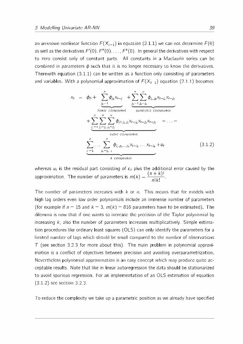
3 Modelling Univariate AR-NN 39
an unknown nonlinear function F (Xt�1) in equation (2.1.1) we can not determine F (0)
as well as the derivatives F 0(0); F 00(0); : : : ; F k(0). In general the derivatives with respect
to zero consist only of constant parts. All constants in a Maclaurin series can be
combined in parameters � such that it is no longer necessary to know the derivatives.
Therewith equation (3.1.1) can be written as a function only consisting of parameters
and variables. With a polynomial approximation of F (Xt�1) equation (2.1.1) becomes
xt = �0 +
n∑j1=1
�j1xt�j︸ ︷︷ ︸l inear component
+
n∑j1=1
n∑j2=j1
�j1;j2xt�j1xt�j2︸ ︷︷ ︸quadratic component
+
n∑j1=1
n∑j2=j1
n∑j3=j2
�j1;j2;j3xt�j1xt�j2xt�j3︸ ︷︷ ︸cubic component
+ : : :+
n∑j1=1
: : :
n∑jk=jk�1
�j1;j2;:::;jkxt�j1 : : : xt�jk︸ ︷︷ ︸k component
+ut (3.1.2)
whereas ut is the residual part consisting of "t plus the additional error caused by the
approximation. The number of parameters is m(k) =(n + k)!
n!k!.
The number of parameters increases with k or n. This means that for models with
high lag orders even low order polynomials include an immense number of parameters
(for example if n = 15 and k = 3, m(k) = 816 parameters have to be estimated). The
dilemma is now that if one wants to increase the precision of the Taylor polynomial by
increasing k , also the number of parameters increases multiplicatively. Simple estima-
tion procedures like ordinary least squares (OLS) can only identify the parameters for a
limited number of lags which should be small compared to the number of observations
T (see section 3.2.3 for more about this). The main problem in polynomial approxi-
mation is a con�ict of objectives between precision and avoiding overparametrization.
Nevertheless polynomial approximation is an easy concept which may produce quite ac-
ceptable results. Note that like in linear autoregression the data should be stationarized
to avoid spurious regression. For an implementation of an OLS estimation of equation
(3.1.2) see section 3.2.3.
To reduce the complexity we take up a parametric position as we already have speci�ed
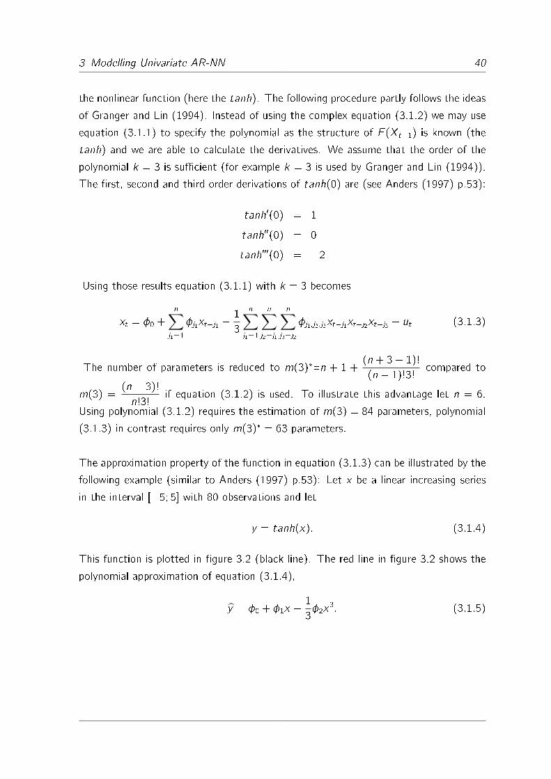
3 Modelling Univariate AR-NN 40
the nonlinear function (here the tanh). The following procedure partly follows the ideas
of Granger and Lin (1994). Instead of using the complex equation (3.1.2) we may use
equation (3.1.1) to specify the polynomial as the structure of F (Xt�1) is known (the
tanh) and we are able to calculate the derivatives. We assume that the order of the
polynomial k = 3 is su�cient (for example k = 3 is used by Granger and Lin (1994)).
The �rst, second and third order derivations of tanh(0) are (see Anders (1997) p.53):
tanh0(0) = 1
tanh00(0) = 0
tanh000(0) = �2
Using those results equation (3.1.1) with k = 3 becomes
xt = �0 +
n∑j1=1
�j1xt�j1 �1
3
n∑j1=1
n∑j2=j1
n∑j3=j2
�j1;j2;j3xt�j1xt�j2xt�j3 + ut (3.1.3)
The number of parameters is reduced to m(3)�=n + 1 +(n + 3� 1)!
(n � 1)!3!compared to
m(3) =(n + 3)!
n!3!if equation (3.1.2) is used. To illustrate this advantage let n = 6.
Using polynomial (3.1.2) requires the estimation of m(3) = 84 parameters, polynomial
(3.1.3) in contrast requires only m(3)� = 63 parameters.
The approximation property of the function in equation (3.1.3) can be illustrated by the
following example (similar to Anders (1997) p.53): Let x be a linear increasing series
in the interval [�5; 5] with 80 observations and let
y = tanh(x): (3.1.4)
This function is plotted in �gure 3.2 (black line). The red line in �gure 3.2 shows the
polynomial approximation of equation (3.1.4),
y = �0 + �1x � 1
3�2x
3: (3.1.5)
3 Modelling Univariate AR-NN 41
This equation can be estimated by an OLS procedure. We see that the polynomial is
able to approximate the original tanh quite well, but the regression in the "transition"
part is more �at.1
0 20 40 60 80
-1.0
-0.5
0.0
0.5
1.0
x
yPolynomialtanh
Figure 3.2: Taylor polynomial approximation of the tanhSource: Authors' design, based on Anders (1997) p.53 �gure 3.5
3.1.2 The Lagrange-Multiplier Tests
The test of Teräsvirta, Lin and Granger (1993) is an advancement of the test of
White (1989a). Both tests are executed as Lagrange-multiplier (LM) tests. The main
di�erence is, that in the test of White (1989a) weights for the additional hidden neurons
are determined randomly, whereas in the test of Teräsvirta, Lin and Granger (1993) the
nonlinear part is approximated by Taylor expansion. The main di�culty with the test
of White (1989a) is the problem of inconsistency in the case of heteroscedasticity in
calculation of the test statistic. Another problem is the arbitrariness in selection of
the nonlinear hidden units weights. As the test of Teräsvirta, Lin and Granger (1993)
tries to overcome those problems, we use it in the further procedure. The following
description starts with the test of White (1989a) (see also Anders (1997) pp.69-72) in
subsection 3.1.2.1 to introduce the basic principles of LM nonlinearity tests. Subsection
3.1.2.2 continues with the advancements of Teräsvirta, Lin and Granger (1993) (see
also Anders (1997) pp.67-69)
1The main di�erence between our �gure 3.2 and the �gure in Anders (1997) p.53 are the parameters;
In our example they are estimated by OLS, in Anders (1997) p.53 they are set 1. The advantage of
our result is, that the polynomial estimator is bounded on the right and left end of the "transition"
part. However the approximation of the boundaries is not appropriate as they are not �at in the
polynomial.
3 Modelling Univariate AR-NN 42
3.1.2.1 The Test of White
Neglected nonlinearity in the sense of White (1989a) p.45 means, that there is some
nonlinearity which is not covered by the linear AR in the process. If neglected nonlinearity
exists - and the process is in fact determined by a nonlinear function - the linear AR model
is misspeci�ed. Now the test should examine whether the linear model is misspeci�ed
or not. Thus the null hypothesis in the test is, that an estimated linear model
xt = �0 + �1xt�1 + : : :+ �nxt�n + "t = �0 + A>Xt�1 + "t (3.1.6)
with Xt�1 = (xt�1; : : : ; xt�n)> and A = (�1; : : : ; �n)> is able to explain the "true"
function F (Xt�1) in equation (2.1.1). The hypothesis formally can be written as
H0 : P rob(F (Xt�1) = �0 + A>Xt�1
)= 1 (3.1.7)
The alternative hypothesis is, that the linear AR does not explain F (Xt�1),
H1 : P rob(F (Xt�1) = �0 + A>Xt�1
)< 1: (3.1.8)
The test of H0 against H1 is constructed on the basis of the WN assumption on the
residuals. If H0 does not apply and not the whole true function F (Xt�1) is explained by
�0 + A>Xt�1, then some neglected nonlinearity is spuriously contained in the stochas-
tic part. Consider equation (3.1.6). To separate the neglected nonlinearity from the
stochastic part we must rewrite this equation as
xt = �0 + A>Xt�1 + ut ; (3.1.9)
with
ut =(F (Xt�1)� �0 � A>Xt�1
)+ "t (3.1.10)
and "t is i.i.d. with N(0; �2). The �rst term of equation (3.1.10) notes the part of
F (Xt�1) which is not covered by the linear process, the neglected nonlinearity. If such
is present, the residuals ut are actually not equal to the stochastic part "t but contain
the neglected nonlinearity in addition. If H0 applies, the �rst term of equation (3.1.10)
vanishes and the residual term ut consists only of the Gaussian distributed WN part "t .
In this case equation (3.1.9) becomes (3.1.6) and the linear estimation is appropriate.

3 Modelling Univariate AR-NN 43
If H0 is true, there is no correlation between the residual term and Xt�1, which means
that the conditional expectation E(ut jXt�1) = E("t jXt�1) = 0 (see also section 2.1.1).
Hence even if Xt�1 is transformed by any function H(Xt�1), the residual term ut is not
correlated with that transformation, because
E(H(Xt�1) � ut) = E(E(H(Xt�1) � ut jXt�1)) = E(H(Xt�1))E(ut jXt�1) = 0: (3.1.11)
We de�ne H(Xt�1) as an additional hidden unit, called �phantom unit�. It can be con-
structed using the activation function of the network , random weights 0; 1; : : : ; n
and a random �. Note that in the original paper of White (1989a) more than one
additional hidden unit can be used. To keep the test manageable, we propose to use
only one additional unit, also in regard of a proper relation between observations T and
the number of parameters. The following hypotheses are based on the AR-NN equation
xt = �0 + A>Xt�1 +( 0 + �>Xt�1)� + "t ; (3.1.12)
which corresponds to equation 2.2.7 with h=1. The test of White (1989a) is based only
on the -weights. Respecting this, a consequence of the null hypothesis H0 (3.1.7) is
H�0 : E
(( 0 + �>Xt�1
) � ut j i) = 0 8 i = 0; : : : ; n (3.1.13)
with the alternative
H�1 : E
(( 0 + �>Xt�1
) � ut j i) 6= 0 8 i = 0; : : : ; n (3.1.14)
Thus the rejection of H�0 means rejecting H0. However not rejecting H
�0 does not mean
not rejecting H0. Consequently testing H�0 against H�
1 is not consistent for testing H0
against H1. But as a test of H�0 against H�
1 can be implemented as a LM test, we
continue with that procedure.
In order to get to the test statistic �rst the expectation E(( 0 + �>Xt�1
) � ut j i) hasto be estimated, which is done by calculating the average:
E(( 0 + �>Xt�1
) � ut j i) = 1
T
T∑t=1
(( 0 + �>Xt�1
) � ut) (3.1.15)
3 Modelling Univariate AR-NN 44
If the null hypothesis is not rejected, the value of (3.1.15) should be around zero
(White (1988) p.453). If in contrast the null hypothesis is rejected, the value of
(3.1.15) is away from zero. Vice versa one can test if the expectation is signi�-
cantly away from zero to decide if H�0 should be rejected. Therefore the distribution
of 1pT
∑T
t=1
(( 0 + �>Xt�1
) � ut) should be known. According to the central limit
theorem it converges to N(0; �2�), a normal distribution with zero mean and variance
�2� (denotes here the variance of the additional hidden neuron) as T !1.2 The test
statistic
T1 =1pT
T∑t=1
(( 0 + �>Xt�1
) � ut) � 1
�2� �1pT
T∑t=1
(( 1 + �>Xt�1
) � ut) (3.1.16)
is �2 distributed with one degree of freedom. The test is implemented as �2-test, which
means that H�0 is rejected if it exceeds a certain percentile of the (above) �
2-distribution.
However sometimes it might be sometimes di�cult to determine �2�. Therefore the
parameter estimators have to be consistent, which is only given under certain condi-
tions (see section 3.4.2.1). Hence a procedure is used, which leads to test statistics
asymptotically equivalent to 3.1.16:
First an arti�cial linear regression is performed:
ut = �1r(�0 + A>Xt�1
)+�2
(( 0 + �>Xt�1
))+ u�t ; (3.1.17)
whereas �1 and �2 are parameters with dimensions (1�(1+n)) and (1�1) respectively,ut are the residuals of equation (3.1.9) and u�t is the residual term of the arti�cial linear
regression. r denotes the vector of partial derivatives (gradient vector) respective the
input (constant and n lags of xt). For the following LM test statistics see Anders (1997)
pp.68-69. Using the residuals ut from equation (3.1.9) we can calculate the �rst LM
test statistic
TLM1= T �
T∑t=1
ut
T∑t=1
u2t
: (3.1.18)
2The variance is univariate as we add only one �phantom� hidden neuron
3 Modelling Univariate AR-NN 45
It is �2- distributed with 1 degrees of freedom (�2 is scalar) as only one additional hidden
neuron is added. This test statistic is the uncentered coe�cient of determination of
the arti�cial linear regression (3.1.17) multiplied by T . According to Davidson and
MacKinnon (1993) p.189 equation (3.1.18) can be stabilized by multiplication by a
factor (T � r) with r equal to the number of parameters in equation (3.1.6). An
alternative test statistic is
TLM2=
(
T∑t=1
u2t �T∑t=1
u�2t )=1
(
T∑t=1
u�2t )=(T � r)
: (3.1.19)
It is F - distributed with (n+1) and (T � r) degrees of freedom. It has to be mentioned
that the power of the LM- test eventually rises if the errors are regressed on the prin-
cipal components of the terms in equation (3.1.6) rather than on the terms itself (see
White (1989a) p. 454).
3.1.2.2 The Test of Teräsvirta, Lin and Granger
The problem with the null hypothesis is, that it can only be identi�ed if the alternative
H1 applies. Teräsvirta, Lin and Granger (1993) pp. 210-211 solve this problem by using
Taylor expansion around i = 0 8 i = 0; : : : ; n.3 Thus the second term of equation
(3.1.17) is replaced by a third order polynomial.4 Thus we can apply equation (3.1.1)
at the additional neuron. If equation (3.1.12) is now concretized for the tanh activation
function we may use the results from equation (3.1.3).
As the �rst two terms in equation (3.1.3) represent a linear relationship, testing on
nonlinearity is only based on the parameters �j1;j2;j3 in the cubic terms (the third term).
If we assume that all linear relationships are already contained in the linear part we can
rewrite equation (3.1.17) by using equation (3.1.3) as
ut = �1r(�0 + A>Xt�1)� 1
3
n∑j1=1
n∑j2=j1
n∑j3=j2
�2j1;j2;j3xj1xj2xj3+ u�t : (3.1.20)
3This test is related to Lee, White and Granger (1993), see also section 3.4.1.14Note that if the logistic activation logistic(�) function is used we have to subtract 1
2such that
(�) = logistic(�)�1
2because logistic(0) =
1
2.

3 Modelling Univariate AR-NN 46
However, if the activation function is unknown, the nonlinear part can be approximated
using equation (3.1.2). The null hypothesis is
H0 : �2j1;j2;j3= 0 8 j1; j2; j3 (3.1.21)
with alternative
H1 : �2j1;j2;j36= 0 8 j1; j2; j3: (3.1.22)
The testing procedure itself is executed as a LM test in the same way as the test of
White (1989a). �1 is the regression coe�cient like in equation (3.1.17) for the �rst
part and �2j1;j2;j3are the regression coe�cients for the second part (corresponds to �2 in
equation (3.1.17)). If the general polynomial in equation (3.1.2) is used, the degrees of
freedom are
((n + 3)!
3!(n)!� n � 1
)for TLM1
and for TLM2the second degrees of freedom
term is (T�r). If the reduced Taylor polynomial for the tanh function is used (equation
(3.1.3)), the degrees of freedom are
((n + 3� 1)!
3!(n � 1)!
)for TLM1
(of course this applies
also to the �rst degree of freedom in TLM2).
As input variables are multiplied with each other in the Taylor polynomial, the dan-
ger of multicollinearity in the quadratic and cubic terms exists. A solution might be
the application of principal component decomposition like proposed by White (1989a)
p.454. However, the nonlinearity test should give a �rst insight into possible nonlinear
structures only. To keep the testing procedure simple, we abstain from introducing
additional principal component decomposition.
3.2 Variable Selection
Now for a time series with hidden nonlinearity in at least some lags, an AR-NN can
be adjusted. Aside from estimating the parameters there are still two things to decide:
Selecting the lags and detecting the number of hidden units (Medeiros, Teräsvirta and
Rech (2006) p.52). To keep the computational e�ort straightforward, the �rst problem
is solved ex-ante. The second problem is solved by the mentioned bottom-up strategy
starting with an AR-NN with h=1 and increasing h stepwise. In addition ex-post signif-
icance tests on the parameters, see section 3.4.2, exclude non-signi�cant hidden units.
In general the procedure of lag and parameter selection is carried out according to the
Occam's razor principle, which means to prefer the simplest model from a set of models
3 Modelling Univariate AR-NN 47
with the same performance. In other words only those lags and parameters should be
included, which signi�cantly improve the model.
In linear time series analysis the lag order is usually detected by calculating informa-
tion criteria (IC) for several lags and choosing the lag order belonging to the smallest
IC. These criterions consider not only the absolute quality of the model (like the vari-
ance of the residuals which should be minimized) but also account for the amount of
computational e�ort if the models becomes more complicated. The most common IC
is the Akaike Information Criterion (AIC), which is de�ned as
AIC1 = T � log(�2) + 2 � r; (3.2.1)
see Burnham and Anderson (2004) p.268 and Akaike (1974) p.719 or alternatively
without logarithms as
AIC2 =1
T
T∑t=1
"2t + �22r
T; (3.2.2)
see Amemiya (1980) p.344 and Anders (1997) p.78. A well known alternative is the
Schwarz- Bayesian information criterion (BIC), proposed by Schwarz (1978) pp.462-
463,
BIC = T � log(�2) + T � log(r): (3.2.3)
For other ICs see for example Judge et al. (1984) p.862-874.
The application of those IC in nonlinear time series analysis is criticized in several works.
For example Qi and Zhang (2001) show, that there is no correlation between the IC
and out-of-sample forecasting performance. Tschernig and Yang (2000) argue, that
using ICs for lag selection of nonlinear processes is not based on proper theory. They
show by simulation that it is sometimes ine�cient. Surely estimating several AR-NN
with various lags and evaluating them might be a solution in theory. Yet estimation
of parameters in AR-NN is an expensive procedure. The learning algorithms provide
various tools to improve the search for an optimum for a given number of lags. We will
see below that evaluation of estimated AR-NN with various lag orders might lead to the
question if all options for optimization of the learning algorithms have been utilized. To
reduce the e�ort as much as possible, restrictions should be introduced, like �xing the
number of lags before the parameters are estimated. Then this structure of the neural

3 Modelling Univariate AR-NN 48
network is the basis for search for the optimal parameter values and number of hidden
neurons.
In the following chapters we discuss some lag selection procedures, which have the
common property not to be restricted only to neural networks but to be applicable
to all kinds of nonlinear processes as they use some general nonlinear/nonparametric
(Taylor polynomials and kernel regression, subsections 3.2.2, 3.2.3 and 3.2.4) methods
to approximate the unknown nonlinear function. They are able to give an approxima-
tive insight into how nonlinear models would behave and which lag structure might be
optimal for them. It has to be mentioned that all procedures shown below have the
limitation to work only appropriate if data are stationary. We only concentrate on those
methods which also manageable with much less e�ort than neural networks themselves.
Otherwise approximation of the neural networks for lag selection would be senseless.
3.2.1 The Autocorrelation Coe�cient
The very simplest procedure from a computational point of view is based on autocor-
relation coe�cients (AC). This measure is not restricted to linear time series and can
be applied to nonlinear series as well, see for example Lin et al. (1995). The Pearson-
AC between the original series xt and an arbitrary lag xt�i in general de�ned as
ACi = AC(xt ; xt�i) =cov(xt ; xt�i)
�xt�xt�i
: (3.2.4)
The values of the AC range in the interval [�1; 1]. Evans (2003) p.229 propose to applythis formula only at stationary series (to avoid spurious regression), although it is often
applied at nonstationary series. In practical application - particularly for nonstationary
real world economic and �nancial data series - we observe that the data in levels have
a highly autocorrelated structure, which means that the AC is signi�cant up to a high
lag order. Typical for AR is the fact, that the AC for nonstationary series decreases
with increasing i . The �rst di�erences of the series are characterized by nearby no
autocorrelation. Hence the AC is not a good tool for identi�cation of the lag order,
because it certainly includes too many lags if applied to a nonstationary series. In con-
trast the AC tend to detect no autocorrelated structure - in opposite to some other
lag selection procedures we will see below - if the series is stationarized by di�erentiation.
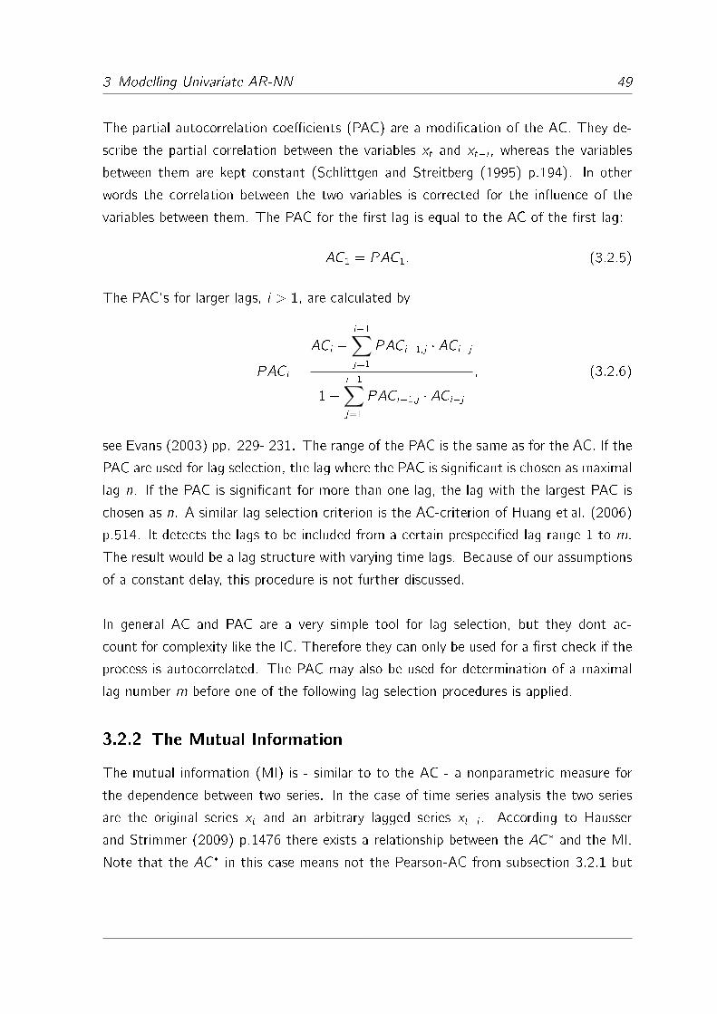
3 Modelling Univariate AR-NN 49
The partial autocorrelation coe�cients (PAC) are a modi�cation of the AC. They de-
scribe the partial correlation between the variables xt and xt�i , whereas the variables
between them are kept constant (Schlittgen and Streitberg (1995) p.194). In other
words the correlation between the two variables is corrected for the in�uence of the
variables between them. The PAC for the �rst lag is equal to the AC of the �rst lag:
AC1 = PAC1: (3.2.5)
The PAC's for larger lags, i > 1, are calculated by
PACi =
ACi �i�1∑j=1
PACi�1;j � ACi�j
1�i�1∑j=1
PACi�1;j � ACi�j
; (3.2.6)
see Evans (2003) pp. 229- 231. The range of the PAC is the same as for the AC. If the
PAC are used for lag selection, the lag where the PAC is signi�cant is chosen as maximal
lag n. If the PAC is signi�cant for more than one lag, the lag with the largest PAC is
chosen as n. A similar lag selection criterion is the AC-criterion of Huang et al. (2006)
p.514. It detects the lags to be included from a certain prespeci�ed lag range 1 to m.
The result would be a lag structure with varying time lags. Because of our assumptions
of a constant delay, this procedure is not further discussed.
In general AC and PAC are a very simple tool for lag selection, but they dont ac-
count for complexity like the IC. Therefore they can only be used for a �rst check if the
process is autocorrelated. The PAC may also be used for determination of a maximal
lag number m before one of the following lag selection procedures is applied.
3.2.2 The Mutual Information
The mutual information (MI) is - similar to to the AC - a nonparametric measure for
the dependence between two series. In the case of time series analysis the two series
are the original series xt and an arbitrary lagged series xt�i . According to Hausser
and Strimmer (2009) p.1476 there exists a relationship between the AC� and the MI.
Note that the AC� in this case means not the Pearson-AC from subsection 3.2.1 but

3 Modelling Univariate AR-NN 50
rater a general version of the AC which also accounts especially for nonlinearity (The
Pearson-AC is considered to be only a estimator of the true AC� in this case).
MIi = MI(xt ; xt�i) = �1
2log(1� AC�2
i ) (3.2.7)
The range of values of the MI is R+. It is symmetric (MI(xt ; xt�i)=MI(xt�i ; xt)) and
zero if the variable xt and its lag xt�i are independent (see Hausser and Strimmer (2009)
p.1476). Granger and Lin (1994) p. 375 use the relationship between the AC� and the
MI to formulate the MI coe�cient (MIC),
MICi = MIC(xt ; xt�i) = jAC�j =√1� e�2�MIi : (3.2.8)
The MIC of Granger and Lin (1994) is consequently an alternative estimator of the
absolute value of the autocorrelation coe�cient. Granger and Lin (1994) p.379- 383
show by simulation that their MIC does a better job in identifying the true lag order
than the Pearson-AC. The range of the MIC is between 0 and 1, because the MIC
approximates an absolute value.
The MI is de�ned as the joint Shannon-entropy H(xt ; xt�i) between the two variables,
subtracted the Shannon-entropy of each single variable (H(xt), H(xt�i)):
MIi = H(xt) +H(xt�i)�H(xt ; xt�i) (3.2.9)
To explain the Shannon entropy we �rst need the probability density function of the
variable xt . We will discuss those methods only for H(xt), but they can as well be
applied to calculate the Shannon entropy of xt�i and the Shannon entropy of the joint
data xt and xt�i . Granger and Lin (1994) p.375 propose to use kernel density esti-
mation to determine the probability density function, but in the case of discrete series
with a relatively small number of observations the ordinary histogram is su�cient. The
histogram is a discrete representation of the distribution. To determine the histogram,
the value range of the series is split into d bins. Let vi 8 i = 1; : : : ; d denote the number
of values of the original series xt belonging to the ith bin (for the well known frequency
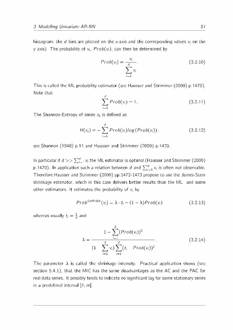
3 Modelling Univariate AR-NN 51
histogram, the d bins are plotted on the x-axis and the corresponding values vi on the
y-axis). The probability of vi , P rob(vi), can then be determined by
P rob(vi) =vid∑i=1
vi
: (3.2.10)
This is called the ML probability estimator (see Hausser and Strimmer (2009) p.1470).
Note thatd∑i=1
P rob(vi) = 1: (3.2.11)
The Shannon-Entropy of series xt is de�ned as
H(xt) = �d∑i=1
P rob(vi)log (P rob(vi)) : (3.2.12)
see Shannon (1948) p.11 and Hausser and Strimmer (2009) p.1470.
In particular if d >>∑d
i=1 vi the ML estimator is optimal (Hausser and Strimmer (2009)
p.1470). In application such a relation between d and∑d
i=1 vi is often not observable.
Therefore Hausser and Strimmer (2009) pp.1472-1473 propose to use the James-Stein
shrinkage estimator, which in this case delivers better results than the ML- and some
other estimators. It estimates the probability of vi by
P robSHRINK(vi) = � � ti + (1� �)P rob(vi) (3.2.13)
whereas usually ti =1dand
� =
1�d∑i=1
(P rob(vi))2
(1�d∑i=1
vi)
d∑i=1
(ti � P rob(vi))2
: (3.2.14)
The parameter � is called the shrinkage intensity. Practical application shows (see
section 5.4.1), that the MIC has the same disadvantages as the AC and the PAC for
real data series. It possibly tends to indicate no signi�cant lag for some stationary series
in a prede�ned interval [1;m].
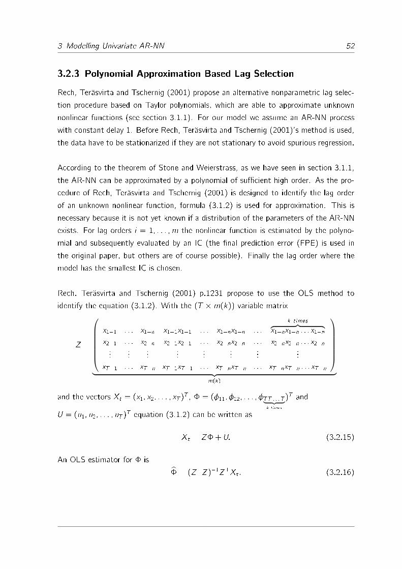
3 Modelling Univariate AR-NN 52
3.2.3 Polynomial Approximation Based Lag Selection
Rech, Teräsvirta and Tschernig (2001) propose an alternative nonparametric lag selec-
tion procedure based on Taylor polynomials, which are able to approximate unknown
nonlinear functions (see section 3.1.1). For our model we assume an AR-NN process
with constant delay 1. Before Rech, Teräsvirta and Tschernig (2001)'s method is used,
the data have to be stationarized if they are not stationary to avoid spurious regression.
According to the theorem of Stone and Weierstrass, as we have seen in section 3.1.1,
the AR-NN can be approximated by a polynomial of su�cient high order. As the pro-
cedure of Rech, Teräsvirta and Tschernig (2001) is designed to identify the lag order
of an unknown nonlinear function, formula (3.1.2) is used for approximation. This is
necessary because it is not yet known if a distribution of the parameters of the AR-NN
exists. For lag orders i = 1; : : : ; m the nonlinear function is estimated by the polyno-
mial and subsequently evaluated by an IC (the �nal prediction error (FPE) is used in
the original paper, but others are of course possible). Finally the lag order where the
model has the smallest IC is chosen.
Rech, Teräsvirta and Tschernig (2001) p.1231 propose to use the OLS method to
identify the equation (3.1.2). With the (T �m(k)) variable matrix
Z =
x1�1 : : : x1�n x1�1x1�1 : : : x1�nx1�n : : :
k times︷ ︸︸ ︷x1�nx1�n : : : x1�n
x2�1 : : : x2�n x2�1x2�1 : : : x2�nx2�n : : : x2�nx2�n : : : x2�n...
......
......
......
...
xT�1 : : : xT�n xT�1xT�1 : : : xT�nxT�n : : : xT�nxT�n : : : xT�n
︸ ︷︷ ︸
m(k)
and the vectors Xt = (x1; x2; : : : ; xT )T , � = (�11; �12; : : : ; �TT : : : T| {z }
k times
)T and
U = (u1; u2; : : : ; uT )T equation (3.1.2) can be written as
Xt = Z�+ U: (3.2.15)
An OLS estimator for � is
� = (Z>Z)�1Z>Xt : (3.2.16)

3 Modelling Univariate AR-NN 53
Therewith a polynomial approximation of the unknown AR-NN function is given by
xt =
n∑j1=1
�j1xt�j +n∑
j1=1
n∑j2=j1
�j1;j2xt�j1xt�j2
+
n∑j1=1
n∑j2=j1
n∑j3=j2
�j1;j2;j3xt�j1xt�j2xt�j3 +
n∑j1=1
: : :
n∑jk=jk�1
�j1;j2;:::;jkxt�j1 : : : xt�jk + ut
whereas �j1,: : :,�j1;j2;:::;jk are the elements of �. Now it is easy to calculate the AIC or
BIC for this equation to identify the optimal lag order. Like in linear equations, it is
observable in practical application, that the AIC tends to include more lags than the
BIC (see section 5.4.1). For application we suggest to use a polynomial of order three,
which should be su�cient as it was already proposed by Lee, White and Granger (1993).
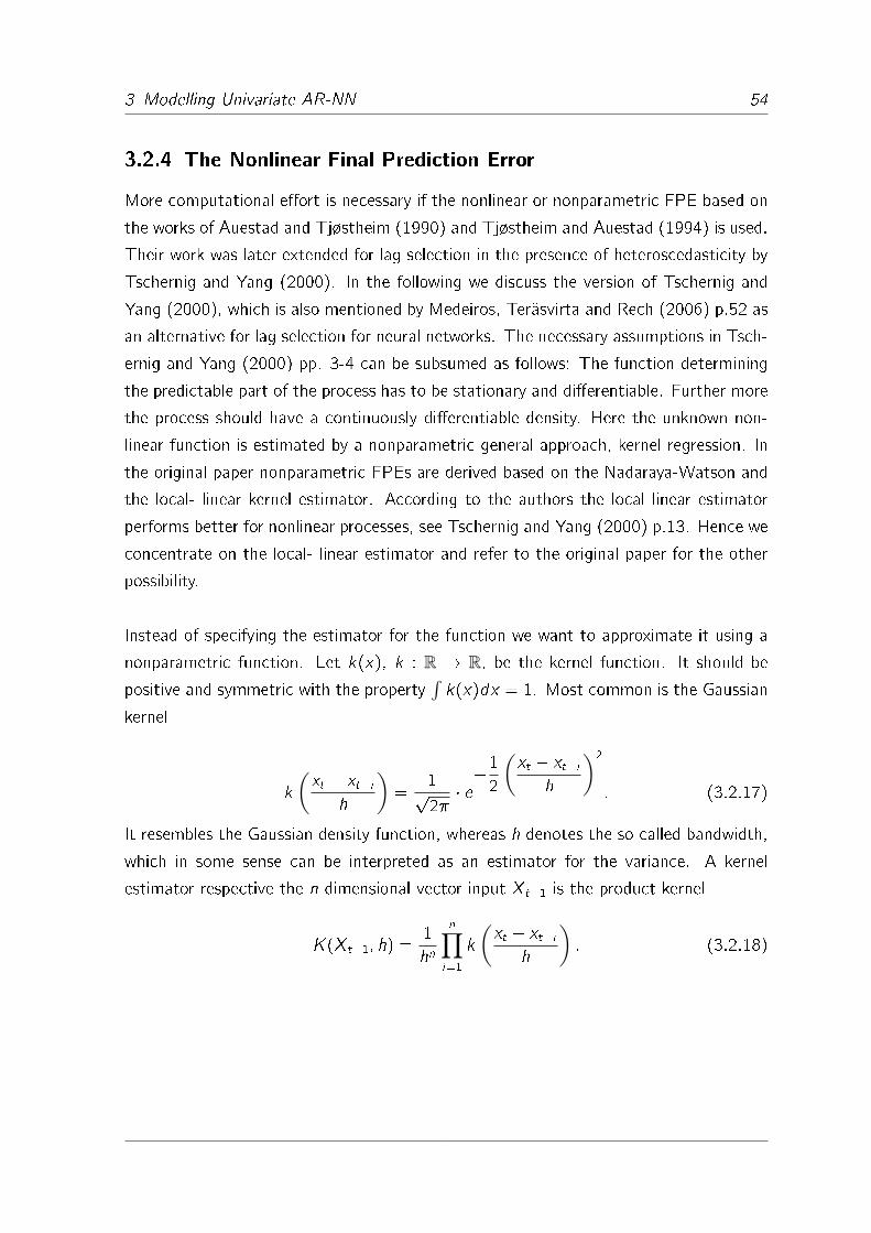
3 Modelling Univariate AR-NN 54
3.2.4 The Nonlinear Final Prediction Error
More computational e�ort is necessary if the nonlinear or nonparametric FPE based on
the works of Auestad and Tjøstheim (1990) and Tjøstheim and Auestad (1994) is used.
Their work was later extended for lag selection in the presence of heteroscedasticity by
Tschernig and Yang (2000). In the following we discuss the version of Tschernig and
Yang (2000), which is also mentioned by Medeiros, Teräsvirta and Rech (2006) p.52 as
an alternative for lag selection for neural networks. The necessary assumptions in Tsch-
ernig and Yang (2000) pp. 3-4 can be subsumed as follows: The function determining
the predictable part of the process has to be stationary and di�erentiable. Further more
the process should have a continuously di�erentiable density. Here the unknown non-
linear function is estimated by a nonparametric general approach, kernel regression. In
the original paper nonparametric FPEs are derived based on the Nadaraya-Watson and
the local- linear kernel estimator. According to the authors the local linear estimator
performs better for nonlinear processes, see Tschernig and Yang (2000) p.13. Hence we
concentrate on the local- linear estimator and refer to the original paper for the other
possibility.
Instead of specifying the estimator for the function we want to approximate it using a
nonparametric function. Let k(x), k : R ! R, be the kernel function. It should be
positive and symmetric with the property∫k(x)dx = 1. Most common is the Gaussian
kernel
k
(xt � xt�i
h
)=
1p2�
� e�1
2
(xt � xt�i
h
)2
: (3.2.17)
It resembles the Gaussian density function, whereas h denotes the so called bandwidth,
which in some sense can be interpreted as an estimator for the variance. A kernel
estimator respective the n dimensional vector input Xt�1 is the product kernel
K(Xt�1; h) =1
hn
n∏i=1
k
(xt � xt�i
h
): (3.2.18)
3 Modelling Univariate AR-NN 55
For the de�nition of the local linear estimator for F (Xt�1) we need the following vectors
and matrices:
Z =
(1 1 : : : 1
Xn�1 �Xt�1 Xn�2 �Xt�1 : : : Xn�T �Xt�1
)>
(3.2.19)
W = diag
{K(Xj�1 �Xt�1; h)
T � n + 1
}T
j=n
(3.2.20)
E = (1; 0; : : : ; 0)> (3.2.21)
Y = (xn; : : : ; xT )> (3.2.22)
The dimensions are ((n+1)� 1) for E, ((T � n+1)� (n+1)) for Z, ((T � n+1)�(T � n + 1)) for W and ((T � n + 1) � 1) for Y . The matrix in (3.2.20) denotes a
diagonal matrix with a diagonal of length (T � n + 1) with
(K(Xj�1 �Xt�1; h)
T � n + 1
)at
the jth element for j = n : : : T . The local linear estimator for the unknown function
F (Xt�1) is
F (Xt�1; h) = E> {Z>WZ}�1
Z>WY: (3.2.23)
The nonparametric version of the FPE, called Asymptotic FPE (AFPE) is calculated
by
AFPE(Xt�1; hopt ; hB) = A(hopt) + 2K(0)n1
(T � n + 1)hnopt� B(hB); (3.2.24)
whereas
A(hopt) =1
T � n + 1
T∑i=n
(xt � F (Xt�1; hopt)
)w(Xm�t) (3.2.25)
and
B(hB) =1
T � n + 1
T∑i=n
(xt � F (Xt�1; hB)
) w(Xm�t)�(Xt�1; hB)
: (3.2.26)
3 Modelling Univariate AR-NN 56
The function w(Xm�t) depends of the prespeci�ed maximal lag m and �(Xt�1; hB) is
a kernel density estimator calculated by
�(Xt�1; hB) =1
T � n + 2
T+1∑i=n
K(Xi�1 �Xt�1; hB): (3.2.27)
The �rst term of equation (3.2.24) can be considered as the performance term whereas
the second term is the penalty term (Härdle, Kleinow and Tschernig (2001) p.4). For
calculation of the plug-in bandwidth hopt used in (3.2.25) we refer to Tschernig (2005)
p.10. The bandwidth hB is determined by the rule of Silverman (1986) pp.86-87, see
also Tschernig (2005) pp.9-10:
hB = 2�
(4
n + 4
) 1
n+6
T� 1
n+6 (3.2.28)
� is the geometric mean of the standard deviations of the regressors,
� =
(n∏i=1
√�2xt�i
) 1
n
; (3.2.29)
whereas �2xt�i
is the variance of the lag (or regressor) xi . The lag selection procedure
is executed as follows: First the maximal lag order m has to be prespeci�ed and subse-
quently the AFPEs for all lag orders n = 1; : : : ; m have to be calculated. The optimal
lag order has the smallest AFPE.
Tschernig and Yang (2000) p.9 mention, that the AFPE tends to include too many
lags (over�tting). Thus they propose an extension of the AFPE, the corrected AFPE
(CAFPE), which accounts for that problem:
CAFPE = AFPE(1 + n(T � n)�
4
m+4
)(3.2.30)
Like the AFPE the CAFPE has to be minimized. Medeiros, Teräsvirta and Rech (2006)
p.52 state that computation of the AFPE or CAFPE may become very e�ortly, in
particular if T and m become large. Thus this procedure may be appropriate especially
for small maximal lag numbersm. Already Auestad and Tjøstheim (1990) p.686 observe
by simulation, that their version of the nonlinear FPE works only accurate for 3-4 lags
in a time series with T = 500 observations.

3 Modelling Univariate AR-NN 57
3.3 Parameter Estimation
The most important step to concretize the AR-NN is the estimation of the weights.
This equals the estimation of the parameters in linear time series analysis and is called
learning or training in neural network theory. Many procedures exist to estimate the
parameters of neural networks. Thus it has to be distinguished between supervised
learning methods und unsupervised methods (Haykin (2009) pp.64-67). Supervised
methods means that the estimation output is compared to a desired output and esti-
mation takes the error signal into account. The error signal is de�ned as the di�erence
between estimation and desired output. Unsupervised methods use no criteria to control
the learning process, so they seem not applicable to statistics and especially time series
analysis. Hence in the following we concentrate on supervised learning procedures only.
In general it can be said that there are two di�erent classes of supervised learning pro-
cedures concerning the estimation of the parameters (see Widmann (2000) pp.28-29,
Haykin (2009) pp.157-159). Batch learning is an iterative procedure where the weights
are adjusted in each iteration after the presentation of all T inputs, while during on-line
learning - sometimes referred to as stochastic learning - the weights are adjusted on
element-by-element basis. This means that for each set of input and output neurons
from 1 to T the weights are newly adjusted. The AR-NN process is estimated for the
inputs and outputs at a certain time t only, for time t + 1 the weights are adjusted
again. The main advantages of on-line over batch learning methods are the lower com-
putational complexity and the better adaptability to integrate new values if data arrive
sequentially.
Some studies have shown that under certain conditions batch and on-line learning pro-
cedures deliver similar results particularly if the input data set is large (Oppner (1998)
p.363). In general it can be said that on-line learning is faster and less complex
than batch learning, but concerning the precision of the results it performs poor (Bot-
tou (2003) p.172). Hence on-line learning might be more useful in electrical engineering
where complexity matters much more than in statistics and particularly time series anal-
ysis, where the focus is on comprising long term patterns the most precise way out of
a closed historical data set.

3 Modelling Univariate AR-NN 58
Hence in the following we proceed with batch learning procedures only, notwithstanding
that in the last years several proceedings have been made concerning the performance
of on-line learning procedures in pattern recognition (for example Schraudolph (2002)
etc.). We do so because in statistics generally the data sets are completely delivered
and contains all the necessary information to analyze the long term interdependencies.
On-line learning procedures would be useful if input data were provided continuously,
even during the learning process, and therefore the adjustment of the weights has to be
an evolving process. A main problem is that on-line algorithms do not really converge,
because they are adjusted after each new input of a variable set. The most advanta-
geous property of batch learning is its accurate estimation of the gradient vector for a
�nite input data set, which guarantees the convergence of the algorithms presented in
the following. Hence according to White (1989c) p.1005 batch learning is more e�cient
than on-line learning from a statistical point of view.
The supervised batch learning algorithms in the subsequent sections are iterative nu-
meric procedures, which possibly lead only to local minima. Direct methods similar to
the OLS method can not be implemented for AR-NN as they are not able to account
for the nonlinear part of the function. However Medeiros, Teräsvirta and Rech (2006)
pp.53-55 propose a hybrid method where the linear part of an AR-NN is estimated us-
ing the maximum-likelihood method for linear models. A numeric method estimates the
remaining nonlinear part. For example Widmann (2000) pp.65-66 discusses some pro-
cedures (simulated annealing and generic algorithms) which claim to be able to identify
a global minimum for nonlinear functions. But such procedures do not only require too
much e�ort to be of any use for our purposes (Anders (1997) p.36) but it is also ques-
tionable if they can keep their promise and lead to a global minimum at least in �nite
time (White (1992) pp.111-112, Widmann (2000) p.34). Thus we only concentrate on
the local search methods, which are well established in the neural network literature.
3.3.1 The Performance Function
The performance function we use is rooted in White (1989b) pp.430- 433 (see also
Trapletti, Leisch and Hornik (2000) pp.2437-2442 and Widmann (2000) pp.32- 34).

3 Modelling Univariate AR-NN 59
Like in the well known least square procedures the goodness of �t of an AR-NN model
can be determined by
Q(�) =1
2
T∑t=1
(xt � G(�; Xt�1))2: (3.3.1)
If this performance function is used, the parameter estimation procedures in the follow-
ing are referred to as nonlinear least squares (NLS) method in literature and are not
restricted to neural networks only. Of course it is possible to use other performance
functions like the likelihood function (see Anders (1997) pp.23-25), but they are less
common. As the AR-NN function should also be valid for future values of the time
series, the expectation of fuction (3.3.1) has to be minimized. As an AR in general is
a stochastic process, there is some uncertainty as we know from de�nition 2.1. We
assume that the uncertainty is only determined by the stochastic part "t . This uncer-
tainty should be minimized. Due to our assumptions on "t (i.i.d. Gaussian distributed
with zero mean and constant variance) this is the case if its variance is minimized. The
relationship between the performance function and the variance of "t as well as the fact
that minimization of the one equals the minimization of the other is formally shown in
the following.
The uncertainty also causes the stochastic property of the expectation, which is the rea-
son that one can not calculate � directly but has to estimate it. An optimal nonlinear
least squares estimator for �, �, can be found by solution of the problem
� = argmin�2�
E(Q(�)); (3.3.2)
� denotes the network weight space.
By transformation of Q(�) one can show that an optimal � � � is minimizing the ex-

3 Modelling Univariate AR-NN 60
pected error between an unknown function F (Xt�1) and its approximation G(�; Xt�1)
(White (1988) p.432):
E(Q(�)) =1
2E[
T∑t=1
(xt � G(�; Xt�1))2]
=1
2E[
T∑t=1
((xt � F (Xt�1) + F (Xt�1))� G(�; Xt�1))2)]
=1
2E[
T∑t=1
(xt � F (Xt�1)2)] +
1
22E[
T∑t=1
(xt � F (Xt�1))(F (Xt�1)� G(�; Xt�1)))]
+1
2E[
T∑t=1
((F (Xt�1)� G(�; Xt�1)2)] (3.3.3)
=1
2E[
T∑t=1
((xt � F (Xt�1)2)] +
1
2E[
T∑t=1
((F (Xt�1)� G(�; Xt�1)2)] (3.3.4)
=1
2E[
T∑t=1
"2t ] +1
2E[
T∑t=1
((F (Xt�1)� G(�; Xt�1)2)]: (3.3.5)
(3.3.4) follows from (3.3.3) because
E[
T∑t=1
((xt � F (Yt))(F (Xt�1)� G(�; Xt�1))]
= E[
T∑t=1
((xt � F (Xt�1))"t)]
= E[
T∑t=1
(E(xt � F (Xt�1))"t jXt�1)]
= E[
T∑t=1
((xt � F (Xt�1))E("t jXt�1))]
= 0
Note that E("t jXt�1) = 0 8 t. The �rst term of (3.3.5) states that � minimizes the
errors of the stochastic part. The second term states that a for Q(�) a minimum is
3 Modelling Univariate AR-NN 61
reached if G(�; Xt�1) = F (Xt�1). In this case (3.3.5) reduces to (with respect to the
i.i.d. assumption)
Q(�) =1
2
T∑t=1
"2t : (3.3.6)
This causes on the other hand the statement (see therefore equation (3.3.1))
T∑t=1
"t =
T∑t=1
(xt � G(�; Xt�1)) (3.3.7)
and
"t = "t(�) = (xt � G(�; Xt�1)): (3.3.8)
In equation (3.3.8) the residual at time t is described by a function of �. This function
as well as the performance function are important for the following sections.
3.3.2 Important Matrix Terms
In the following sections we will extensively use the constructs gradient vector, Jacobian
matrix and Hessian matrix. Hence they should be introduced and explained here. The
aim is to impart understanding of the dimensionality in the following.
The simplest construct is the gradient vector, indicated by r(�). The gradient vec-
tor is a column vector of the partial derivatives of a function respective its variables.
Consider for example the gradient vector of the performance function:
rQ(�) =
@Q(�)
@�1...
@Q(�)
@�r
(3.3.9)
Its dimension is (r � 1). If a function additionally depends on time t, for example the
residual at time t in equation (3.3.8), the Jacobian matrix corresponds in some sense
to the gradient vector. It is the matrix of the partial derivatives respective the variables
3 Modelling Univariate AR-NN 62
(in the rows) and the time (in the columns). We denote it by J(�). For equation (3.3.8)the Jacobian matrix has dimension (T � r) and is calculated by:
J("t(�)) =
@"1@�1
@"1@�2
: : :@"1@�r
@"2@�1
@"2@�2
: : :@"2@�r
.... . .
...
@"T@�1
@"T@�2
: : :@"T@�r
: (3.3.10)
There is a relationship between the gradient vector of the performance function and
the Jacobian matrix of (3.3.8) which can be constructed using the residual vector
E = ("1; "2; : : : ; "T ). The (r � 1)-dimensional gradient vector rQ(�) is the product
of the transposed Jacobian matrix J("t(�)) of dimension (r � T ) and the (T � 1)-
dimensional vector E.
rQ(�) = J("t(�))>E =
"1@"1@�1
+ "2@"2@�1
+ : : : + "T@"T@�1
"1@"1@�2
+ "2@"2@�2
+ : : : + "T@"T@�2
......
......
"1@"1@�r
+ "2@"2@�r
+ : : : + "T@"T@�r
(3.3.11)
Note that this relationship is in particular 8 i = 1; : : : ; r based on (3.3.6) because
@Q(�)
�i= r1
2
(T∑t=1
"2t
)= 2 � 1
2
(T∑t=1
"t
) @
(T∑t=1
"t
)@�i
: (3.3.12)

3 Modelling Univariate AR-NN 63
The third important matrix term is the Hessian matrix. It is the matrix of second order
derivatives of a function respective its input variables and is denoted by r2(�). For theperformance function Q(�) it has the following (r � r) representation:
r2Q(�) =
@2Q(�)
@�1@�1
@2Q(�)
@�1@�2: : :
@2Q(�)
@�1@�r
@2Q(�)
@�2@�1
@2Q(�)
@�2@�2: : :
@2Q(�)
@�2@�r
......
. . ....
@2Q(�)
@�r@�1
@2Q(�)
@�r@�2: : :
@2Q(�)
@�r@�r
(3.3.13)
3.3.3 Basic Features of the Algorithms
All numeric parameter estimation algorithms for neural networks work the same way:
Starting with a random initial parameter vector �0 it is searched iteratively for the
optimal parameter vector. The optimal parameter vector is reached if the performance
function is minimized. To show how the search direction is determined the performance
function is depicted in �gure 3.3 as a function of �i, whereas i indicates the number of
the iteration, starting with i=0. The function has various extrema, minima as well as
maxima, which satisfy rQ(�) = 0 (Bishop (1995) pp.254-255), because the gradient
rQ(�) is the slope of the function.
However sometimes only a local minimum might be reached by the algorithm. In addi-
tion the choice of the initial weight vector �0 in�uences the outcome of the algorithm
respective local and global minima. But as already discussed above, there are no alter-
native algorithms which guarant to �nd a global minimum.
In general the algorithm is carried out according to the �ow chart in �gure 3.4. The
weights are updated after each iteration and the performance function is calculated. If
a stopping criterion is reached, the algorithm is quitted. The stopping criterion can be
a restriction concerning the performance function, for example the distance between
performance function in two iterations, which should be below a certain value (see An-
ders (1997) p.36). For our attempt such a stopping criterion eventually circumvents

3 Modelling Univariate AR-NN 64
the detection of a better minimum, because the algorithm is stopped immediately after
the criterion is achieved. Thus we recommend saving the result of the performance
function and the parameter vector after each iteration. Then the maximal number of
iterations imax can be used as a stopping criterion and the optimal parameter vector is
calculated by the following steps:
� Start the algorithm with the initial weight vector �0
� After each iteration save Q(�i) and �i
� Quit the algorithm after imax iterations
� Among the saved values search
Q(�i*) = argmini2[0;imax ]
Q(�i)
� �i* is the optimal parameter vector
i* denotes the iteration where the optimal parameter vector is reached. Such a pro-
cedure can be interpreted as search for a global minimum within a �nite horizon of
iterations. One critical point is the need for storage for each iteration, but to our at-
tempt this is outweighed by the fact that this procedure is able to identify a very good
local minimum. Often the performance function converges to a certain constant within
a �nite number of iterations. Therefore a good local minimum within a �nite number
of iterations, imax , often is in fact a global minimum. Thus we prefer this method in
the following. It is implemented in context with the Levenberg-Marquardt algorithm in
R in appendix B.4.
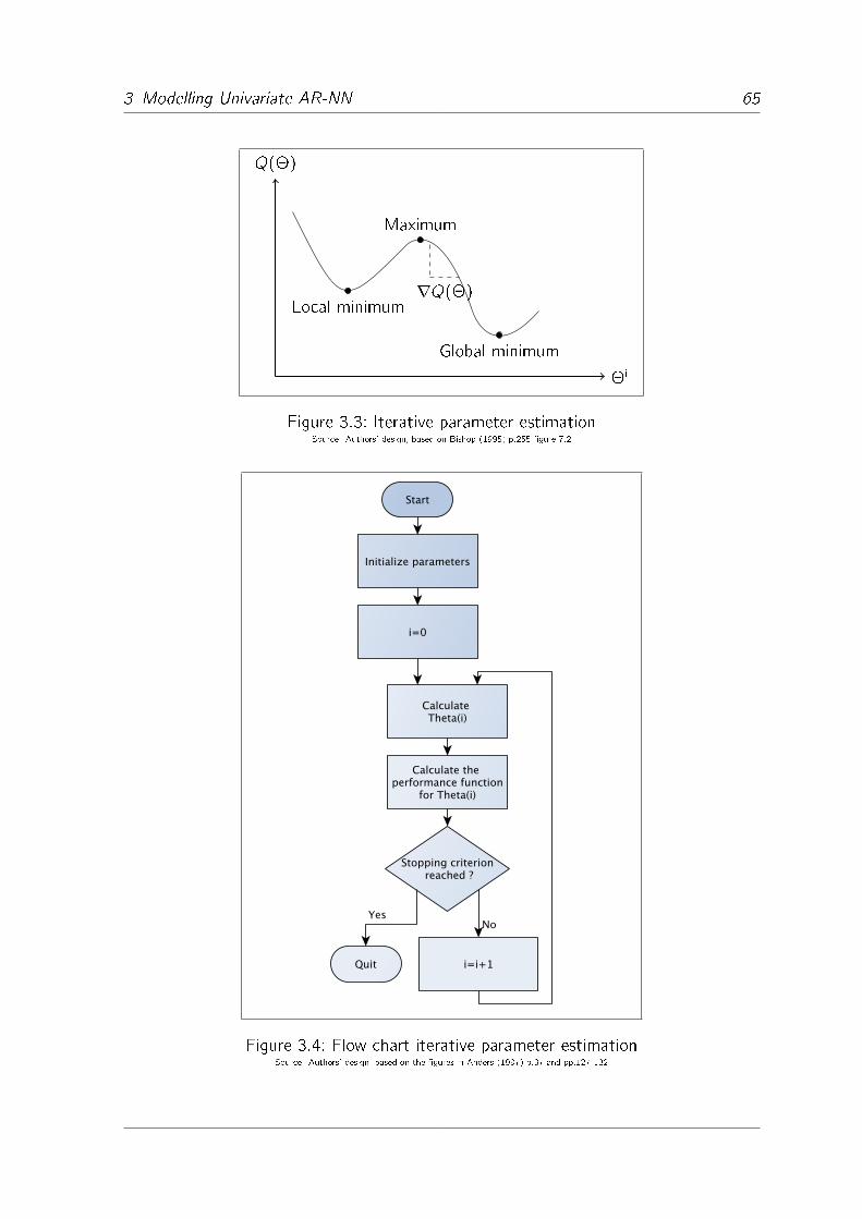
3 Modelling Univariate AR-NN 65
�i
Q(�)
Local minimum
Maximum
Global minimum
rQ(�)
Figure 3.3: Iterative parameter estimationSource: Authors' design, based on Bishop (1995) p.255 �gure 7.2
Figure 3.4: Flow chart iterative parameter estimationSource: Authors' design, based on the �gures in Anders (1997) p.37 and pp.127-132
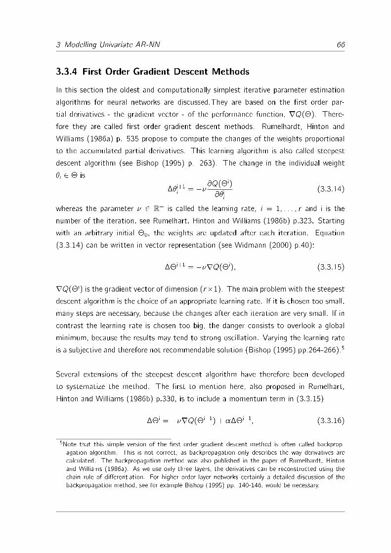
3 Modelling Univariate AR-NN 66
3.3.4 First Order Gradient Descent Methods
In this section the oldest and computationally simplest iterative parameter estimation
algorithms for neural networks are discussed.They are based on the �rst order par-
tial derivatives - the gradient vector - of the performance function, rQ(�). There-
fore they are called �rst order gradient descent methods. Rumelhardt, Hinton and
Williams (1986a) p. 535 propose to compute the changes of the weights proportional
to the accumulated partial derivatives. This learning algorithm is also called steepest
descent algorithm (see Bishop (1995) p. 263). The change in the individual weight
�i 2 � is
��i+1i = �� @Q(�
i)
@�ii(3.3.14)
whereas the parameter � 2 R+ is called the learning rate, i = 1; : : : ; r and i is the
number of the iteration, see Rumelhart, Hinton and Williams (1986b) p.323. Starting
with an arbitrary initial �0, the weights are updated after each iteration. Equation
(3.3.14) can be written in vector representation (see Widmann (2000) p.40):
��i+1 = ��rQ(�i); (3.3.15)
rQ(�i) is the gradient vector of dimension (r�1). The main problem with the steepest
descent algorithm is the choice of an appropriate learning rate. If it is chosen too small,
many steps are necessary, because the changes after each iteration are very small. If in
contrast the learning rate is chosen too big, the danger consists to overlook a global
minimum, because the results may tend to strong oscillation. Varying the learning rate
is a subjective and therefore not recommendable solution (Bishop (1995) pp.264-266).5
Several extensions of the steepest descent algorithm have therefore been developed
to systematize the method. The �rst to mention here, also proposed in Rumelhart,
Hinton and Williams (1986b) p.330, is to include a momentum term in (3.3.15)
��i = ��rQ(�i�1) + ���i�1; (3.3.16)
5Note that this simple version of the �rst order gradient descent method is often called backprop-
agation algorithm. This is not correct, as backpropagation only describes the way derivatives are
calculated. The backpropagation method was also published in the paper of Rumelhardt, Hinton
and Williams (1986a). As we use only three layers, the derivatives can be reconstructed using the
chain rule of di�erentiation. For higher order layer networks certainly a detailed discussion of the
backpropagation method, see for example Bishop (1995) pp. 140-146, would be necessary.
3 Modelling Univariate AR-NN 67
where � 2 [0; 1] is the momentum parameter and the last term is called the momen-
tum term. The reason why this term is added is that it can �lter out high frequency
variations in the error-surface in the weight space. In other words the momentum term
"smoothens" the oscillations. The e�ect is faster convergence of the algorithm, because
one can use larger � without the danger of missing any global minimum (Rumelhart,
Hinton and Williams (1986b) p.330). According to Bishop (1995) p.268 this extension
does not really solve the problems of the simple gradient descent algorithm of equation
(3.3.15), because it depends on a second parameter, �, which has to be chosen arbi-
trary like �.
Another alternative is the so called bold-driver method of Vogl et al. (1988), where
the learning rate is updated according to some rules after each iteration, for the follow-
ing see Vogl et al. (1988) p.259 and Bishop (1995) p.269. Consider equation (3.3.15):
If the value of the present error function Q(�i) is smaller than that of the previous
error function Q(�i�1), the learning rate can be slightly increased in the next itera-
tion. This is done by multiplication by a parameter �1, which is slightly above 1, for
example �1 = 1:1. If the value of the present error function is bigger than that of the
previous error function, the learning rate has to be decreased and the iteration has to
be repeated, because it can be possible that a global minimum has been overlooked.
Therefore � is set 0 and � is multiplied by a parameter �2, which has to be signi�cantly
less than 1, for example �2 = 0:5.
A modi�cation of the bold-driver method is the delta-bar-delta-rule proposed by Ja-
cobs (1988) pp.299-301. A local gradient �delta� is de�ned for iteration i and weight i
as
�ii =@Q(�i)
@�ii: (3.3.17)
The extension of that local gradient, �delta-bar�, is
��ii = (1� �1)�ii + �1
��i�1i : (3.3.18)
The learning rate update is computed using (3.3.17) and (3.3.18) by
�� ii =
�2 if ��i�1i �ii > 0
��3�ii if ��i�1
i �ii < 0: (3.3.19)
3 Modelling Univariate AR-NN 68
Note that this method implies, that each element of the weight vector is updated in-
dividually like in the bold-driver algorithm. The system behind this approach is on the
one hand to increase the learning rates in a linear way and thus to avoid a too rapid
increase. On the other hand the learning rate is decreased exponentially to ensure that
no global minimum is missed. One disadvantage of this method is, that three parame-
ters (�1; �2; �3) have to be determined, if a momentum term is added four parameters.
The other disadvantage is, that the weight parameters are treated like they were inde-
pendent, which actually is often not the case (Bishop (1995) p.271).
Another class of �rst order gradient descent methods are the so called line search meth-
ods (Bishop (1995) p.272-274). They are at least an extension of the gradient-reuse
algorithm of Hush and Salas (1988). The di�erence to the ordinary steepest descent
algorithm is, that the search direction is not determined only by the negative local gra-
dient but also by the weight space. Gradients are �reused� to update the learning rate.
Formally this can be written by using
��i+1 = �� irQ(�i)
�i+1 = �i � � irQ(�i); (3.3.20)
whereas the parameter � i is the parameter which minimizes
Q(� i) = Q(�i � � irQ(�i)): (3.3.21)
According to Widmann (2000) p.40 one avoids therewith to go arbitrary far in the di-
rection of the gradient. The learning rate � i leads to the deepest point in this direction.
There are two practical approaches to �nd the minimum of (3.3.21): The �rst is a
quadratic interpolation, which in a �rst stage computes three values of �, a < b < c
such that Q(a)>Q(b) and Q(c)>Q(b). If the error function is continuous, it is guar-
anteed that a minimum is between a and c . The second stage is the location of the
minimum by adjusting a quadratic polynomial to the error function at the points a,b and
c and searching for a minimum of that function (Bishop (1995) p.273). The alternative
approach is the computation of the derivatives of (3.3.21). This requires much more
computational e�ort and would in fact result in a second order gradient descent method
(Widmann (2000) p.41).
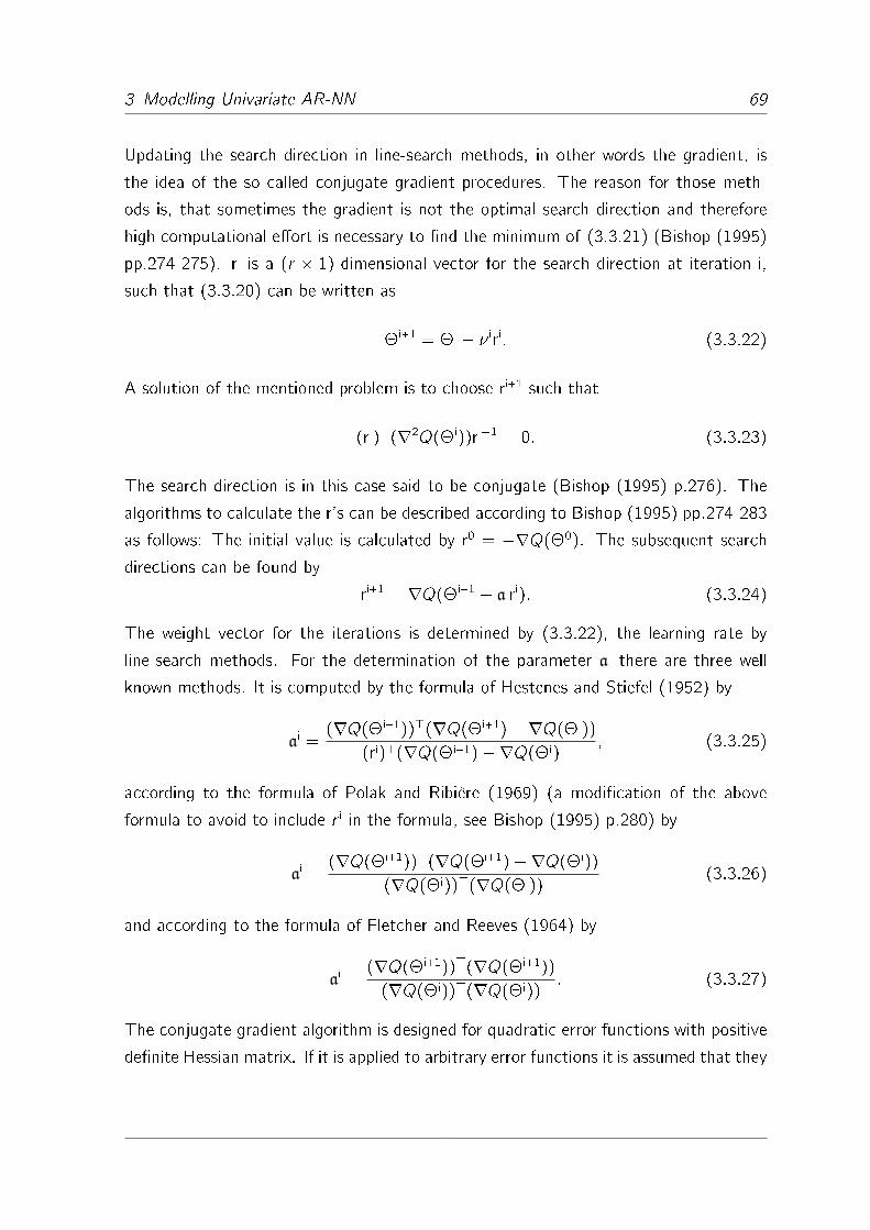
3 Modelling Univariate AR-NN 69
Updating the search direction in line-search methods, in other words the gradient, is
the idea of the so called conjugate gradient procedures. The reason for those meth-
ods is, that sometimes the gradient is not the optimal search direction and therefore
high computational e�ort is necessary to �nd the minimum of (3.3.21) (Bishop (1995)
pp.274-275). ri is a (r � 1)-dimensional vector for the search direction at iteration i,
such that (3.3.20) can be written as
�i+1 = �i � � iri: (3.3.22)
A solution of the mentioned problem is to choose ri+1 such that
(ri)>(r2Q(�i))ri�1 = 0: (3.3.23)
The search direction is in this case said to be conjugate (Bishop (1995) p.276). The
algorithms to calculate the r's can be described according to Bishop (1995) pp.274-283
as follows: The initial value is calculated by r0 = �rQ(�0). The subsequent search
directions can be found by
ri+1 = rQ(�i+1 + airi): (3.3.24)
The weight vector for the iterations is determined by (3.3.22), the learning rate by
line-search methods. For the determination of the parameter ai there are three well
known methods. It is computed by the formula of Hestenes and Stiefel (1952) by
ai =(rQ(�i+1))>(rQ(�i+1)�rQ(�i))
(ri)>(rQ(�i+1)�rQ(�i); (3.3.25)
according to the formula of Polak and Ribière (1969) (a modi�cation of the above
formula to avoid to include r i in the formula, see Bishop (1995) p.280) by
ai =(rQ(�i+1))>(rQ(�i+1)�rQ(�i))
(rQ(�i))>(rQ(�i))(3.3.26)
and according to the formula of Fletcher and Reeves (1964) by
ai =(rQ(�i+1))>(rQ(�i+1))
(rQ(�i))>(rQ(�i)): (3.3.27)
The conjugate gradient algorithm is designed for quadratic error functions with positive
de�nite Hessian matrix. If it is applied to arbitrary error functions it is assumed that they

3 Modelling Univariate AR-NN 70
can be locally approximated by a quadratic polynomial, but they dont have necessarily
to be quadratic. The formula of Polak and Ribière (1969) is superior in the case of
nonlinear error functions (Haykin (2009) p.222). But continuing this discussion would
lead too far as we only use the quadratic error function (3.3.1). The conjugate-gradient
method is generally the most powerful �rst order gradient descent method (if we abstain
from quasi-Newton methods mentioned in the next chapter).
3.3.5 Second Order Gradient Descent Methods
The second order gradient descent methods are learning algorithms, which explicitly
make use of the Hessian matrix r2Q(�). Consider equation (3.3.14): The learning
rate � is replaced by the inverse Hessian matrix such that
�i+1 = �i � (r2Q(�i))�1r(�i): (3.3.28)
The second term in this equation is called Newton direction. Its main advantage is,
that the Newton direction or Newton step of a quadratic error function directly points
towards a minimum and hence avoids oscillation (Bishop (1995) p. 286).
However determining the Hessian matrix brings along some problems. Firstly, it is
very demanding from a computational point of view to calculate and invert the Hessian
matrix. To show this, let O denote the Landau symbol indicating the upper bound of
the computing complexity. Computing the Hessian matrix has complexity O(r 2) and
inverting it O(r 3) (Bishop (1995) p.287). Secondly, the Newton direction may point
to a maximum or saddle point, which is the case if the Hessian matrix is not positive
de�nite. As a consequence the error is not necessary reduced in each iteration. Thirdly,
the step size of the Newton step may be such large that it leads out of the range of
validity.
The second problem can be reduced by adding a positive de�nite symmetric matrix
to the Hessian matrix which includes the unit Matrix I and a su�cient large parameter
�. Then the combination
r2Q(�) + �I (3.3.29)
is certainly positive de�nite. This is a compromise between the negative gradient search
direction, which (approximatively) results if � is chosen large, and the Newton direction,

3 Modelling Univariate AR-NN 71
which results if � is very small. In this way also the third problem mentioned above is
solved. But the �rst problem remains, which is in general known as the greatest disad-
vantage of the Newton's method and is the origin of several approximation procedures
called quasi-Newton methods. Because they do not deal with second order gradients
directly but approximate them via �rst order gradients, they are in general classi�ed
as �rst order gradient methods (Bishop (1995) pp.287-290, Widmann (2000) pp.44-
45, Haykin (2009) pp.224-226). We will not discuss those methods here and refer to
the literature mentioned above as with the Levenberg-Marquardt algorithm in the next
chapter a powerful kind of a quasi-Newton method is shown.
Shortly we want to compare the quasi-Newton and conjugate gradient methods (see
Haykin (2009) p.226-227): The complexity of conjugate gradient is only O(r), thus thismethod is preferable to quasi-Newton methods with an overall computing complexity of
O(r 2) (Haykin (2009) p.227) if the weight vector becomes large. An additional argu-
ment to that point of view is, that storage is required for the approximated Hessian ma-
trices which of course becomes the larger the more elements are included in the weight
vector. In the close neighborhood of a local minimum however, quasi-Newton methods
converge faster as they approximate Newton's method accurate. Quasi-Newton, conju-
gate gradient and the Levenberg-Marquardt algorithm converge with superlinear speed,
whereas the other methods converge with linear speed (Bottou (2003) pp. 165-166).
3.3.6 The Levenberg-Marquardt Algorithm
In the following we continue with the Levenberg- Marquardt algorithm (founded in the
works of Levenberg (1944) and Marquardt (1963)) which combines the steepest de-
scent algorithm of Rumelhart, Hinton and Williams (1986b) and Newton's method.
Like other quasi-Newton methods it can not be counted to the second order gradient
methods, because the Hessian matrix is approximated by combinations of the Jacobian
matrix of "t(�), the matrix of �rst oder gradients, such that no second order gradients
rest to calculate. According to Haykin (2009) p.227 the advantages of this method
are therefore that it converges rapidly like Newton's method but it can not diverge be-
cause of the steepest descent algorithm in�uence. Via modi�cation of some parameters
the Levenberg-Marquardt algorithm can be made equal to either the steepest descent-
or Newton's algorithm. The algorithm is also recommended in several econometric
works as for example in Medeiros, Teräsvirta and Rech (2006) p.54 and is commonly

3 Modelling Univariate AR-NN 72
known as one of the most powerful learning methods for neural networks. According
to Bishop (1995) p.253 the Levenberg-Marquardt algorithm is especially applicable to
error-sum-of-squares performance functions. Therefore it is used for our empirical ex-
amples in chapter 5. Appendix B.4 contains a implementation of the algorithm in the
statistical programming language R. For the following description see Hagan and Men-
haj (1994) p.990:
We can show that the Hessian matrix of the performance function can be estimated by
the cross product of the Jacobian matrices of "t(�). The following relationships are in
the style of equation (3.3.11):
r2Q(�) = r2
(1
2
T∑t=1
"t(�)2
)
= r(r(1
2
T∑t=1
"t(�)2
))= r (J("t(�))>E
)(3.3.30)
On element by element basis we get for the ith row of (3.3.30) and the jth weight,
i ; j = 1; : : : ; r , by the product rule of di�erentiation:
@
(∑T
t=1 "t@"t@�i
)@�j
=
T∑t=1
(@"t@�j
@"t@�i
+ "t@2"t@�i@�j
)(3.3.31)
The second term on the right hand of (3.3.31) is approximatively zero, see Hagan and
Menhaj (1994) p.990 and Bishop (1995) p.291. The �rst term equals the cross product
of the Jacobian matrices. With this result we get for (3.3.28)
��i+1 = � [J("t(�i))>J("t(�i))]�1
J("t(�i))>E i: (3.3.32)
The fact that the pure crossproduct of the Jacobian matrices sometimes leads to sin-
gularities as application shows might be problematic. Thus an modi�cation is needed.
Equation (3.3.28) together with (3.3.29) can be written as
��i+1 = � [r2Q(�i) + �I]�1rQ(�i): (3.3.33)

3 Modelling Univariate AR-NN 73
The Levenberg- Marquardt representation of equation (3.3.33) now contains the ap-
proximation (3.3.32) of (3.3.29):
��i+1 = � [J("t(�i))>J("t(�i)) + � � I]�1
J("t(�i))>E i (3.3.34)
� is multiplied by a factor � if an iteration results in an increased Q(�). If an itera-
tion reduces Q(�), � is divided by � . If � and � are chosen to be such big that their
in�uence is stronger than that of the Hessian matrix, the Levenberg- Marquardt algo-
rithm becomes very similar to the steepest descent algorithm of Rumelhardt, Hinton
and Williams (1986a). If those parameters are chosen to be zero, the Levenberg-
Marquardt algorithm is identical to the Newton procedure. For computational rea-
sons the parameter � should at least be di�erent from zero such that the matrix
[J("t(�i))>J("t(�i)) + � � I] is positive de�nite (see section 3.3.5 and Haykin (2009)
p.228). The �owchart in �gure 3.5 explains how the algorithm runs. Because of the
squared Jacobian matrices in (3.3.34) (also referred as Gauss-Newton method) one
abstains from calculating the complex Hessian matrices and has consequently all the
advantages of the Newton algorithms combined with less complexity.
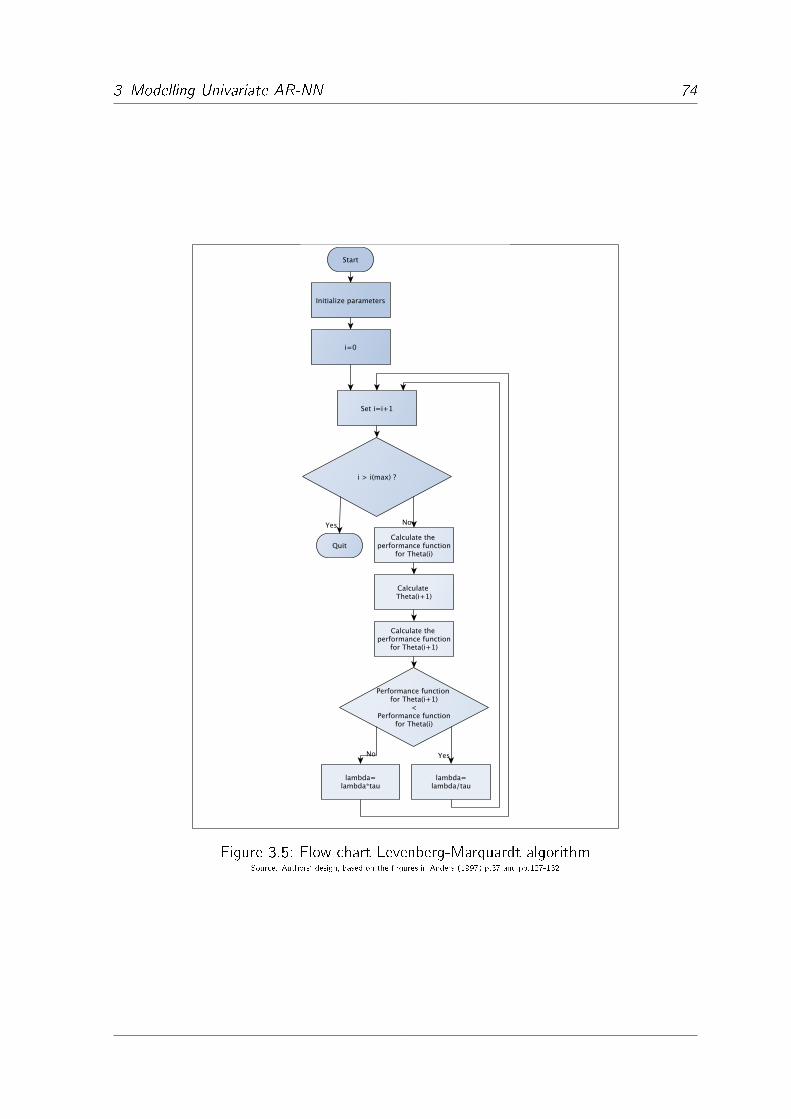
3 Modelling Univariate AR-NN 74
Figure 3.5: Flow chart Levenberg-Marquardt algorithmSource: Authors' design, based on the �rgures in Anders (1997) p.37 and pp.127-132
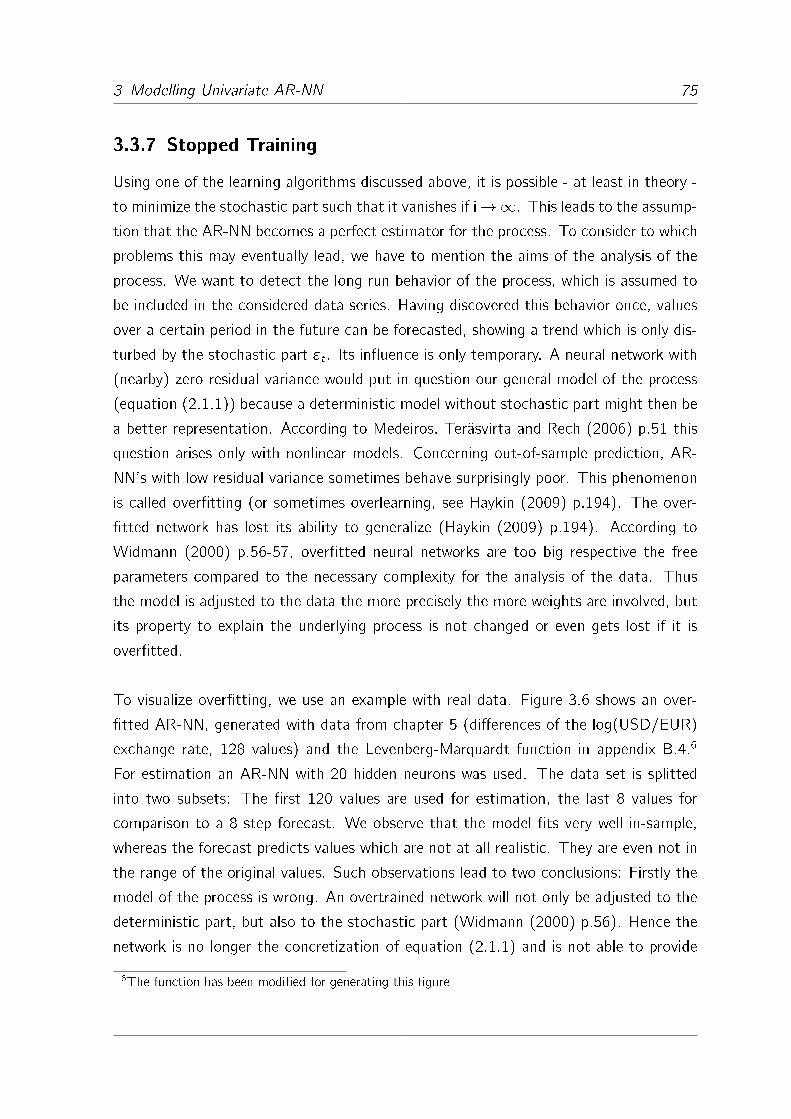
3 Modelling Univariate AR-NN 75
3.3.7 Stopped Training
Using one of the learning algorithms discussed above, it is possible - at least in theory -
to minimize the stochastic part such that it vanishes if i!1. This leads to the assump-
tion that the AR-NN becomes a perfect estimator for the process. To consider to which
problems this may eventually lead, we have to mention the aims of the analysis of the
process. We want to detect the long run behavior of the process, which is assumed to
be included in the considered data series. Having discovered this behavior once, values
over a certain period in the future can be forecasted, showing a trend which is only dis-
turbed by the stochastic part "t . Its in�uence is only temporary. A neural network with
(nearby) zero residual variance would put in question our general model of the process
(equation (2.1.1)) because a deterministic model without stochastic part might then be
a better representation. According to Medeiros, Teräsvirta and Rech (2006) p.51 this
question arises only with nonlinear models. Concerning out-of-sample prediction, AR-
NN's with low residual variance sometimes behave surprisingly poor. This phenomenon
is called over�tting (or sometimes overlearning, see Haykin (2009) p.194). The over-
�tted network has lost its ability to generalize (Haykin (2009) p.194). According to
Widmann (2000) p.56-57, over�tted neural networks are too big respective the free
parameters compared to the necessary complexity for the analysis of the data. Thus
the model is adjusted to the data the more precisely the more weights are involved, but
its property to explain the underlying process is not changed or even gets lost if it is
over�tted.
To visualize over�tting, we use an example with real data. Figure 3.6 shows an over-
�tted AR-NN, generated with data from chapter 5 (di�erences of the log(USD/EUR)
exchange rate, 128 values) and the Levenberg-Marquardt function in appendix B.4.6
For estimation an AR-NN with 20 hidden neurons was used. The data set is splitted
into two subsets: The �rst 120 values are used for estimation, the last 8 values for
comparison to a 8 step forecast. We observe that the model �ts very well in-sample,
whereas the forecast predicts values which are not at all realistic. They are even not in
the range of the original values. Such observations lead to two conclusions: Firstly the
model of the process is wrong. An overtrained network will not only be adjusted to the
deterministic part, but also to the stochastic part (Widmann (2000) p.56). Hence the
network is no longer the concretization of equation (2.1.1) and is not able to provide
6The function has been modi�ed for generating this �gure
3 Modelling Univariate AR-NN 76
Time
2000 2002 2004 2006 2008 2010
-0.10
-0.05
0.00
0.05
Original valuesFitted model8 step forecast
Figure 3.6: Example: Over�tted AR-NNSource: Authors' design
the expectation of this equation. The stochastic part is therefore an essential part of
the equation, which describes the dynamics of the process. The second conclusion is:
We need some stopping conditions which prevent the learning algorithm from adjusting
to the stochastic part.
A well known approach to solve the problem of over�tting is stopped training or early
stopping. The data set used for estimation is partitioned in an estimation subset (ES)
and a validation subset (VS). According to Haykin (2009) pp.202-203 in general an
estimation subset containing 80% of the values and a validation subset containing the
remaining 20% is a good partition. For alternative ways on how to partition the data see
the referred literature. If the model should be used for prediction, empirical application
shows that the validation subset should be as large as the number of steps to predict
(for example if the model is used for a 8 step forecast, the validation subset should
contain about 8 values). In our empirical part we observe that the AR-NN perform very
well in the short run (1-step or 2-step) forecasts. Consequently the validation subset
should be correspondingly small.
According to the stopped training method after each iteration the resulting parame-
ters are used to forecast the values of the validation subset. Subsequently the sum of

3 Modelling Univariate AR-NN 77
squares of the deviations of the forecasted from the original validation subset values
is calculated (in the following referred as VS-RSS). It is observable that the VS-RSS
is only minimized up to a �nite optimal number of iterations i*. If more iterations are
used, the VS-RSS will increase. The ES-RSS in contrast always decreases with increas-
ing number of iterations. Figure 3.7 shows a sketch how ES-RSS and VS-RSS develop
during the iterations.
i
RSSVS-RSS
ES-RSS
Minimum VS-RSS
i*
Figure 3.7: Stopped training: Development of ES-RSS and VS-RSS during the learning
algorithmSource: Authors' design, based on Bishop (1995) p.364 �gure 9.16
The parameter vector at the iteration where the VS-RSS is minimal (i*) is considered
to be the optimal parameter vector. Empirical application shows that an AR-NN with
a parameter vector chosen by the stopped training method is able to produce forecasts
which are at least in the range of the original values.
In application it is sometimes observable, that the results of the Levenberg-Marquart
algorithm depend on the initial values for the parameter vector. Stopped training pro-
vides a simple way to overcome this problem: The search for the minimum VS-RSS
does not start until some initial iterations are executed (in the empirical part for example
�ve initial iterations are used). In this way the initial values are modi�ed by the �rst
iterations in order to be more appropriate. In particular empirical application for this
dissertation showed that for such a procedure the di�erence in the results for various
initial values is lowered. Another fact that has been observed was that solutions at very
low numbers of iterations (iterations<5) often do not perform very well in out-of-sample
prediction.

3 Modelling Univariate AR-NN 78
Stopped training is just a method of limiting the iterative parameter estimation process
and not yet a solution for the problem of potentially too many hidden neurons. The
general approach to that problem is �nding the simplest model from a set of models
with the same goodness of �t the simplest model (Bishop (1995) p.14). Similar to linear
time series analysis it is possible to check wheater the in�uence of certain parameters is
signi�cant for the model. Further if only the �rst (1+ n) parameters were su�cient for
the model, a linear model would be a better approach. Therefore such tests are some-
times referred to as linearity tests, see section 3.1. Of course there are some ex-ante
parameter determination methods (for example the rule Baum and Haussler (1988)),
but they are not so powerful as the ex-post parameter tests for they are not built on
a sound theoretical fundament like parameter hypothesis tests. Therefore we abstain
from explaining them (for an overview see Widmann (2000) pp.57-65) and recommend
the testing procedures discussed in the following sections.
3.4 Parameter Tests
The �nal step is now to examine if the estimated model is appropriate. This can be
performed in two ways:7 Bottom-up means starting with the estimated model. It is
examined, if an additional hidden unit would improve the model. Therefore the non-
linearity test already known from section 3.1 is extended. Their disadvantage is, that
they only consider the in-sample performance (for example the in-sample RSS) of the
models. An alternative is cross validation, which means that the quality of a model is
evaluated by its out-of-sample performance.
Top-down parameter tests are well known from linear statistics. They consider one
parameter or a set of parameters within the estimated model and test them on signif-
icance. For an estimated model the general procedure is �rst to execute bottom-up
parameter tests as long as no additional hidden unit improves the model. Then a model
including those additional hidden units is again estimated and evaluated by top-down
parameter tests (see �gure 3.1 for an overview how top-down and bottom-up parameter
tests are used).
7The notations bottom-up and top-down parameter testing are taken from Anders (1997) pp.127-128
3 Modelling Univariate AR-NN 79
3.4.1 Bottom-Up Parameter Tests
In this section two methods for bottom-up evaluation of an estimated model are dis-
cussed. The �rst method is based on Taylor polynomial estimation of an additional
hidden neuron. Therefore the test of Lee, White and Granger (1993) (see also section
3.1.2.2) is slightly modi�ed by Teräsvirta, Lin and Granger (1993). As this test only
examines the in-sample contribution of an additional hidden unit, a second procedure
is proposed: Cross-validation, an approach similar to stopped training, considers the
out-of-sample contribution of the additional hidden unit.
3.4.1.1 The Test of Lee, White and Granger
The test of Lee, White and Granger (1993), related to the test of Teräsvirta, Lin and
Granger (1993), can also be used as a test on additional hidden nonlinearity. Equation
(3.1.9) includes here an AR-NN G(�; Xt�1)
xt = G(�; Xt�1) + ut ; (3.4.1)
with
ut = (F (Xt�1)� G(�; Xt�1)) + "t : (3.4.2)
If the �rst term in equation (3.4.2) is zero, the estimated AR-NN G(�; Xt�1) does
explain the process completely and there is no additional hidden nonlinearity. To test this
like in equation (3.1.12) an additional hidden neuron is added to the AR-NN equation:
xt = G(�; Xt�1) + ( 0a + �>a Xt�1)�a + "t (3.4.3)
The index a indicates the additional hidden neuron. The further procedure is now the
same as in the nonlinearity test. The arti�cial linear regression of equation (3.1.17)
becomes
ut = �1rG(�; Xt�1) + �2(( 0a + �>a Xt�1)) + u�t : (3.4.4)
The second term of this equation is approximated by a Taylor polynomial, such that
equation (3.4.4) becomes for the tanh activation function (like equation (3.1.20)):
ut = �1rG(�; Xt�1)� 1
3
n∑j1=1
n∑j2=j1
n∑j3=j2
�2j1;j2;j3xj1xj2xj3 + u�t (3.4.5)
3 Modelling Univariate AR-NN 80
Thus the null hypothesis can be written as
H0 : �2j1;j2;j3= 0 8 j1; j2; j3 (3.4.6)
with alternative
H1 : �2j1;j2;j36= 0 8 j1; j2; j3: (3.4.7)
The calculation of the test statistics is the same as in subsection 3.1.2.1 (equations
(3.1.18) and (3.1.19)). The only di�erence is the second degree of freedom for the F
test statistic, which is here (T � r).
3.4.1.2 Cross Validation
The formal LM test mentioned in the previous subsection only checks if one additional
hidden neuron can improve the in-sample performance of a model. But in the empir-
ical part of this dissertation (especially tables 5.10 to 5.13) the main focus is on the
out-of-sample performance of AR-NN. It does not always behave in a parallel way to
the in-sample performance. Therefore an intuitive method which considers the out-of-
sample behavior of the models can be used as an alternative to the formal bottom-up
parameter tests (see for example Inoue and Kilian (2006) p.273 for this idea).
The procedure is similar to the one shown in section 3.3.7. The data set is split-
ted into a training subset (at which for example stopped training may be applied) and
a so called test subset (see Haykin (2009) p.201). Cross validation is executed in three
steps:
� In the �rst step several models with increasing h - starting with h=0 - are adjusted
to the training subset.
� In the second step the values of the test subset are predicted out of the estimated
models. Those values are compared to the original values of the test subset (for
example by calculating the RMSE between estimated and original values).
� The model with the lowest test subset RMSE is the optimal model. If the test
subset RMSE does not di�er signi�cantly for some models, the model with the
lowest h (and thus the smallest number of parameters) should be chosen.
3 Modelling Univariate AR-NN 81
3.4.2 Top-Down Parameter Tests
The principle of top-down parameter testing is well known in statistics.The aim of such
procedures is to check in an already estimated model if all or certain parameters are
signi�cant. Hence the notation top-down describes to start with the estimated model
and check if not a smaller model (according to the Occam's razor principle) is better.
In this section we propose two types of parameter tests for AR-NN. Those procedures
can also be applied at other forms of nonlinear functions (as Taylor-polynomials for
example). The �rst type is an IC. The Neural Network IC (NIC) is a generalization of
the AIC and has therefore to be minimized like the AIC. We use this method in accor-
dance to the authors of the original paper (Murata, Yoshizawa and Amari (1994)) to
detect the optimal number of hidden neurons. Using the AIC itself would lead to mis-
speci�cations. Murata, Yoshizawa and Amari (1994) p.876 cite a japanese study which
shows that problems occur if certain models with di�erent numbers of hidden neurons
are compared. Alternatively the NIC can be used to detect the number of input neurons
or lags, see Anders (1997) p.77. Then the NIC would belong to section 5.4.1. Another
possible alternative would be to vary lags and hidden neurons simultaneously to detect
an optimal combination of lags and hidden neurons.
The second type of methods discussed in this section for testing the signi�cance of
parameters is one of the the classical parameter hypothesis testing procedures in sta-
tistical models: The Wald test. The additional feature of this test is the possibility to
examine each single (as well as �)-weight for signi�cance. Anders (1997) pp.64-73
also mentions the other classical parameter tests, the likelihood ratio (LR) test and the
LM test, in context with neural networks, but there are sone arguments which speak
against them:
The LR test examines two separately estimated models against each other (a restricted
and a unrestricted model). This makes only sense if the parameters are estimated by the
same algorithm. If a numerical algorithm in combination with stopped training is used,
the two models may react di�erently on the algorithm. Thus here we would compare
two di�erently estimated models, which does not make any sense for the LR test.
Using the LM test as a top-down parameter test means splitting the AR-NN into two
parts (the one contains the hidden neurons which should be examined, the other con-

3 Modelling Univariate AR-NN 82
tains the rest) to execute the arti�cial linear regression with both parts. In particular if
the number of hidden units is large, splitting o� one or more of them o� will lead into
a huge programming e�ort, which is not justi�ed as the Wald test or the NIC examine
the same hypothesis and are simpler to implement.
3.4.2.1 Consistency
A prerequisite for parameter tests is the existence of a distribution of the estimated
weights, which can be determined at least asymptotical. This requires that the esti-
mators are consistent, which means that they converge to their true value if T ! 1(see Anders (1997) p.57). Once consistency of the estimators has been shown it is
possible to prove with the help of the central limit theorem the multivariate Gaussian
distribution of a standardization of � for a su�cient large T (see Widmann (2000)
p.53). This distribution is necessary for parameter tests.
A prerequisite of consistency for parameter estimators is that the "true" value of the
parameter vector is identi�ed, which means that there exists a unique minimum (not
necessarily the global minimum) of the performance function. Particularly for neural
networks it might be possible that two di�erent network structures lead to the same
minimum. Hence it is absolutely necessary to prespecify the number of hidden neurons
h and lags n appropriately, such that no unnecessary parameters are involved (see Wid-
mann (2000) p.54). The lag selection methods as well as the selection of h such that
the relation T=r is about 10% might be helpful to avoid overparametrization. Another
problem is the order of the hidden units. For any estimated AR-NN with more than one
hidden unit the same performance result can be achieved if the order of the hidden units
is exchanged. Therefore always two di�erent parameter vectors exist for each minimum.
In addition some restrictions or conditions are necessary to guarantee the uniqueness
of an optimal parameter vector. The results of White and Domowitz (1984) on the
consistency of AR-NN parameters can be recapitulated in the following according to
time series speci�c version of Trapletti, Leisch and Hornik (2000) pp.2431-2434. At
�rst some conditions have to be de�ned and explained:
Condition 3.1 (Trapletti, Leisch and Hornik (2000) p.2432 assumption 1):
Each hidden neuron contributes nontrivial to the process such that
3 Modelling Univariate AR-NN 83
( 0j + �>j Xt�1) 6= 0 and �j 6= 0. All inputs of the hidden neurons are not sign
equivalent such that j 0j + �>j Xt�1j 6= j 0k + �>k Xt�1j 8j; k = 1; : : : ; h.
This condition should ensure that it is not possible to archive the same equation with
fewer hidden units, i.e. that no unnecessary hidden neurons are included. The second
part of this condition in particular excludes the twofold existence (with di�erent presign)
of any hidden neuron.
Condition 3.2 (Trapletti, Leisch and Hornik (2000) p.2433 assumption 2):
The data generating process is a stationary AR-NN with continuos activation function
and the weight space � � Rr .
This condition restricts the weight space � such that all roots of the characteristic
polynomial of the linear part are outside the unit circle (see theorem 2.2). The other
weights are restricted to be real numbers.
Condition 3.3 (Trapletti, Leisch and Hornik (2000) p.2434 assumption 3):
�j > 0 8j = 1; : : : ; h and �j < �j+1 8j = 1; : : : ; h � 1.
This condition avoids the problem of changing the order of the hidden units as we have
discussed before. The restriction of all �j on positive numbers rules out the possibility
of reaching the same value by changing the - and �-weight signs. Conditions 1 to 3
restrict the set of possible solutions such that a unique minimum exists for certain ac-
tivation functions. Those activation functions have to archive the following condition:
Condition 3.4 (Trapletti, Leisch and Hornik (2000) p.2434 assumption 4):
All functions ( 0k +�>j Xt�1) and the constant 1 are linear independent 8j = 1; : : : ; h
and any Xt�1 � Rn.
The tanh activation function ful�lls in general this condition.8 Theorem 3.1 in the
8But if the input is large and always positive/negative, then it would in fact become a constant on the
upper bound of its range of values. This is not a realistic case because already in theorem 2.1 it was
stated that the weight space should contain a neighbourhood of the origin.

3 Modelling Univariate AR-NN 84
following shows how a NLS-estimator � is consistent:
Theorem 3.1 (Trapletti, Leisch and Hornik (2000) p.2434 theorem 5):
If conditions 1-4 are achieved and Ej"2t jk < 1 for any k > 1, the NLS estimator �
converges almost sure (a.s.) to the true parameter vector �, �a:s:��! �.
PROOF: For the proof see Trapletti, Leisch and Hornik (2000) p.2439.
Two additional conditions are necessary to calculate the asymptotic normal standard-
ized distribution of �:
Condition 3.5 (Trapletti, Leisch and Hornik (2000) p.2434 assumption 5):
The original weight vector � is in � and (�) is continuously di�erentiable of order 2.
Condition 3.6 (Trapletti, Leisch and Hornik (2000) p.2434 assumption 6):
All 0( 0j +�>j Xt�1), Xt�10( 0j +�>j Xt�1) and the constant 1 are linear independent
8j = 1; : : : ; h and any Xt�1 � Rn.
The tanh activation function satis�es condition 5 and 6. Condition 1 and 6 together
ensure the regularity of the information matrix at �. Theorem 3.2 shows the standard-
ized distribution of �:
Theorem 3.2 (Trapletti, Leisch and Hornik (2000) p.2434 theorem 6):
If all conditions are achieved, Ej"3t jk <1 for any k > 1 and T !1, then
1
�
√r2Q(�) � (���)
d�! N(0; Ir); (3.4.8)
whereasd�! denotes convergence in distribution.
PROOF: For the proof see Trapletti, Leisch and Hornik (2000) p.2439
Ir denotes the r dimensional identity matrix. This result is the basis for the hypothesis

3 Modelling Univariate AR-NN 85
tests in the following section. An alternative representation of equation (3.4.8) using
the (r � r) dimensional covariance matrix C of the parameters, is
pT (���)
d�! N(0;C): (3.4.9)
An estimator C for C can be received by
C = ��1���1; (3.4.10)
using the crossproduct of the gradient vectors multiplied by T�1
� =1
T(rQ(�))>(rQ(�)) (3.4.11)
and the Hessian matrix multiplied by T�1
� =1
Tr2Q(�) (3.4.12)
see Murata, Yoshizawa and Amari (1994) p.173 and Onoda (1995) p.278. The relation
between the equations (3.4.8) and (3.4.9) is as follows: If the model is appropriate, the
crossproduct of the gradient vectors should be equal to the Hessian matrix,
� = �2�: (3.4.13)
Consequently equation (3.4.10) is reduced to
C = �2��1; (3.4.14)
see White and Domowitz (1984) p.152. Therefore equation (3.4.8) is the usual trans-
formation of equation (3.4.9) to a standard Gaussian distribution:
pT (���)
d�! N(0;C)
C� 1
2
pT (���)
d�! N(0; Ir)1
�
p�T (���)
d�! N(0; Ir)
(3.4.15)

3 Modelling Univariate AR-NN 86
3.4.2.2 The Neural Network Information Criterion
The Neural Network Information Criterion (NIC) is a generalization of the AIC to de-
tect nonsigni�cant components. It is especially designed for misspeci�ed models, where
the usual AIC or BIC can not be used (see Anders (1997) p.77). The AIC in time
series analysis is rather used for lag selection than for parameter tests. Hence it is of
course possible to use its generalized equivalent, the NIC, also for such aims. Yet this
would imply estimating several AR-NN models ex-ante which requires much more e�ort
than to approximate them via the methods of section 3.2 (Taylor polynomials, kernel
regression etc.).
First some notations for di�erent AR-NN models have to be introduced. Suggest k neu-
ral network functions for the same time series are given, G1(�1; Xt�1), G2(�2; Xt�1),
: : :, Gh(�h; Xt�1). Let �1 2 Rr1, �2 2 Rr2, : : :, �h 2 Rrh for r1 < r2 < : : : < rh. h indi-
cates the originally introduced number of hidden neurons. This means that the number
of hidden neurons in the second function is lager than that in the �rst function and
so on. The di�erent models Gj(�j ; Xt�1), j = 1; : : : ; h are not estimated separately.
Rather we use the estimated � � � and delete descending from the largest model
Gh(�h; Xt�1) the part of the equation as well as the elements of � which correspond
to the hidden neuron which is not contained in the lower model. Thus we can say that
the functions are nested submodels,
G1(�1; Xt�1) � G2(�2; Xt�1) � : : : � Gh(�h; Xt�1): (3.4.16)
Instead of the discrepancy functions proposed in Murata, Yoshizawa and Amari (1994)
pp.870-871 we use for each model j the performance function
Q(�j) =1
2
T∑i=1
(xt � Gj(�j ; Xt�1))2 (3.4.17)
known from section 3.3.1. The NIC is de�ned for model j using �j and �j by
NICj =1
T
(1
2
T∑t=1
"2jt + tr(�j��1j )
): (3.4.18)
The second term is called penalty term because it "punishes" the excessive usage of
parameters. Should the model j be faithful, which means that �j is a (optimal) NLS
3 Modelling Univariate AR-NN 87
solution, we know from equation (3.4.13) that �j = �2j �j . A consequence would be
that
tr(�j��1j ) = �2 � tr(I) = �2r (3.4.19)
Thus in this case the NIC is equal to the AIC2 (equation (3.2.2)). Like any other IC
the NIC has to be minimized, thus we choose the submodel with the lowest NIC.
The NIC, like any other IC, is not consistent. If IC in general are used as parameter
tests, it has to be ensured that no irrelevant hidden neurons are included in the models
(see Anders (1997) p.78). If the models are overparametrized, �j and �j are degener-
ated and may diverge heavily. The consequence is an unusual large NIC value. Hence
large NIC's can be interpreted as an sign for overparametrization (see Anders (1997)
p.79).
3.4.2.3 The Wald Test
Before the Wald test (rooted in Wald (1943)) can be executed, it is necessary to
estimate the covariance matrix C using equation (3.4.10). In addition no irrelevant
hidden neurons should be included in the models. For the following see Widmann (2000)
pp.100-102 and Anders (1997) pp. 72-73. The simplest application of the Wald test
is to consider a null hypothesis of non-signi�cance for each single weight,
H0 : �i = 0 8 i = 1; : : : ; r: (3.4.20)
In this case the test statistic is
TWALD1=
�2i�2�i
: (3.4.21)
The denominator �2�iis the variance of �i . This equals the ith element on the principal
diagonal of C. The test statistic is �2 distributed with one degree of freedom (see An-
ders (1997) p.73). Davidson and MacKinnon (1993) p.89 call it "pseudo- t-statistic".
4 Multivariate models 88
4 Multivariate models
4.1 Multivariate AR-NN
4.1.1 Vector Autoregressive Neural Network Equations
Our knowledge of neural network modelling of autoregressive processes now is easily
extendable to nonlinear vector autoregressive models. In general multivariate modelling
means to add an additional dimension - the number of variables m - to a univariate
model. The idea of multivariate AR-NN is based on Raman and Sunlikumar (1995)
and Chakraborty et al. (1992), although vector representation as we will use it in this
section is not treated by those authors. A vector autoregressive process is introduced
formally (equivalent to de�nition 2.1) by
De�nition 4.1 (Vector autoregressive process (VAR)):
A process is called vector autoregressive process of order n - short VAR(n) - if it is
described by the functional relation
Yt = F (Yt�1) + Et ; (4.1.1)
whereas Yt = (y1t ; y2t ; : : : ; ymt) is a vector of m variables and Yt�1 is a (m � n � 1)
vector of the lagged variables,
Yt�1 = (Yt�1; Yt�2; : : : ; Yt�n)> (4.1.2)
with F : Rmn ! Rm and Et = ("1t ; "2t ; : : : ; "mt)> is a m-dimensional Gaussian dis-
tributed WN vector.
Remark 4.1.1:
If F (Yt�1) is a linear function, the process is a linear VAR. If F (Yt�1) is nonlinear it is
a nonlinear VAR.

4 Multivariate models 89
A linear VAR is represented by
Yt = A0 + A1Yt�1 + A2Yt�2 + : : :+ AnYt�n + Et (4.1.3)
whereas the constant matrix A0 has dimension (m � 1)and the parameter matrices Ai
8 i = 1; : : : ; n have dimension (m � m) . An alternative representation of equation
(4.1.3) is
Yt = A0 + A︸︷︷︸(m�m�n)
Yt�1︸︷︷︸(m�n�1)
+Et ; (4.1.4)
whereas A = (A1; A2; : : : ; An). In full matrix representation equation (4.1.4) is written
as follows: y1;t
y2;t...
ym;t
=
�01
�02
...
�0m
+
�111 : : : �11m : : : �n1m
�121 : : : �12m : : : �n2m
......
......
...
�1m1 : : : �1mm : : : �nmm
y1;t�1
...
y1;t�n...
y2;t�1
...
ym;t�n
+
"1t...
"mt
By the independence assumptions of the residuals one can divide (4.1.4) into m inde-
pendent linear equations
yj;t = �0j + �1j1y1;t�1 + : : :+ �1jmym;t�1 + �2j1y1;t�2 + : : :+ �njmym;t�n + "jt (4.1.5)
for each variable j = 1; : : : ; m. The separate models for each output neuron have the
same dimensional properties like univariate models. The main di�erence is, that there
are some additional variables which might be Granger-causal to the output variable.
Informally in times series context a variable y2 is said to Granger-cause any other variable
y1, if its lagged past values signi�cantly contribute to explain the present state of y1
4 Multivariate models 90
(see for example Granger (1988) p.203). The neural network modelling procedure
discussed here is equivalent to a linear VAR like equation (4.1.3). In particular the
property to split the multivariate model into several independent univariate models (like
in equation (4.1.5)) is essential. Let us introduce the following additional matrix terms
for formulation of the Vector AR-NN (VAR-NN):
�0;j =
0j1
0j2...
0jm
�i ;j =
i j11 i j12 : : : i j1m
i j21 i j22 : : : i j2m...
......
...
i jm1 i jm2 : : : i jmm
�j = (�1j ; �2j ; : : : ; �nj)
(4.1.6)
A VAR-NN is thus de�ned by the multivariate version of equation (2.2.7):
Yt︸︷︷︸(m�1)
= A0︸︷︷︸(m�1)
+ A︸︷︷︸(m�mn)
Yt�1︸︷︷︸(mn�1)
+
h∑j=1
( �0j︸︷︷︸(m�1)
+ �j︸︷︷︸(m�mn)
Yt�1︸︷︷︸(mn�1)
) �j︸︷︷︸1�1
+ Et︸︷︷︸m�1
(4.1.7)
In this case : Rm ! Rm whereas each element is transformed individually by the
activation function (the tanh for example). Like in the linear case (equation (4.1.5)),
m independent models can be splitted o�. Note that the parameter �j is scalar (1� 1)
to keep the structure of the NN-VAR straightforward. In addition �j has to be prespec-
i�ed, because it can not be estimated simultneaously with the other parameters.
Stopped training becomes more complicated in the multivariate models, as for esti-
mation the equations have to be separated, but for forecasting they have to be added
together. The problem is, that for forecasting one variable, one also needs the estimated
4 Multivariate models 91
models for the other variables. One may proceed as follows: Firstly the parameter vec-
tors are estimated for each variable and saved for each iteration. Then the multivariate
model is used to evaluate all combinations of the parameters in each iteration. The
optimal model minimizes the VS-RSS for each variable. Such a procedure requires much
e�ort, especially for implementing all the combinations of parameter vectors. Hence we
recommend to abstain from stopped training in the multivariate models.
One has to overcome a di�culty if the lag selection methods from section 3.2 are
applied at VAR-NN. The lag selection methods can be applied at the submodels of the
VAR-NN without problems but the result are certainly di�erent lag structures. Merging
the submodels to a VAR-NN is then impossible. Thus a procedure has to be imple-
mented which detects the optimal lag for the whole AR-NN. The following steps might
provide a solution:
� Calculate the lag selection criterion for several lags for the submodels (especially
for the methods in 3.2.3 and 3.2.4 the submodels can be approximated by Taylor
expansion or local linear estimation as well as the univariate models).
� Sum the lag selection criteria of all submodels for each lag.
� Choose that lag where the sum of lag selection criteria is minimal.
The last step results of the fact that the lag selection criteria in general have to be
minimized. The parameter estimation methods may in a similar way also be used simul-
taneously for the submodels. But they also allow for partly weakly exogeneity of some
variables if parts of the multivariate hidden neurons are not signi�cant. Alternatively
the lag order can be detected by the average lag of the univariate time series optimal
lag orders.
4.1.2 Vector Autoregressive Neural Network Graphs
To start with graph representation of a VAR-NN, we �rst consider the graph of a linear
VAR(2) with two variables using the symbols from section 2.2.1 with white circles for
the �rst variable and yellow circles for the second variable (see �gure 4.1). The output
neurons in this graph can be considered separately (see �gure 4.2 for the separated
�rst variable). In the following we draw the graph of a VAR-NN(2) with two variables.
Before we proceed with the multivariate AR-NN we have to introduce some additional
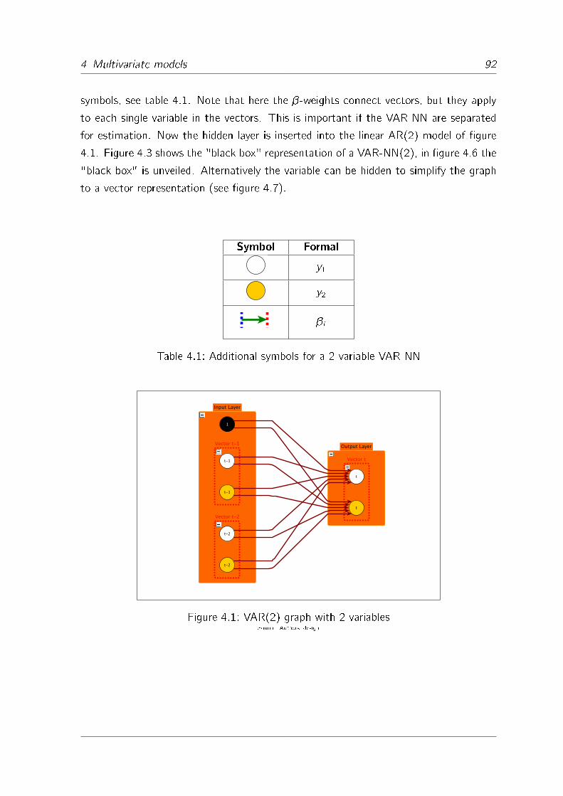
4 Multivariate models 92
symbols, see table 4.1. Note that here the �-weights connect vectors, but they apply
to each single variable in the vectors. This is important if the VAR-NN are separated
for estimation. Now the hidden layer is inserted into the linear AR(2) model of �gure
4.1. Figure 4.3 shows the "black box" representation of a VAR-NN(2), in �gure 4.6 the
"black box" is unveiled. Alternatively the variable can be hidden to simplify the graph
to a vector representation (see �gure 4.7).
Symbol Formal
y1
y2
�i
Table 4.1: Additional symbols for a 2 variable VAR-NN
Figure 4.1: VAR(2) graph with 2 variablesSource: Authors' design

4 Multivariate models 93
Figure 4.2: Separated model of the �rst variableSource: Authors' design
Figure 4.3: VAR-NN(2) - "black box" representationSource: Authors' design

4 Multivariate models 94
Figure 4.4: VAR-NN(2) graphSource: Authors' design
Figure 4.5: VAR-NN(2) - vector representationSource: Authors' design
4 Multivariate models 95
4.2 Neural Networks and Cointegration
The concept of cointegration has become essential in time series analysis since Engle
and Granger (1987). In general the term cointegration is de�ned by (see for example
Johansen (1995) p.35):
De�nition 4.2 (Cointegration):
If for a vector Yt of m series of the same integration order � 1 a stationary linear
combination B>Yt , exists, the series are called cointegrated with cointegration matrix
B of dimension (c �m) with c < m. If c=1, B is called cointegration vector.
In this section we will show how cointegration can be related to our AR-NN models.
Note that this section is not about nonlinear cointegration but rather about nonlin-
ear adjustment in vector error-correction models (VEC), see therefore Dufrenot and
Mignon (2002) p.224.
4.2.1 Nonlinear Adjustment in Error Correction Models
First of all we consider a linear VEC in reduced rank representation as for example in
Johansen (1995) p.45:
�Yt = KB>Yt�1 + A0 + A1�Yt�1 + : : :+ �Yt�n + Et (4.2.1)
B is the (m � c) cointegration matrix with 0 6= c < m and K is the (m � c) loading
matrix. c is the number of cointegration relationships. For details see Johansen (1995)
pp.45-69. The cointegration matrix in�uences the variables via K through a linear
relationship. If there is nonlinearity in the data, nonlinear instead of linear adjustment
might improve the model (4.2.1). Using the nonlinear function F (�) equation (4.2.1)
can be rewritten as
�Yt = F(B>Yt�1
)+ A0 + A1�Yt�1 + : : :+ �Yt�n + Et : (4.2.2)

4 Multivariate models 96
Note that here F : Rc ! Rm is the nonlinear equivalent to K in equation (4.2.1). This
VEC can be illustrated by a simple bivariate example from Escribano and Mira (2002)
p.514:
�xt = �11�xt�1 + f1(zt�1) + v1t (4.2.3)
�yt = �21�yt�1 + f2(zt�1) + v2t (4.2.4)
zt = xt � byt (4.2.5)
zt is the cointegration relationship and the cointegration vector here is B = (1; b)>.
f1(�) and f2(�) are nonlinear functions mapping F1; F2 : R ! R, Yt = (xt ; yt)>,
F (B>Yt�1) =
(f1(zt�1)
f2(zt�1)
)(4.2.6)
and
A =
(�11 0
�21 0
)(4.2.7)
4.2.1.1 Theoretical Prerequisites
Now should be shown how such a nonlinear VEC is theoretically justi�ed. We will there-
fore use theorem 3.7 in Escribano and Mira (2002) p.517. For the formulation two new
expressions have to be introduced, which both are closely related to stationarity: �-
mixing and near epoch dependency (NED). With those constructs a functional central
limit theorem holds for the nonlinear error correction theorem. Such a functional central
limit theorem is the basis for estimation and inference (see Escribano and Mira (2002)
p.511-512). For this section see Escribano and Mira (2002) pp.512-515.
Beforehand some mathematical notations have to be explained: Let be the set of all
possible realizations of a process xt . The �-algebra F of is then de�ned as a system
of subsets which
4 Multivariate models 97
� contains the null set
� contains for each subset A 2 F also the complement �A of A
� contains for a (possibly) in�nite (i ! 1) sequence of sets Ai also their union⋃i Ai
see Hassler (2007) p.14. The �-algebra F ts = �(xs ; : : : ; xt) generated by a process xt
is de�ned as the smallest �-algebra for which xt is measurable. Therewith the mixing
coe�cients � are de�ned as
�k = supt
supfF12F t
�1;F22F1t+k
gjP rob(F1F2)� P rob(F1)P rob(F2)j (4.2.8)
sup denotes the supremum (upper bound) of a set. We call the process �- or strong-
mixing if �k ! 0 as k !1. A strong- mixing process can be interpreted as a process,
where the dependence between two realizations of the process xt , which are separated
by k steps, decreases as k increases. The mixing coe�cient �k measures this depen-
dence. A stationary process is strongly mixing (but not vice versa).
The second concept necessary for the nonlinear error correction theorem is the NED.
Let yt be a process with a �nite sum of squares (E(y 2t ) < 1). yt is NED of size �a
on the process xt if
�(n) = supt
= jjyt � E(yt jxt�n; : : : ; xt+n)jj2 (4.2.9)
is of size �a. jj � jj2 is the L2-norm E1
2 j � j2. To keep this concept in accordance with AR
theory, we assume that the forward values of xt , xt+i 8 i = 1; : : : ; n do not improve the
conditional expectation and are therefore useless. If �(n) goes to zero as n increases,
it can be said that yt essentially depends on the recent epoch of xt . yt is NED of any
size if it depends on a �nite number of lags of xt .
The NED property is important to characterize an I(0)-process via a functional central
limit theorem for NED variables. The functional central limit theorem for NED pro-
cesses explains how a standardization of an I(0) NED process converges to a standard
Brownian motion and justi�es thus the distribution of such a process.
4 Multivariate models 98
Theorem 4.1 (Escribano and Mira (2002) p.513 theorem 2.3):
Let xt be a process with zero mean, uniformly Ls-bounded and NED of size �12on an
�-mixing process of size �s=(s � 2) and T�1E(∑T
t=1 xt)2 ! �2, �2 2]0;1[. Then
T� 1
2
∑[Ts]t=1 xt coverges to a standard Brownian motion B(s).
A process yt is I(0) if it is NED on a mixing process xt , but the process wt =∑t
s=1 ys
is not NED on xt . If wt =∑t
s=1 ys is NED on xt , the process is I(1). Similarly we can
express linear bivariate cointegration in terms of NED: Two I(1) processes xt and yt are
linearly cointegrated with cointegration vector B = (1;�b)> if xt � byt is NED on a
strong-mixing process, but xt��yt is not NED on a strong mixing process for any � 6= b.
In the following we will use the nonlinear VAR
Zt = H(Zt�1) + Ut (4.2.10)
with dimensions of Zt and Ut (c � 1). H(�) : Rc ! Rc is a di�erentiable function of a
variable Z on an open set of Rm. Under the following assumptions and conditions is Zt
NED on the �-mixing sequence Ut :
� Ut is �-mixing of size �s=(s � 2) for s > 2.
� SR(JZ(H(Z))) � 1 � �, whereas SR(�) denotes the spectral radius of a matrix,
which is its largest eigenvalue. JZ(H(Z)) denotes the Jacobi matrix of H(Z) with
respect to Z. Its dimension is (c � c). This condition is also called boundedness
condition, because it limits the largest eigenvalue of the Jacobian matrix away
from 1. The boundedness condition is a su�cient condition for H(Zt�1) to be
NED (see Escribano and Mira (2002) p.516).
� Let �u be a �nite constant and EjjUt jj2S = �u. jj � jjS denotes a subordinate matrix
norm.
4.2.1.2 The Nonlinear Error Correction Model and Neural Networks
Using the notations from the section above, we can formulate the VEC-theorem of
Escribano and Mira (2002) p.517. Note that the theorem is formulated for only one
lag (n = 1) in the VAR-part:
�Yt = A1�Yt�1 + F (B>Yt�1) + Et (4.2.11)
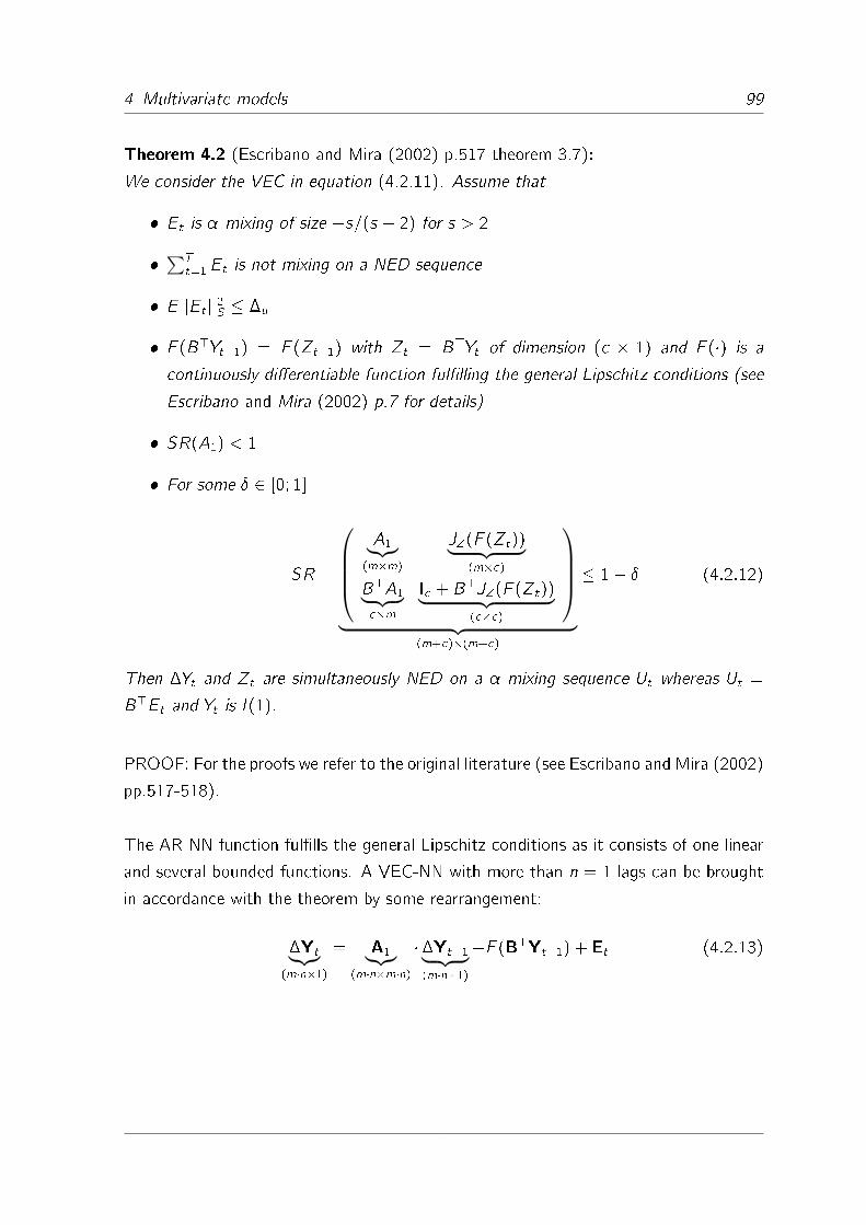
4 Multivariate models 99
Theorem 4.2 (Escribano and Mira (2002) p.517 theorem 3.7):
We consider the VEC in equation (4.2.11). Assume that
� Et is �-mixing of size �s=(s � 2) for s > 2
�
∑T
t=1 Et is not mixing on a NED sequence
� EjjEt jj2S � �u
� F (B>Yt�1) = F (Zt�1) with Zt = B>Yt of dimension (c � 1) and F (�) is a
continuously di�erentiable function ful�lling the general Lipschitz conditions (see
Escribano and Mira (2002) p.7 for details)
� SR(A1) < 1
� For some � 2 [0; 1]
SR =
A1︸︷︷︸
(m�m)
JZ(F (Zt))︸ ︷︷ ︸(m�c)
B>A1︸ ︷︷ ︸c�m
Ic + B>JZ(F (Zt))︸ ︷︷ ︸(c�c)
︸ ︷︷ ︸
(m+c)�(m+c)
� 1� � (4.2.12)
Then �Yt and Zt are simultaneously NED on a �-mixing sequence Ut whereas Ut =
B>Et and Yt is I(1).
PROOF: For the proofs we refer to the original literature (see Escribano and Mira (2002)
pp.517-518).
The AR-NN function ful�lls the general Lipschitz conditions as it consists of one linear
and several bounded functions. A VEC-NN with more than n = 1 lags can be brought
in accordance with the theorem by some rearrangement:
�Yt︸︷︷︸(m�n�1)
= A1︸︷︷︸(m�n�m�n)
��Yt�1︸ ︷︷ ︸(m�n�1)
+F (B>Yt�1) + Et (4.2.13)

4 Multivariate models 100
with Yt = (Yt ; : : : ; Yt�n)>, Yt�1 = (Yt�1; : : : ; Yt�n�1)>, B = (B; : : : ; B︸ ︷︷ ︸
n times
)>, F : Rr !
Rm�n, Et = (Et ; : : : ; Et�n)> and
A1 =
A1 : : : An
. . ....
. . .
A1 : : : An
However for estimation of the nonlinear VEC we may use the usual form (equation
4.2.2). We can formulate an example for a bivariate nonlinear VEC with an AR-NN
representation of F (Zt�1) and one cointegration relationship (c = 1). Let n = 1 and
h = 1 (see also Dufrenot and Mignon (2002) pp.229-243 for other applications of the
VEC of Escribano and Mira (2002)):
zt = yt � bxt (4.2.14)
�xt = ��11�xt�1 + ��12�yt�1 +
�01 + �11zt�1 +( 01 + 11zt�1)� + "1t (4.2.15)
�yt = ��12�yt�1 + ��22�xt�1 +
�02 + �12zt�1 +( 02 + 12zt�1)� + "2t (4.2.16)
A vector representation of equations (4.2.14), (4.2.15) and (4.2.16) together is given
in the following:(�xt
�yt
)=
(��11 �
�12
��21 �
�22
)(�xt�1
�yt�1
)+(
�01
�02
)+
(�11
�21
)zt�1 +
(( 01
02
)+
( 11
11
)zt�1
)�
+
("1t
"2t
)(4.2.17)
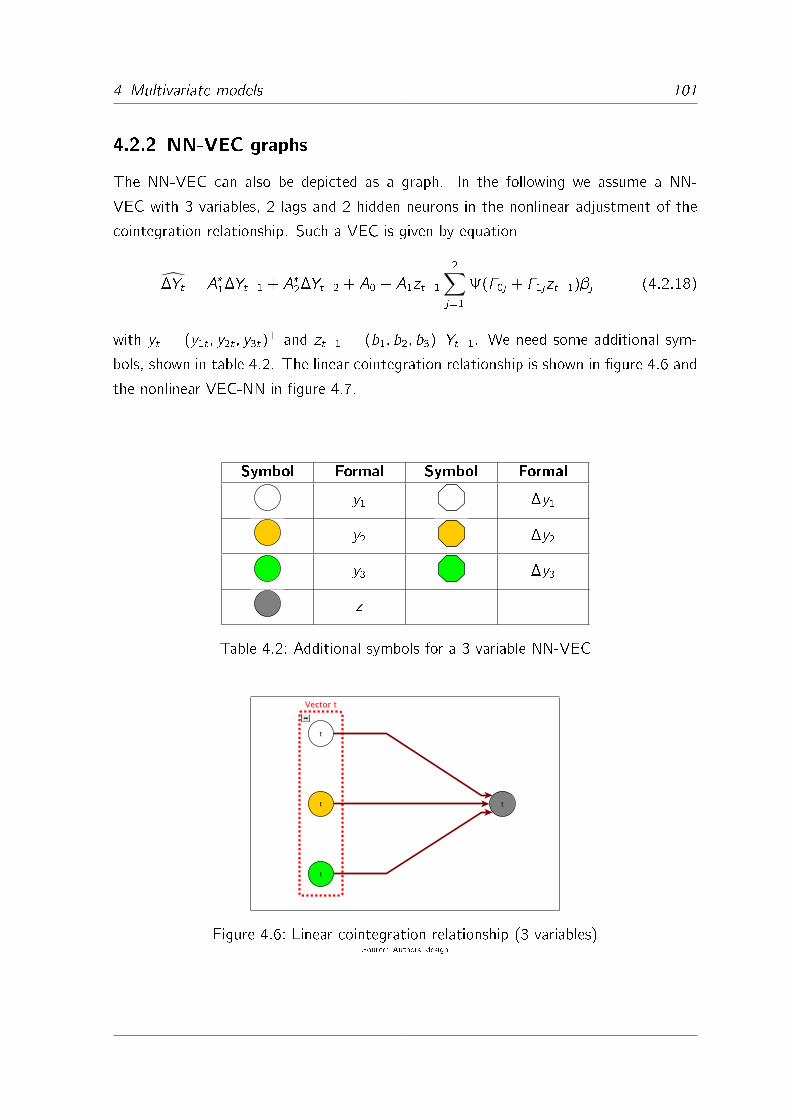
4 Multivariate models 101
4.2.2 NN-VEC graphs
The NN-VEC can also be depicted as a graph. In the following we assume a NN-
VEC with 3 variables, 2 lags and 2 hidden neurons in the nonlinear adjustment of the
cointegration relationship. Such a VEC is given by equation
�Yt = A�1�Yt�1 + A�2�Yt�2 + A0 + A1zt�1
2∑j=1
(�0j + �1jzt�1)�j (4.2.18)
with yt = (y1t ; y2t ; y3t)> and zt�1 = (b1; b2; b3)
>Yt�1. We need some additional sym-
bols, shown in table 4.2. The linear cointegration relationship is shown in �gure 4.6 and
the nonlinear VEC-NN in �gure 4.7.
Symbol Formal Symbol Formal
y1 �y1
y2 �y2
y3 �y3
z
Table 4.2: Additional symbols for a 3 variable NN-VEC
Figure 4.6: Linear cointegration relationship (3 variables)Source: Authors' design
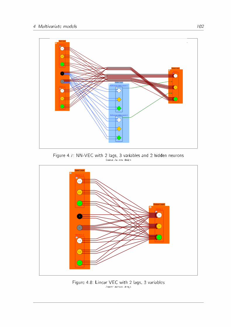
4 Multivariate models 102
Figure 4.7: NN-VEC with 2 lags, 3 variables and 2 hidden neuronsSource: Authors' design
Figure 4.8: Linear VEC with 2 lags, 3 variablesSource: Authors' design

4 Multivariate models 103
4.2.3 Identifying and Testing the NN-VEC
The nonlinear VEC of Escribano and Mira (2002) in combination with AR-NN from the
previous section (NN-VEC) is identi�ed via several steps. Partly we follow Dufrenot
and Mignon (2002) p.229 here. The steps are summarized in the following:
� Identify the linear cointegration relationship B>Yt�1. The easiest way is to use a
two or more stage least squares procedure (2SLS, 3SLS). Using the 2SLS proce-
dure to detect bivariate cointegration is for example discussed in Al-Ballaa (2005).
Therefore a structural equation system has to be constructed using the given vari-
ables. One or more variables included in the structural equation system a�ect the
cointegration relationship only indirectly via estimation of the instrumental vari-
able (they are not included in the cointegration relationship). A possible �eld
of application are supply-demand equations with nonlinear variables (supply and
demand observed over time are nonlinear). In the VEC-NN example from section
4.2.1.2 the result is an estimator for equation (4.2.14).
� Test the cointegration relationship on the �-mixing property. As there exist no
formal tests of �-mixing, tests on stationarity are su�cient.
� Estimate the NN-VEC using the Levenberg-Marquardt algorithm. Therefore the
m-dimensional NN-VEC has to be split into m equations which map on the uni-
variate R space (one equation for each variable). After this step the results in the
VEC-NN example from section 4.2.1.2 are the equations (4.2.15) and (4.2.16).
They can be brought together to receive the multivariate model (4.2.17).
� Test the nonlinear part of the nonlinear adjustment in the VEC on signi�cance.
It might be di�cult to compute the Wald statistic or the NIC for large m. A
simpler way, which in addition is focused on the out of sample behavior, is cross
validation (see section 3.4.1.2). Even a cointegration test can be executed using
cross validation: A linear VAR as well as NN-VEC with h = 0; : : : are estimated
(repeating step three for various h). If the out-of-sample performance of the VAR
is signi�cantly better than any NN-VEC, there is evidence for no cointegration.
Finally some remarks to the test on the mixing property in the cointegration relation-
ships: Tests on stationarity of the residuals are in general su�cient to guarantee the
�-mixing property. By de�nition �-mixing includes stationary processes. Dufrenot and

4 Multivariate models 104
Mignon (2002) use a response- surface (R/S) test in addition, but this does not con-
tribute any further �ndings. Therefore we will only consider stationarity in the empirical
part.

5 The German Automobile Industry and the US Market 105
5 The German Automobile Industry
and the US Market
The aim of this study is to predict some variables (macroeconomic, industry speci�c
and �nancial) connected with the German automobile industry using univariate AR-NNs
and a NN-VEC with one cointegration relationship. We use data from a time period
including the crisis of 2008/2009, which certainly is responsible for nonlinearities in the
data set. Mishkin (1996) p.17 de�nes a �nancial crisis as a nonlinear disruption to �nan-
cial markets.1 Such a de�nition restricted to �nancial markets can easily be transferred
to the real economy, in our case the German automobile industry. We observe that
data without crisis tend to be linear whereas data including a crisis tend to be nonlinear
(tables 5.2 and 5.4). Thus, especially for data including a crisis nonlinear methods are
necessary.
Our focus is particularly on the relations between the German automobile industry
and the US market. The macroeconomic variable is the exchange rate between US
Dollar and Euro (USD/EUR). We choose two industry speci�c variables: The �rst, the
industrial production of car manufacturers in Germany, can be considered as a supply
variable. The second, imports of foreign cars to the USA, serves as a demand variable.
As �nancial variable we use an index of the stock prices of three German car manu-
facturing companies. Several recent and past news (see for example Moody's (2008))
emphasise the special relationship between the German automobile manufacturers and
the US car market including the mentioned variables.
For the analysis of the data we �rst construct univariate AR-NN models for all vari-
ables, after we have shown that all series are nonlinear by the test of Lee, White and
Granger (1993) and integrated of order one by the RADF-test. We execute all the
variable selection procedures and parameter tests from chapter 3. The Levenberg-
Marquardt algorithm is used for parameter estimation. The resulting models are com-
1Although this paper is about asymmetric information, this statement of the de�nition a�ects �nancial
time series as well.
5 The German Automobile Industry and the US Market 106
pared to several linear AR and ARMA models. Afterwards a cointegrated model is
adjusted, whereas the cointegration relationship is calculated using a structural equa-
tion model and 2SLS regression. The cointegration relationship includes the variables
industry production of the German automobile industry, sales of foreign cars in the USA
and the exchange rate. The stock price index �ows indirectly into the cointegration
relationship, via estimation of the instrumental variable. We consider this �nancial
variable only as a management incentive, which indirectly exercises some in�uence on
industry production and sales. For calculations, some of the functions are implemented
in the statistical programming language R. The code is provided in appendix B. As far
as possible, some already existing R-packages as well as the software JMulti are used.
5.1 Economic Motivation
Before we proceed with the statistical analysis of the data, the economic motivation be-
hind the statistical models, especially a cointegrated model, should be explained. There-
fore at �rst the economic meaning of the technical terms in the NN-VEC is considered:
In the cointegrated model we distinguish between long-run and short-run e�ects. The
cointegration relationship, often referred to as long-run-equilibrium, represents the long
run e�ects, whereas the VAR part of the NN-VEC describes the short run e�ects.
Long- and short-run e�ects are combined by the NN-VEC. Intuitively we assume that
the univariate AR-NN are only able to describe short-run e�ects, as they do not include
any long-run economic relationship. This assumption is con�rmed by our results below.
A simple example should show how the long run relationship between industry pro-
duction, sales of foreign cars in the USA and the exchange rate are expected to explain
some economic developments: A long-run increase of the exchange rate, caused by a
weak USD, leads to lower sales of foreign cars in the USA and consequently a lower
industry production in the German car manufacturing industry. This statement is only
valid for the German premium car manufacturers (the diversi�ed VW corporation is not
much a�ected as its production for the US market is located in the NAFTA aerea and its
cars dont count as imported). In other words we consider the exchange rate exposure of
the German premium automobile industry with focus on sales and industry production.
Some statistics underline how important the US market for German car manufacturers
is (see VDA (2010)): In 2008 74.4% and in 2009 68.8% of the production of German
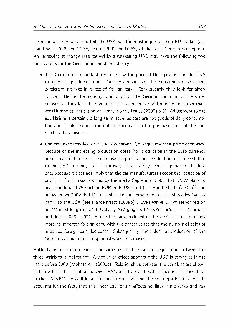
5 The German Automobile Industry and the US Market 107
car manufacturers was exported, the USA was the most important non-EU market (ac-
counting in 2008 for 12.6% and in 2009 for 10.5% of the total German car export).
An increasing exchange rate caused by a weakening USD may have the following two
implications on the German automobile industry:
� The German car manufacturers increase the price of their products in the USA
to keep the pro�t constant. On the demand side US consumers observe the
persistent increase in prices of foreign cars. Consequently they look for alter-
natives. Hence the industry production of the German car manufacturers de-
creases, as they lose their share of the important US automobile consumer mar-
ket (Humboldt Institution on Transatlantic Issues (2005) p.3). Adjustment to the
equilibrium is certainly a long-term issue, as cars are not goods of daily consump-
tion and it takes some time until the increase in the purchase price of the cars
reaches the consumer.
� Car manufacturers keep the prices constant. Consequently their pro�t decreases,
because of the increasing production costs (for production in the Euro currency
area) measured in USD. To increase the pro�t again, production has to be shifted
to the USD currency area. Intuitively, this strategy seems superior to the �rst
one, because it does not imply that the car manufacturers accept the reduction of
pro�t. In fact it was reported by the media September 2009 that BMW plans to
invest additional 750 million EUR in its US plant (see Handelsblatt (2009a)) and
in December 2009 that Daimler plans to shift production of the Mercedes C-class
partly to the USA (see Handelsblatt (2009b)). Even earlier BMW responded on
an assumed long-run weak USD by enlarging its US based production (Harbour
and Joas (2008) p.67). Hence the cars produced in the USA do not count any
more as imported foreign cars, with the consequence that the number of sales of
imported foreign cars decreases. Subsequently, the industrial production of the
German car manufacturing industry also decreases.
Both chains of reaction lead to the same result: The long-run-equilibrium between the
three variables is maintained. A vice versa e�ect appears if the USD is strong as in the
years before 2003 (Mohatarem (2003)). Relationships between the variables are shown
in �gure 5.1: The relation between EXC and IND and SAL respectively is negative.
In the NN-VEC the additional nonlinear term involving the cointegration relationship
accounts for the fact, that this linear equilibrium a�ects nonlinear time series and has
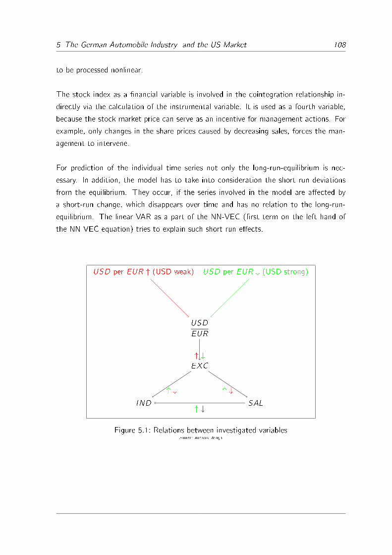
5 The German Automobile Industry and the US Market 108
to be processed nonlinear.
The stock index as a �nancial variable is involved in the cointegration relationship in-
directly via the calculation of the instrumental variable. It is used as a fourth variable,
because the stock market price can serve as an incentive for management actions. For
example, only changes in the share prices caused by decreasing sales, forces the man-
agement to intervene.
For prediction of the individual time series not only the long-run-equilibrium is nec-
essary. In addition, the model has to take into consideration the short run deviations
from the equilibrium. They occur, if the series involved in the model are a�ected by
a short-run change, which disappears over time and has no relation to the long-run-
equilibrium. The linear VAR as a part of the NN-VEC (�rst term on the left hand of
the NN-VEC equation) tries to explain such short-run-e�ects.
IND SAL
EXC
USD
EUR
USD per EUR " (USD weak) USD per EUR # (USD strong)
" #
" # " #
" #
Figure 5.1: Relations between investigated variablesSource: Authors' design

5 The German Automobile Industry and the US Market 109
5.2 The Data
We use monthly data from January 1999 to September 2009, therefore T = 129. The
�nancial data are provided by Thomson Banker One. Prices of the shares traded at
Frankfurt Stock Exchange are in Euro and are provided as monthly average closings.
Each company is represented by its most traded share, in detail Porsche Automobil Hold-
ing Vz, BMW St, and Daimler St. BMW and Daimler shares are common shares. The
Porsche share is a preferred share of Porsche Automobil Holding SE, which includes
100% of the Dr.Ing.h.c. F.Porsche AG. Common stocks of the Porsche Automobil
Holding SE are not traded on stock markets.
The German premium car manufacturer stock price index (PCI) is calculated as a
Laspeyres index by the following formula (see Moosmüller (2004) p.28)
PCIt =wp0 � pt + wb0 � bt + wd0 � dtwp0 � p0 + wb0 � b0 + wd0 � d0 : (5.2.1)
pt indicates the Porsche share, bt the BMW share, dt the Daimler share and w(�)0 the
weights belonging to the individual shares at time t = 0. As weights for a company we
use its sales (in Euro, also provided by Thomson Banker One) divided by the sum of
all companies sales in 1998. The weight factors are in detail wb0 = 0:19, wd0 = 0:79
and wp0 = 0:02. We use the logarithm of the series in the following. Figure 3.1 shows
the PCI time series in logarithms. Logarithms have to be used to bring this series in
accordance to the other ones concerning the behavior of the �rst di�erences. Although
the RADF test indicates that the original series is stationary in �rst di�erences, huge
outliers in the beginning of 2009 seem not to �t into the concept of a stationary series.
Logarithms smooth out those outliers.
The monthly Dollar to Euro (Dollar per 1 Euro) exchange rate (EXC) is provided
by the German Federal Reserve Bank (Bundesbank). It is plotted in �gure 3.3, �rst
di�erences in �gure 3.4. The industrial production of the German car manufacturing
and car parts manufacturing industry adjusted for working days (IND) is also provided
by the Bundesbank. As it is originally scaled di�erently than the other values, a simple
index is constructed with the average of 1999=100. The series is seasonally adjusted
using the R-package timsac. We assume an additive model and split o� the seasonal
components, such that the series only consists of the AR-part and the noise. The US

5 The German Automobile Industry and the US Market 110
Bureau of Economic Analysis provides the data on sales of foreign cars in the USA
(SAL). Originally the scale of the series is sold units in thousands. Hence to bring it in
accordance with the other data, an index with the average of 1999=100 is constructed.
The series is seasonal adjusted like the industry production series.
5 The German Automobile Industry and the US Market 111
Time
2000 2002 2004 2006 2008 2010
0.5
1.0
1.5
2.0
Time
2000 2002 2004 2006 2008 2010
-0.3
-0.2
-0.1
0.0
0.1
0.2
0.3
0.4
(Log-) PCI in levels (Log-) PCI in �rst di�erences
Time
2000 2002 2004 2006 2008 2010
1.0
1.2
1.4
1.6
Time
2000 2002 2004 2006 2008 2010
-0.10
-0.05
0.00
0.05
EXC in levels EXC in �rst di�erences
Time
2000 2002 2004 2006 2008 2010
0.9
1.0
1.1
1.2
1.3
1.4
1.5
Time
2000 2002 2004 2006 2008 2010
-0.10
-0.05
0.00
0.05
0.10
0.15
IND in levels IND in �rst di�erences
Time
2000 2002 2004 2006 2008 2010
1.0
1.2
1.4
1.6
Time
2000 2002 2004 2006 2008 2010
-0.4
-0.2
0.0
0.2
SAL in levels SAL in �rst di�erences
Figure 5.2: Data plotSource: Authors' design

5 The German Automobile Industry and the US Market 112
5.3 Nonlinearity and Stationarity Tests
Before AR-NN models can be adjusted the data have to be tested for stationarity. This
test requires a speci�cation of the lag-order, thus the test statistic is calculated for lag
orders from n = 1; : : : ; 4. We assume that a maximal lag order of m = 4 is su�cient,
with respect to keep the number of parameters in a realistic relation to the number of
observations T . In table 3.3 the RADF test statistic is calculated for levels and �rst
di�erences for all series for lag orders 1 to 4 without constant and trend variables in
the linear model (compare theorem 2.3). The function rank() in the basic package
was used to compute the ranks of the series, the function adfTest() in the R-package
fUnitRoots was used for calculation of the test statistics, critical values are taken
from table 2.3 for a series with 100 observations. We clearly see that all series are
nonstationary in levels and stationary in �rst di�erences (in other words integrated of
order one).
But before AR-NN models are adjusted at the �rst di�erences of the series, their non-
linearity has to be examined. Therefore the Teräsvirta-Lin-Granger test (see section
3.1.2.2) with polynomial (3.1.20) is used. The R-package tseries provides a function
terasvirta.test(), which is used to calculate the results. They are shown in tables
5.2 and 5.3. Note that here T=128 because of the di�erentiation. It is observable that
all series are nonlinear at least for lag orders >1.
As already mentioned above the data contain the crisis of 2008/2009. We now want to
examine, if the crisis is responsible for the nonlinearity. Thus we test parts of the series
without crisis (the �rst 100 values representing the time period from January 1999 to
April 2007) for nonlinearity. The �2- test statistic for the Lee-Teräsvirta-Granger test
is shown in table 5.4. In fact it is observable, that series without crisis data tend to
be linear. This result compared to the result above (table 5.2) outlines the nonlinear
character of crises.
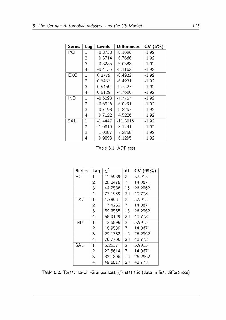
5 The German Automobile Industry and the US Market 113
Series Lag Levels Di�erences CV (5%)
PCI 1 -0.3733 -8.1096 -1.92
2 -0.3714 -6.7666 -1.92
3 -0.3285 -5.0388 -1.92
4 -0.4135 -5.1162 -1.92
EXC 1 0.2779 -8.4932 -1.92
2 0.5457 -6.4931 -1.92
3 0.5455 -5.7527 -1.92
4 0.6129 -4.7600 -1.92
IND 1 -0.6298 -7.7757 -1.92
2 -0.6926 -6.0291 -1.92
3 -0.7198 -5.2267 -1.92
4 -0.7122 -4.5226 -1.92
SAL 1 -1.4447 -11.3016 -1.92
2 -1.0810 -8.1241 -1.92
3 -1.0387 -7.2868 -1.92
4 -0.9093 -6.1205 -1.92
Table 5.1: ADF test
Series Lag �2 df CV (95%)
PCI 1 11.5989 2 5.9915
2 20.2478 7 14.0671
3 44.2536 16 26.2962
4 77.1989 30 43.773
EXC 1 4.7863 2 5.9915
2 17.4252 7 14.0671
3 39.6585 16 26.2962
4 58.0129 20 43.773
IND 1 12.5899 2 5.9915
2 18.9509 7 14.0671
3 29.1732 16 26.2962
4 76.7795 20 43.773
SAL 1 6.2537 2 5.9915
2 22.5614 7 14.0671
3 33.1896 16 26.2962
4 49.5517 20 43.773
Table 5.2: Teräsvirta-Lin-Granger test �2- statistic (data in �rst di�erences)
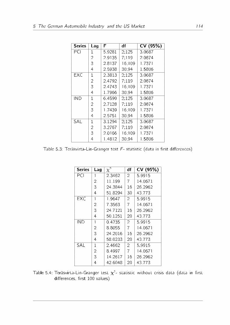
5 The German Automobile Industry and the US Market 114
Series Lag F df CV (95%)
PCI 1 5.9281 2;125 3.0687
2 2.9135 7;119 2.0874
3 2.8137 16;109 1.7371
4 2.5938 30;94 1.5806
EXC 1 2.3813 2;125 3.0687
2 2.4792 7;119 2.0874
3 2.4743 16;109 1.7371
4 1.7966 30;94 1.5806
IND 1 6.4599 2;125 3.0687
2 2.7128 7;119 2.0874
3 1.7439 16;109 1.7371
4 2.5751 30;94 1.5806
SAL 1 3.1294 2;125 3.0687
2 3.2767 7;119 2.0874
3 2.0166 16;109 1.7371
4 1.4812 30;94 1.5806
Table 5.3: Teräsvirta-Lin-Granger test F - statistic (data in �rst di�erences)
Series Lag �2 df CV (95%)
PCI 1 2.3462 2 5.9915
2 11.199 7 14.0671
3 24.3844 16 26.2962
4 51.8294 30 43.773
EXC 1 1.9647 2 5.9915
2 7.3563 7 14.0671
3 24.7121 16 26.2962
4 50.1251 20 43.773
IND 1 0.4235 2 5.9915
2 8.8055 7 14.0671
3 24.2016 16 26.2962
4 58.0233 20 43.773
SAL 1 2.4662 2 5.9915
2 8.4997 7 14.0671
3 14.2617 16 26.2962
4 42.6048 20 43.773
Table 5.4: Teräsvirta-Lin-Granger test �2- statistic without crisis data (data in �rst
di�erences, �rst 100 values)

5 The German Automobile Industry and the US Market 115
5.4 Univariate AR-NN
5.4.1 Lag Selection
We use the series in �rst di�erences as a starting point for lag selection, because the
lag selection procedures in section 3.2 are only appropriate for stationary series. Figure
5.3 shows the AC and PAC for all series up to lag order 10. In the �gure the interval
[� 2pT; 2p
T]=[�0:177; 0:177] is marked by a dashed line. The PAC is above that dashed
line for the IND series at lag 1 and for the SAL series at lag 2. This information can
be used for lag selection, but we still have no indication for the lag order for the �rst
two series.
Hence we subsequently apply the other lag selection procedures proposed in section
3.2. The MIC is - like the AC - not a very useful tool for lag selection. The MIC,
calculated by the function in appendix B.3 with d = 100, for the �rst 4 lags are shown
in table 5.5. It is observable that the results are in the same range as the jACj. Resultsfor polynomial lag selection using formula (3.2.17) and the AIC and the BIC as quality
criteria are displayed in table 5.6. For the calculations the function in appendix B.2 is
used, the optimal lag orders are marked by a "*". AIC and BIC accord in only one
case. The AIC sometimes also tends to include more lags than the BIC. The next table
(table 5.7) shows results for the Nonlinear Final Prediction Error (NFPE) from section
3.2.4. For calculation of the results the software JMulti was used. The AFPE as well
as its correction, the CAFPE , are calculated. Both criteria have to be minimized like
any other IC. It is observable that both criterions indicate the same optimal lag order.
As the di�erent lag selection procedures lead to partly very di�erent results, we have
to decide which lag order we use in the following. We proceed with the results from
polynomial lag selection and use the AIC, thus the PCI has 4 lags, the EXC series has
3 lags and the IND and the SAL series have 2 lags.

5 The German Automobile Industry and the US Market 116
Lags
Series 1 2 3 4
PCI 0.0164 0.0312 0.0448 0.0575
EXC 0.0675 0.0979 0.1208 0.1399
IND 0.0243 0.0448 0.0627 0.0788
SAL 0.0116 0.0225 0.0328 0.0426
Table 5.5: MIC
Series Lag AIC BIC
PCI 1 -215.2964 �218:0006�2 -213.1339 -213.4044
3 -209.6199 -203.8683
4 �216:0644� -195.3435
EXC 1 -538.8916 �541:5958�2 -535.8858 -536.1562
3 �541:6615� -535.9100
4 -538.0680 -517.3471
IND 1 -428.1411 -430.8452
2 �435:8922� �436:1626�3 -428.1819 -422.4304
4 -430.2283 -409.5074
SAL 1 -210.4986 -213.2028
2 �224:1334� �224:4039�3 -220.1187 -214.3672
4 -214.0852 -193.3643
Table 5.6: Polynomial approximation lag selection

5 The German Automobile Industry and the US Market 117
02
46
810
-0.2 0.0 0.2 0.4 0.6 0.8 1.0
Lag
ACF
24
68
10
-0.15 -0.05 0.00 0.05 0.10 0.15
Lag
Partial ACF
AC PCI PAC PCI
02
46
810
-0.2 0.0 0.2 0.4 0.6 0.8 1.0
Lag
ACF
24
68
10
-0.1 0.0 0.1 0.2 0.3
Lag
Partial ACF
AC EXC PAC EXC
02
46
810
-0.2 0.0 0.2 0.4 0.6 0.8 1.0
Lag
ACF
24
68
10
-0.1 0.0 0.1 0.2
Lag
Partial ACF
AC IND PAC IND
02
46
810
-0.2 0.0 0.2 0.4 0.6 0.8 1.0
Lag
ACF
24
68
10
-0.2 -0.1 0.0 0.1
Lag
Partial ACF
AC SAL PAC SAL
Figure 5.3: AC and PACSource: Authors' design
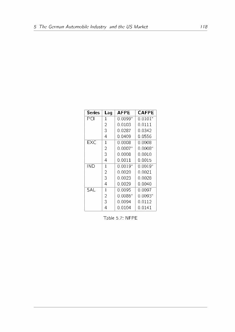
5 The German Automobile Industry and the US Market 118
Series Lag AFPE CAFPE
PCI 1 0:0099� 0:0101�
2 0.0103 0.0111
3 0.0287 0.0342
4 0.0409 0.0556
EXC 1 0.0008 0.0008
2 0:0007� 0:0008�
3 0.0008 0.0010
4 0.0011 0.0015
IND 1 0:0019� 0:0019�
2 0.0020 0.0021
3 0.0023 0.0028
4 0.0029 0.0040
SAL 1 0.0095 0.0097
2 0:0086� 0:0093�
3 0.0094 0.0112
4 0.0104 0.0141
Table 5.7: NFPE
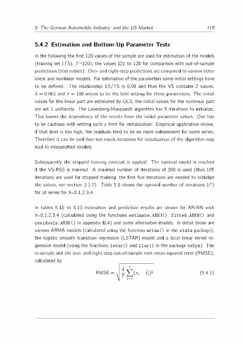
5 The German Automobile Industry and the US Market 119
5.4.2 Estimation and Bottom-Up Parameter Tests
In the following the �rst 120 values of the sample are used for estimation of the models
(training set (TS), T=120), the values 121 to 128 for comparison with out-of-sample
predictions (test subset). One- and eight-step predictions are compared to various other
linear and nonlinear models. For estimation of the parameters some initial settings have
to be de�ned. The relationship ES/TS is 0.98 and thus the VS contains 2 values.
� = 0:001 and � = 100 seems to be the best setting for those parameters. The initial
values for the linear part are estimated by OLS, the initial values for the nonlinear part
are set 1 uniformly. The Levenberg-Marquardt algorithm has 5 iterations to initialize.
This lowers the dependency of the results from the initial parameter values. One has
to be cautious with setting such a limit for initialization: Empirical application shows,
if that limit is too high, the residuals tend to be no more independent for some series.
Therefore it can be said that too much iterations for initialization of the algorithm may
lead to misspeci�ed models.
Subsequently the stopped training concept is applied: The optimal model is reached
if the VS-RSS is minimal. A maximal number of iterations of 200 is used (thus 195
iterations are used for stopped training, the �rst �ve iterations are needed to initialize
the values, see section 3.3.7). Table 5.8 shows the optimal number of iterations (i*)
for all series for h=0,1,2,3,4.
In tables 5.10 to 5.13 estimation and prediction results are shown for AR-NN with
h=0,1,2,3,4 (calculated using the functions estimate.ARNN(), fitted.ARNN() and
residuals.ARNN() in appendix B.4) and some alternative models. In detail those are
various ARMA models (calculated using the function arima() in the stats package),
the logistic smooth transition regression (LSTAR) model and a local linear kernel re-
gression model (using the functions lstar() and llar() in the package tsDyn). The
in-sample and the one- and eight step out-of-sample root mean-squared error (RMSE),
calculated by
RMSE =
√√√√ 1
T
T∑t=1
(xt � xt)2 (5.4.1)

5 The German Automobile Industry and the US Market 120
for in-sample and
RMSE =
√√√√1
k
k∑t=T+1
(xt � xt)2 (5.4.2)
for the k-step prediction are shown in the tables as performance measure. The in-sample
RMSE of the models trained by cross-validation stopping can not be compared to the
RMSE of the alternative models. They only minimize the RSS of the TS, whereas
the cross-validation stopping method also considers the prediction behavior during the
estimation process (VS as part of the TS). A fairer comparison is the application of
the ES-RMSE as in-sample measure for the AR-NN's. It is minimized analogously to
the in-sample RMSE in the alternative models. Note that di�erent variances for the
individual steps in more-step prediction might distort the RMSE. A rolling one-step
prediction would overcome that problem. However more-step prediction is a realistic
aim in forecasting time series, thus we apply it despite that. The �gure 5.4 should be
considered in together with the RMSE for more-step prediction. In addition tables 5.10
to 5.13 show the Theil inequality coe�cient (IEC) for the out-of-sample set. The Theil
IEC for a k-step prediction is calculated by
Theil IEC =
√√√√ ∑k
t=T+1(xt � xt)2∑k
t=T+1(xt � 1T
∑T
t=1 xt)2: (5.4.3)
It compares the out-of-sample prediction with the mean of the TS. If the Theil IEC is
small, the out-of-sample prediction is better, if it is larger than one, the mean of the TS
(average of the TS) is better (see Steurer (1996) p.120). The Theil IEC also simpli�es
the comparison of the out-of-sample performance of the models between each other,
because it normalizes the RMSE (by the division of the out-of-sample MSE by the mean
of the TS MSE).
To identify the optimal model we use the two bottom-up procedures proposed in section
3.4.1:
� Table 5.9 shows the Lee-White-Granger bottom up test for h=1 using the models
estimated in tables 5.10 to 5.13 (calculated using the function LWG.test() in
appendix B.9). We only use the �rst 118 values to calculate the test statistic.
This is necessary because the Lee-White-Granger test is based on the in-sample
performance for RSS minimizing procedures. If models are estimated using the

5 The German Automobile Industry and the US Market 121
stopped training method, only the ES is considered to be in-sample and is mini-
mized like in least squares procedures. Including the VS would distort the results
of the test. We execute the test for the model with h=1 (the test for h=0 equals
the linearity test which was already executed in section 5.3). The test indicates,
that for none of the series a second hidden neuron would improve the model.
The statement of the test is correct if the third column in tables 5.10 to 5.13
are considered. If the focus is mainly on in-sample behavior of the models, the
estimation procedure could be stopped after the models with h=1 are estimated.
� As we are also interested in the out-of-sample performance, cross validation con-
sidering the one- or eight- step- prediction would be an alternative. We assume
that the models with the lowest out-of-sample RMSE are optimal. Concerning
the one step prediction those are the AR-NN with h=4 for PCI and EXC, h=1
for IND and h=0 for SAL. If the eight-step prediction is considered the optimal
models have h=4 for PCI, EXC and IND and again h=0 for SAL. Consequently
the SAL series is linear (in contrast to the result of the nonlinearity test).
We proceed with the analysis of the models which perform best concerning the one-step
prediction. In �gure 5.4 the in-sample behavior is plotted, �gure 5.5 shows the out-of-
sample performance compared to a linear AR and a ARMA model. As the AR-NN for
SAL has h=0, it does not di�er from the linear AR model. In particular in the short-
run prediction (1-3 steps) the AR-NN performs better than linear models, whereas for
higher steps of prediction they become similar to the linear AR.
Tables 5.14 to 5.17 show the parameters for the mentioned models. Interpretation
of the parameters is certainly more di�cult than in linear models - if not impossible.
One argument might be that the larger the parameter for a variable in one hidden neu-
ron is, the more this variable contributes to the nonlinearity of the hidden neuron. Note
that for the models with h=4 the parameters in all hidden neurons are the same. If only
one hidden neuron with �= 4 � �j would be used instead, the results would be identical.
This could be one way to reduce the complexity.2
2This result depends from the initial settings. For di�erent settings, the parameters in each hidden
neuron di�er from each other.
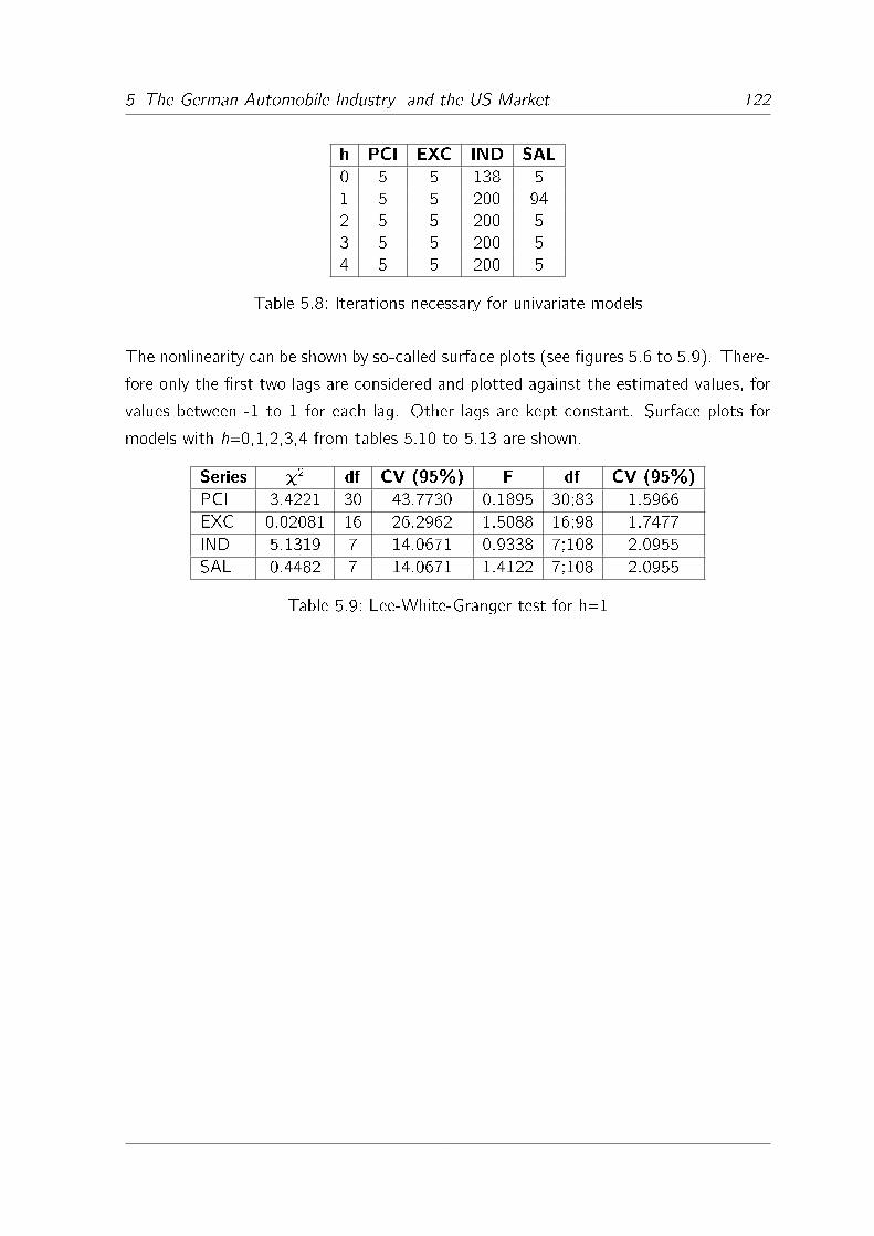
5 The German Automobile Industry and the US Market 122
h PCI EXC IND SAL
0 5 5 138 5
1 5 5 200 94
2 5 5 200 5
3 5 5 200 5
4 5 5 200 5
Table 5.8: Iterations necessary for univariate models
The nonlinearity can be shown by so-called surface plots (see �gures 5.6 to 5.9). There-
fore only the �rst two lags are considered and plotted against the estimated values, for
values between -1 to 1 for each lag. Other lags are kept constant. Surface plots for
models with h=0,1,2,3,4 from tables 5.10 to 5.13 are shown.
Series �2 df CV (95%) F df CV (95%)
PCI 3.4221 30 43.7730 0.1895 30;83 1.5966
EXC 0.02081 16 26.2962 1.5088 16;98 1.7477
IND 5.1319 7 14.0671 0.9338 7;108 2.0955
SAL 0.4482 7 14.0671 1.4122 7;108 2.0955
Table 5.9: Lee-White-Granger test for h=1

5 The German Automobile Industry and the US Market 123
In-
sample
Out-of-sample
1
stepprediction
Out-of-sample
8
stepprediction
Model
rRMSE
RMSE
TheilIEC
RMSE
TheilIEC
AR-N
N's
AR-NN(4),h=0
50.0900
0.3084
1.005
0.1957
0.9991
AR-NN(4),h=1
11
0.0898
0.3013
0.9819
0.1954
0.9974
AR-NN(4),h=2
17
0.0897
0.2698
0.8791
0.1905
0.9722
AR-NN(4),h=3
23
0.0898
0.2634
0.8583
0.1892
0.9658
AR-NN(4),h=4
29
0.0900
0.2624
0.8553
0.1889
0.9640
Alternatives
AR(4)
50.0915
0.3191
1.0397
0.1969
1.0051
ARMA(4,1)
60.0915
0.3180
1.0363
0.1985
1.0132
ARMA(4,5)
10
0.0844
0.3258
1.0617
0.2221
1.1337
LSTAR(4)
10
0.0869
0.3401
1.1083
0.2043
1.0429
LLAR(4)
-0.0964
0.3242
1.0565
0.1975
1.0081
Table5.10:PCI:AR-NNvs.other
models

5 The German Automobile Industry and the US Market 124
In-
sample
Out-of-sample
1
stepprediction
Out-of-sample
8
stepprediction
Model
rRMSE
RMSE
TheilIEC
RMSE
TheilIEC
AR-N
N's
AR-NN(3),h=0
40.0276
0.0284
0.6871
0.0287
0.9674
AR-NN(3),h=1
90.0270
0.0314
0.7597
0.0272
0.9169
AR-NN(3),h=2
14
0.0271
0.0272
0.6581
0.0266
0.8966
AR-NN(3),h=3
19
0.0271
0.0236
0.5710
0.0262
0.8831
AR-NN(3),h=4
24
0.0272
0.0208
0.5032
0.0260
0.8764
Alternatives
AR(3)
40.0288
0.0258
0.6242
0.0277
0.9337
ARMA(3,1)
50.0288
0.0264
0.6387
0.0277
0.9337
ARMA(3,5)
90.0272
0.0375
0.9073
0.0292
0.9843
LSTAR(3)
90.0263
0.0817
1.9766
0.0255
0.8596
LLAR(3)
-0.0303
0.0829
2.0056
0.0270
0.9101
Table5.11:EXC:AR-NNvs.other
models

5 The German Automobile Industry and the US Market 125
In-
sample
Out-of-sample
1
stepprediction
Out-of-sample
8
stepprediction
Model
rRMSE
RMSE
TheilIEC
RMSE
TheilIEC
AR-N
N's
AR-NN(2),h=0
30.0388
0.1274
1.3913
0.0765
1.1075
AR-NN(2),h=1
70.0378
0.0122
0.1332
0.0690
0.9990
AR-NN(2),h=2
11
0.0378
0.0241
0.2632
0.0652
0.9439
AR-NN(2),h=3
15
0.0378
0.0316
0.3451
0.0642
0.9295
AR-NN(2),h=4
19
0.0378
0.0374
0.4084
0.0639
0.9251
Alternatives
AR(2)
30.0415
0.0916
1.0004
0.0715
1.0352
ARMA(2,1)
40.0410
0.0616
0.6727
0.0903
1.3073
ARMA(2,5)
80.0399
0.0509
0.5559
0.0973
1.4087
LSTAR(2)
80.0378
0.2664
2.9094
0.1424
2.0616
LLAR(2)
-0.0445
0.1358
1.4831
0.0748
1.0829
Table5.12:IND:AR-NNvs.other
models

5 The German Automobile Industry and the US Market 126
In-
sample
Out-of-sample
1
stepprediction
Out-of-sample
8
stepprediction
Model
rRMSE
RMSE
TheilIEC
RMSE
TheilIEC
AR-N
N's
AR-NN(2),h=0
30.0905
0.0104
0.3664
0.2311
0.999
AR-NN(2),h=1
70.0879
0.0223
0.7855
0.2316
1.0012
AR-NN(2),h=2
11
0.0881
0.0178
0.627
0.2312
0.9994
AR-NN(2),h=3
15
0.0883
0.0168
0.5918
0.2312
0.9994
AR-NN(2),h=4
19
0.0884
0.0164
0.5777
0.2312
0.9994
Alternatives
AR(2)
30.0903
0.0107
0.3769
0.2311
0.999
ARMA(2,1)
40.0896
0.007
0.2466
0.2315
1.0007
ARMA(2,5)
80.0860
0.1019
3.5896
0.2360
1.0202
LSTAR(2)a
--
--
--
LLAR(2)
-0.0942
0.0107
0.3769
0.2311
0.999
Table5.13:SAL:AR-NNvs.other
models
aNote
thattheLSTARmodelwasnotcalculated,because
theRfunctionindicated,thattheseries
islinear

5 The German Automobile Industry and the US Market 127
0 20 40 60 80 100 120
-0.3
-0.2
-0.1
0.0
0.1
0.2
Time
OriginalES+ / − σ
PCI: In-sample AR-NN(4) with h=4
0 20 40 60 80 100 120
-0.10
-0.05
0.00
0.05
Time
OriginalES+ / − σ
EXC: In-sample AR-NN(3) with h=4
0 20 40 60 80 100 120
-0.10
-0.05
0.00
0.05
0.10
Time
OriginalES+ / − σ
IND: In-sample AR-NN(2) with h=1
0 20 40 60 80 100 120
-0.2
-0.1
0.0
0.1
0.2
Time
OriginalES+ / − σ
SAL: In-sample AR-NN(2) with h=0
Figure 5.4: Univariate models in-sample plotsSource: Authors' design
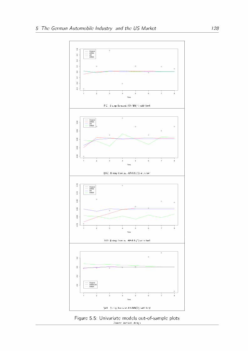
5 The German Automobile Industry and the US Market 128
1 2 3 4 5 6 7 8
-0.3
-0.2
-0.1
0.0
0.1
0.2
0.3
0.4
Time
OriginalARNNARARMA
PCI: 8 step forecast AR-NN(4) with h=4
1 2 3 4 5 6 7 8
-0.04
-0.02
0.00
0.02
0.04
Time
OriginalARNNARARMA
EXC: 8 step forecast AR-NN(3) with h=4
1 2 3 4 5 6 7 8
-0.10
-0.05
0.00
0.05
0.10
0.15
Time
OriginalARNNARARMA
IND: 8 step forecast AR-NN(2) with h=1
1 2 3 4 5 6 7 8
-0.4
-0.2
0.0
0.2
Time
OriginalARNN,ARARMA
SAL: 8 step forecast AR-NN(2) with h=0
Figure 5.5: Univariate models out-of-sample plotsSource: Authors' design

5 The German Automobile Industry and the US Market 129
�0= -0.3247 01= 0.6347 02= 0.6347
�1= -0.2901 11= 1.0051 12= 1.0051
�2= -0.2620 21= 0.7245 22= 0.7245
�3= -0.5168 31= 1.1304 32= 1.1304
�4=-0.3209 41= 0.6106 42= 0.6106
�1= 0.1499 �2= 0.1499
03= 0.6347 04= 0.6347
13= 1.0051 14= 1.0051
23= 0.7245 24= 0.7245
33= 1.1304 34= 1.1304
34= 0.6106 44= 0.6106
�3= 0.1499 �4= 0.1499
Table 5.14: PCI: Parameters AR-NN(4) with h=4
�0=-0.8535 01=1.0348 02= 1.0348
�1=-0.1592 11= 1.2125 12= 1.2125
�2=-0.6814 21= 1.2985 22= 1.2985
�3=-0.2733 31= 0.8475 32= 0.8475
�1= 0.2757 �2= 0.2757
03= 1.0348 04= 1.0348
13= 1.2125 14= 1.2125
23= 1.2985 24= 1.2985
33= 0.8475 34= 0.8475
�3= 0.2757 �4= 0.2757
Table 5.15: EXC: Parameters AR-NN(3) with h=4

5 The German Automobile Industry and the US Market 130
�0=-1.1246 01= 1.0516
�1=-1.4247 11= 1.9216
�2=-1.6643 21= 2.9492
�1= 1.4468
Table 5.16: IND: Parameters AR-NN(2) with h=1
�0= 0.0008
�1= -0.2710
�2= -0.1212
Table 5.17: SAL: Parameters AR-NN(2) with h=0
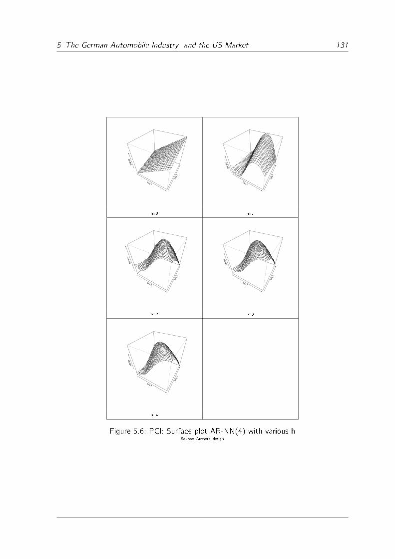
5 The German Automobile Industry and the US Market 131
Lag 1
Lag
2
AR-NN
Lag 1
Lag
2
AR-NN
h=0 h=1
Lag 1
Lag
2
AR-NN
Lag 1
Lag
2
AR-NN
h=2 h=3
Lag 1
Lag
2
AR-NN
h=4
Figure 5.6: PCI: Surface plot AR-NN(4) with various hSource: Authors' design
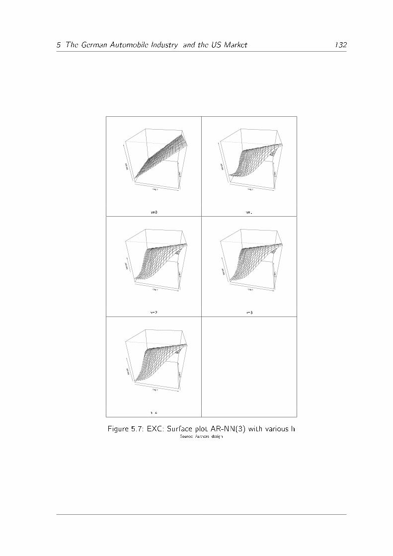
5 The German Automobile Industry and the US Market 132
Lag 1
Lag 2
AR-NN
Lag 1
Lag 2
AR-NN
h=0 h=1
Lag 1
Lag 2
AR-NN
Lag 1
Lag 2
AR-NN
h=2 h=3
Lag 1
Lag 2
AR-NN
h=4
Figure 5.7: EXC: Surface plot AR-NN(3) with various hSource: Authors' design
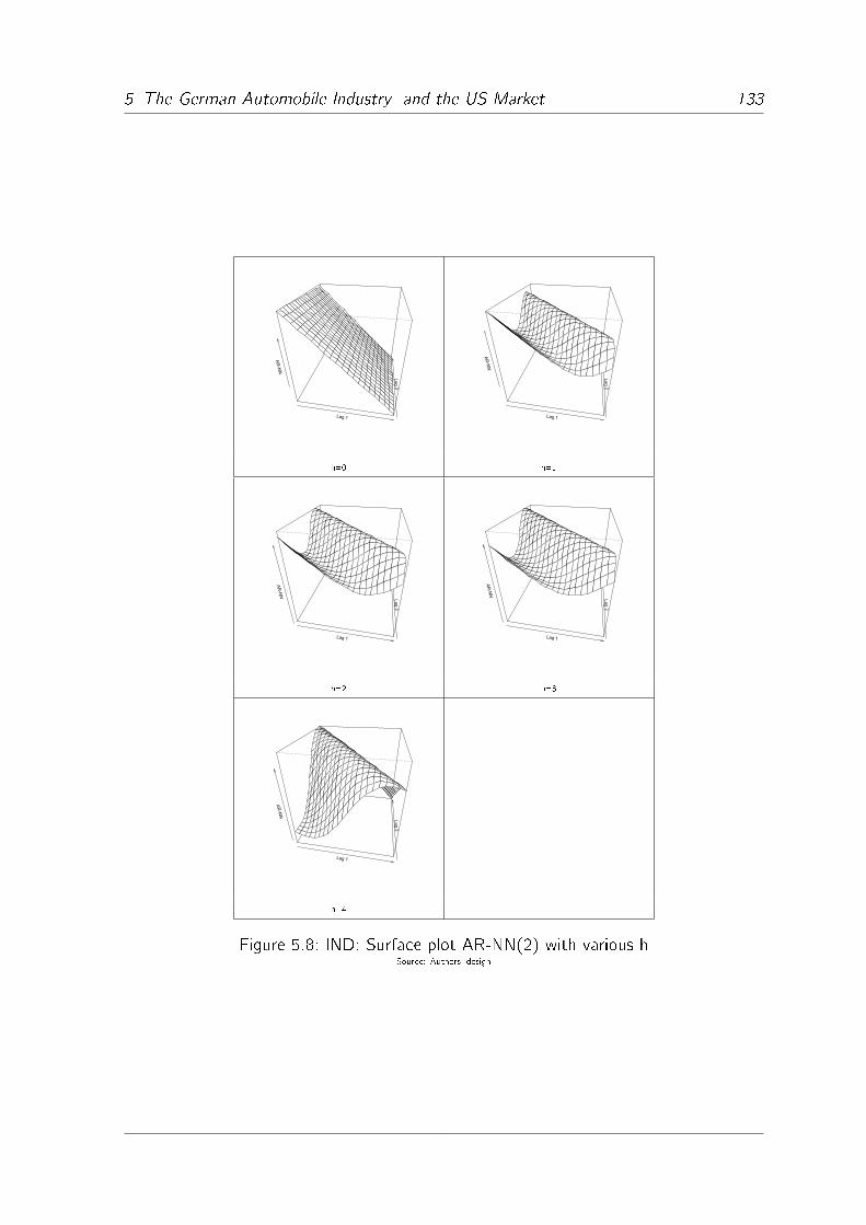
5 The German Automobile Industry and the US Market 133
Lag 1
Lag 2
AR-NN
Lag 1
Lag 2
AR-NN
h=0 h=1
Lag 1
Lag 2
AR-NN
Lag 1
Lag 2
AR-NN
h=2 h=3
Lag 1
Lag 2
AR-NN
h=4
Figure 5.8: IND: Surface plot AR-NN(2) with various hSource: Authors' design
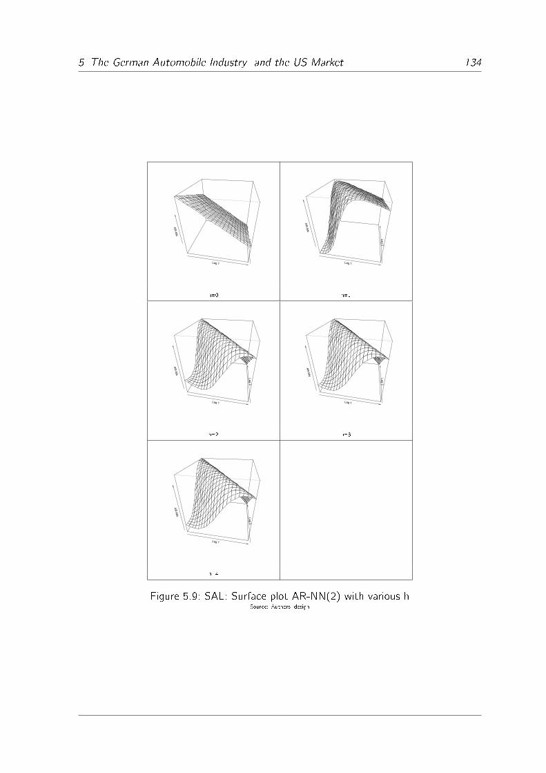
5 The German Automobile Industry and the US Market 134
Lag 1
Lag 2
AR-NN
Lag 1
Lag 2
AR-NN
h=0 h=1
Lag 1
Lag 2
AR-NN
Lag 1
Lag 2
AR-NN
h=2 h=3
Lag 1
Lag 2
AR-NN
h=4
Figure 5.9: SAL: Surface plot AR-NN(2) with various hSource: Authors' design
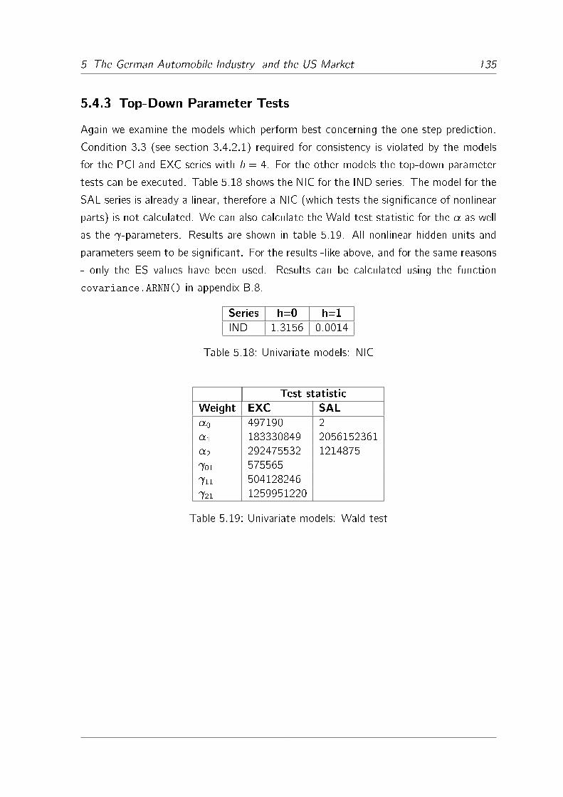
5 The German Automobile Industry and the US Market 135
5.4.3 Top-Down Parameter Tests
Again we examine the models which perform best concerning the one step prediction.
Condition 3.3 (see section 3.4.2.1) required for consistency is violated by the models
for the PCI and EXC series with h = 4. For the other models the top-down parameter
tests can be executed. Table 5.18 shows the NIC for the IND series. The model for the
SAL series is already a linear, therefore a NIC (which tests the signi�cance of nonlinear
parts) is not calculated. We can also calculate the Wald test statistic for the � as well
as the -parameters. Results are shown in table 5.19. All nonlinear hidden units and
parameters seem to be signi�cant. For the results -like above, and for the same reasons
- only the ES values have been used. Results can be calculated using the function
covariance.ARNN() in appendix B.8.
Series h=0 h=1
IND 1.3156 0.0014
Table 5.18: Univariate models: NIC
Test statistic
Weight EXC SAL
�0 497190 2
�1 183330849 2056152361
�2 292475532 1214875
01 575565
11 504128246
21 1259951220
Table 5.19: Univariate models: Wald test
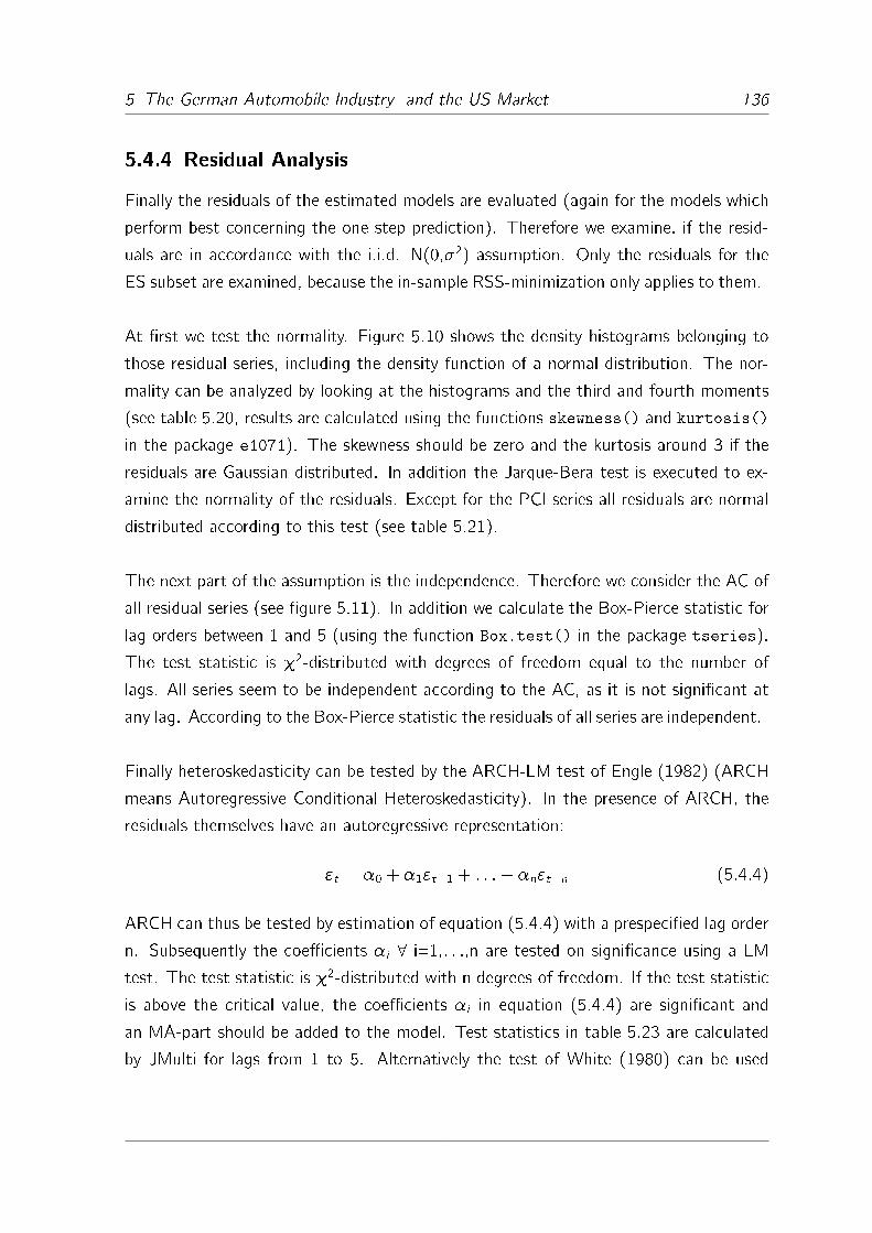
5 The German Automobile Industry and the US Market 136
5.4.4 Residual Analysis
Finally the residuals of the estimated models are evaluated (again for the models which
perform best concerning the one step prediction). Therefore we examine, if the resid-
uals are in accordance with the i.i.d. N(0,�2) assumption. Only the residuals for the
ES subset are examined, because the in-sample RSS-minimization only applies to them.
At �rst we test the normality. Figure 5.10 shows the density histograms belonging to
those residual series, including the density function of a normal distribution. The nor-
mality can be analyzed by looking at the histograms and the third and fourth moments
(see table 5.20, results are calculated using the functions skewness() and kurtosis()
in the package e1071). The skewness should be zero and the kurtosis around 3 if the
residuals are Gaussian distributed. In addition the Jarque-Bera test is executed to ex-
amine the normality of the residuals. Except for the PCI series all residuals are normal
distributed according to this test (see table 5.21).
The next part of the assumption is the independence. Therefore we consider the AC of
all residual series (see �gure 5.11). In addition we calculate the Box-Pierce statistic for
lag orders between 1 and 5 (using the function Box.test() in the package tseries).
The test statistic is �2-distributed with degrees of freedom equal to the number of
lags. All series seem to be independent according to the AC, as it is not signi�cant at
any lag. According to the Box-Pierce statistic the residuals of all series are independent.
Finally heteroskedasticity can be tested by the ARCH-LM test of Engle (1982) (ARCH
means Autoregressive Conditional Heteroskedasticity). In the presence of ARCH, the
residuals themselves have an autoregressive representation:
"t = �0 + �1"t�1 + : : :+ �n"t�n (5.4.4)
ARCH can thus be tested by estimation of equation (5.4.4) with a prespeci�ed lag order
n. Subsequently the coe�cients �i 8 i=1,: : :,n are tested on signi�cance using a LM
test. The test statistic is �2-distributed with n degrees of freedom. If the test statistic
is above the critical value, the coe�cients �i in equation (5.4.4) are signi�cant and
an MA-part should be added to the model. Test statistics in table 5.23 are calculated
by JMulti for lags from 1 to 5. Alternatively the test of White (1980) can be used

5 The German Automobile Industry and the US Market 137
to examine the residuals on heteroskedasticity. We �nd heteroskedasticity only in the
residuals of SAL.
Series Mean � Skewness Kurtosis
PCI 0.0000 0.0903 0.4794 1.15
EXC 0.0000 0.0274 -0.0511 1.3464
IND 0.0000 0.0379 -0.1335 0.0380
SAL 0.0000 0.0909 -0.0578 -0.0518
Table 5.20: Univariate models: Skewness and kurtosis
Series Test statistic CV (99%)
PCI 11.9703 9.2103
EXC 9.981 9.2103
IND 0.3996 9.2103
SAL 0.0674 9.2103
Table 5.21: Univariate models: Jarque-Bera test
Lag
Series 1 2 3 4 5
PCI 0.0128 0.0132 0.0419 0.0804 0.3013
EXC 0.0409 0.5757 2.2220 2.4138 2.4189
IND 0.0000 0.0263 0.3475 0.3476 0.4387
SAL 0.0062 0.0076 0.0366 3.4300 3.4877
CV (95%) 3.8415 5.9915 7.8147 9.4877 11.071
CV (99%) 6.6349 9.2103 11.3449 13.2767 15.0863
Table 5.22: Univariate models: Box-Pierce test
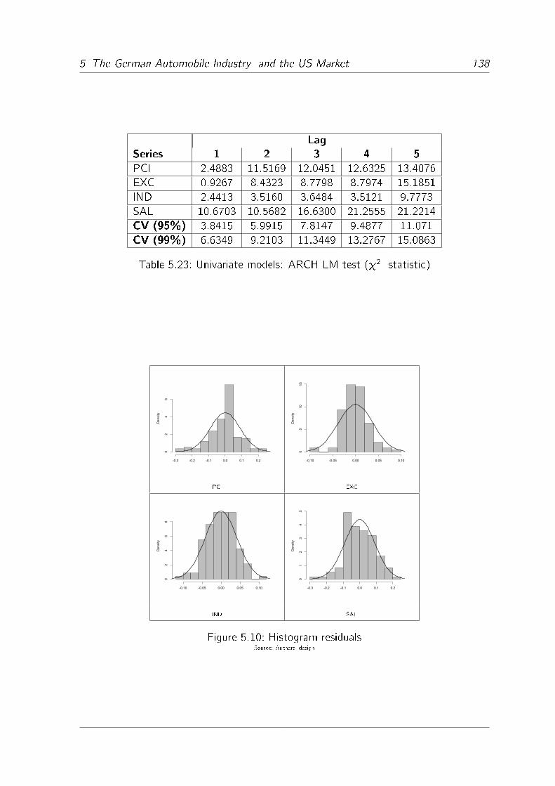
5 The German Automobile Industry and the US Market 138
Lag
Series 1 2 3 4 5
PCI 2.4883 11.5169 12.0451 12.6325 13.4076
EXC 0.9267 8.4323 8.7798 8.7974 15.1851
IND 2.4413 3.5160 3.6484 3.5121 9.7773
SAL 10.6703 10.5682 16.6300 21.2555 21.2214
CV (95%) 3.8415 5.9915 7.8147 9.4877 11.071
CV (99%) 6.6349 9.2103 11.3449 13.2767 15.0863
Table 5.23: Univariate models: ARCH-LM test (�2- statistic)
Density
-0.3 -0.2 -0.1 0.0 0.1 0.2
02
46
Density
-0.10 -0.05 0.00 0.05 0.10
05
1015
PCI EXC
Density
-0.10 -0.05 0.00 0.05 0.10
02
46
8
Density
-0.3 -0.2 -0.1 0.0 0.1 0.2
01
23
45
IND SAL
Figure 5.10: Histogram residualsSource: Authors' design
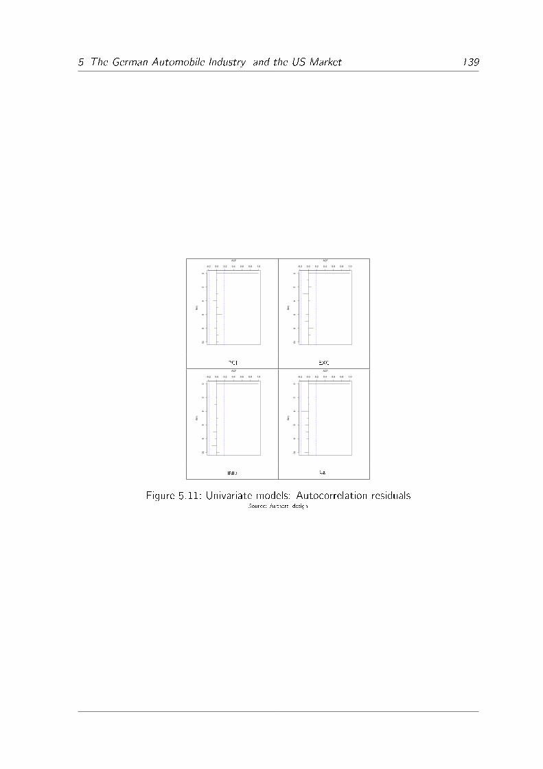
5 The German Automobile Industry and the US Market 139
02
46
810
-0.2 0.0 0.2 0.4 0.6 0.8 1.0
Lag
ACF
02
46
810
-0.2 0.0 0.2 0.4 0.6 0.8 1.0
Lag
ACF
PCI EXC
02
46
810
-0.2 0.0 0.2 0.4 0.6 0.8 1.0
Lag
ACF
02
46
810
-0.2 0.0 0.2 0.4 0.6 0.8 1.0
Lag
ACF
IND SAL
Figure 5.11: Univariate models: Autocorrelation residualsSource: Authors' design

5 The German Automobile Industry and the US Market 140
5.5 Cointegration and NN-VEC
In this section a NN-VEC including the three variables IND,SAL and EXC is constructed.
Afore in section 5.5.1 the cointegration relationship is calculated. In the subsequent
sections the NN-VEC including this cointegration relationship is estimated and used for
prediction. Via cross-validation it is also examined, how many hidden neurons should
be included in the model.
5.5.1 The Cointegration Relationship
The cointegration relationship is represented by a (3�1) vector B, which is transposed
and multiplied with the data vector. The output from this product is the stationary
univariate series zt . In general the existence of such a cointegration vector can be
explained by the fact that the e�ects of the non-stationary time series cancel each
other out. As OLS estimation did not result in any cointegration relationship, we use
the 2SLS method instead. Therefore a structural equation system is constructed using
the four variables IND,SAL, EXC and PCI:
INDt = b11 � SALt + b12 � EXCt + zt (5.5.1)
INDt = b21 � SALt + b22 � PCIt + ut (5.5.2)
The two equations can be interpreted as macroeconomic-environment (5.5.1) and
capital-market-incentive driven (5.5.2) supply-demand equation concerning the Ger-
man automobile industry production and the US market. IND and SAL are endogenous
variables, PCI and SAL are exogenous variables. Only equation (5.5.1) is used as coin-
tegration relationship in the following. This means, that the variable PCI is not directly
involved in the cointegration relationship. However it is needed, because only the si-
multaneous treatment of both equations ((5.5.1) and (5.5.2)) leads to a stationary
relationship in equation (5.5.1).
Both equations of the system are identi�ed. In the �rst step the variable SAL is regressed
on EXC and PCI. Subsequently in the second step IND is regressed on the estimated
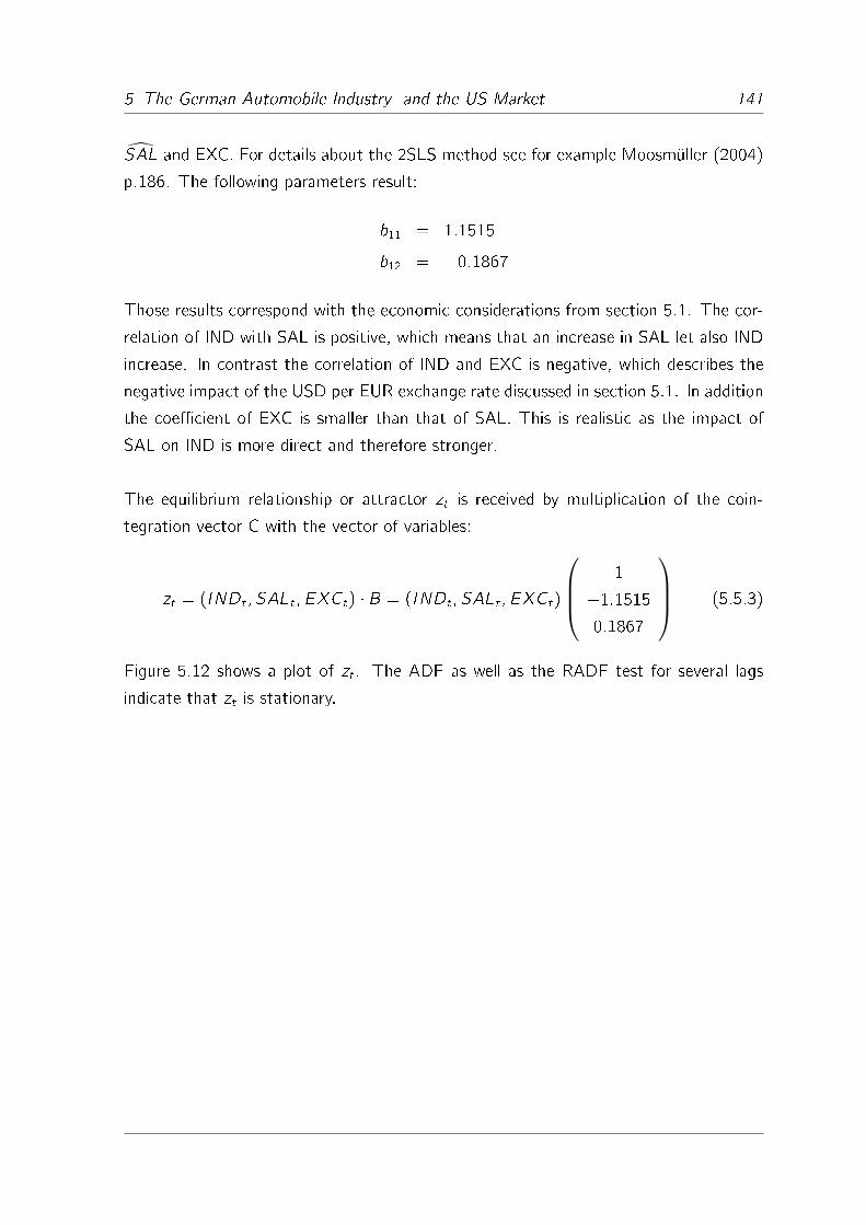
5 The German Automobile Industry and the US Market 141
SAL and EXC. For details about the 2SLS method see for example Moosmüller (2004)
p.186. The following parameters result:
b11 = 1:1515
b12 = �0:1867
Those results correspond with the economic considerations from section 5.1. The cor-
relation of IND with SAL is positive, which means that an increase in SAL let also IND
increase. In contrast the correlation of IND and EXC is negative, which describes the
negative impact of the USD per EUR exchange rate discussed in section 5.1. In addition
the coe�cient of EXC is smaller than that of SAL. This is realistic as the impact of
SAL on IND is more direct and therefore stronger.
The equilibrium relationship or attractor zt is received by multiplication of the coin-
tegration vector C with the vector of variables:
zt = (INDt ; SALt ; EXCt) � B = (INDt ; SALt ; EXCt)
1
�1:15150:1867
(5.5.3)
Figure 5.12 shows a plot of zt . The ADF as well as the RADF test for several lags
indicate that zt is stationary.

5 The German Automobile Industry and the US Market 142
0 20 40 60 80 100 120
-0.3
-0.2
-0.1
0.0
0.1
0.2
0.3
Time
Figure 5.12: Cointegration relationshipSource: Author's design

5 The German Automobile Industry and the US Market 143
5.5.2 Estimation of the NN-VEC
Before the NN-VEC can be estimated, the number of lags has to be determined for
the common model. We use lag order n=3 for the common model. The cointegration
relationship estimated in the previous section is used as zt . The NN-VEC is written in
vector representation (like equation (4.2.17)):�INDt
�EXCt
�SALt
=
3∑i=1
��i11 ��i12 ��i13��i21 ��i22 ��i23��i31 ��i32 ��i33
�INDt�i�SALt�i�EXCt�i
+
�01
�02
�03
+
�11
�21
�31
zt�1 +
h∑j=1
tanh
01j
02j
03j
+
11j
12j
13j
zt�1
�j +
"1t
"2t
"3t
This equation can be split into 3 independent equations with scalar outputs. This is
necessary for estimation. Initial values are uniformly setted equal to 0.05, � = 0:0001,
� = 100, �1 = 6 and �2 = 3. The maximum number of iterations is 11. Again the �rst
120 values are used for estimation, the last 8 values for prediction. Keeping the maxi-
mum number of iterations small helps to avoid the problem of overlearning here (which in
for univariate series is avoided by stopped training). Results for NN-VEC's with h=0,1,2
are shown in table 5.24 (results are calculated using the functions estimate.NNVEC()
in appendix B.10 and predict.NNVEC in appendix B.11). The table contains also a
linear VAR (estimated using the function VAR() in the package vars). Again one- and
eight step prediction is considered using the same performance measures as in section
5.4.2.
The results for the individual series concerning out-of-sample prediction vary with the
models in table 5.24. If we focus on the IND series, a NN-VEC(3) with h = 1 seems
to be the best model. With increasing h the prediction performance concerning the
IND series decreases. Results for the EXC series connected with that model are out-
performed by a model with linear cointegration, which again is not as good as the VAR
(one- and eight- step prediction). This let us assume that the EXC series is at least
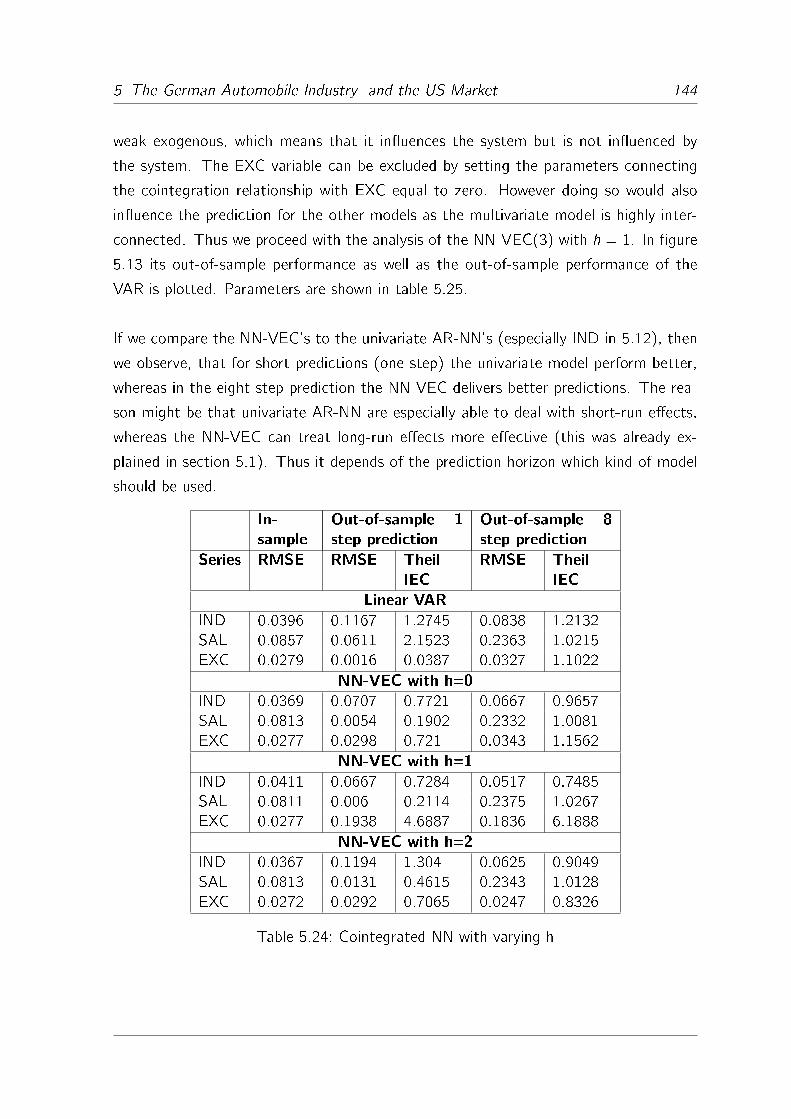
5 The German Automobile Industry and the US Market 144
weak exogenous, which means that it in�uences the system but is not in�uenced by
the system. The EXC variable can be excluded by setting the parameters connecting
the cointegration relationship with EXC equal to zero. However doing so would also
in�uence the prediction for the other models as the multivariate model is highly inter-
connected. Thus we proceed with the analysis of the NN-VEC(3) with h = 1. In �gure
5.13 its out-of-sample performance as well as the out-of-sample performance of the
VAR is plotted. Parameters are shown in table 5.25.
If we compare the NN-VEC's to the univariate AR-NN's (especially IND in 5.12), then
we observe, that for short predictions (one step) the univariate model perform better,
whereas in the eight step prediction the NN-VEC delivers better predictions. The rea-
son might be that univariate AR-NN are especially able to deal with short-run e�ects,
whereas the NN-VEC can treat long-run e�ects more e�ective (this was already ex-
plained in section 5.1). Thus it depends of the prediction horizon which kind of model
should be used.
In-
sample
Out-of-sample 1
step prediction
Out-of-sample 8
step prediction
Series RMSE RMSE Theil
IEC
RMSE Theil
IEC
Linear VAR
IND 0.0396 0.1167 1.2745 0.0838 1.2132
SAL 0.0857 0.0611 2.1523 0.2363 1.0215
EXC 0.0279 0.0016 0.0387 0.0327 1.1022
NN-VEC with h=0
IND 0.0369 0.0707 0.7721 0.0667 0.9657
SAL 0.0813 0.0054 0.1902 0.2332 1.0081
EXC 0.0277 0.0298 0.721 0.0343 1.1562
NN-VEC with h=1
IND 0.0411 0.0667 0.7284 0.0517 0.7485
SAL 0.0811 0.006 0.2114 0.2375 1.0267
EXC 0.0277 0.1938 4.6887 0.1836 6.1888
NN-VEC with h=2
IND 0.0367 0.1194 1.304 0.0625 0.9049
SAL 0.0813 0.0131 0.4615 0.2343 1.0128
EXC 0.0272 0.0292 0.7065 0.0247 0.8326
Table 5.24: Cointegrated NN with varying h
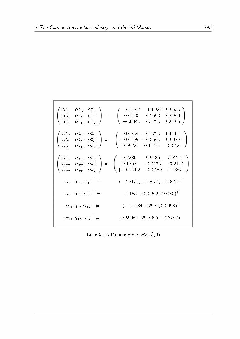
5 The German Automobile Industry and the US Market 145
��111 ��112 ��113��121 ��122 ��123��131 ��132 ��133
=
�0:3143 �0:0921 0:0526
0:0180 0:5500 0:0943
�0:0848 0:1295 0:0465
��211 ��212 ��213
��221 ��222 ��223��231 ��232 ��233
=
�0:0334 �0:1220 0:0161
�0:0605 �0:0546 0:0072
0:0522 0:1144 �0:0424
��311 ��312 ��313
��321 ��322 ��323��331 ��332 ��333
=
0:2236 0:5686 0:3274
0:1253 �0:0267 �0:2104]� 0:1702 �0:0480 0:0357
(�01; �02; �03)
> = (�0:9170;�5:9974;�5:9966)>
(�11; �12; �13)> = (0:1551; 12:2202; 2:9086)>
( 01; 02; 03)> = (�4:1134; 0:2569; 0:0098)>
( 11; 12; 13)> = (0:6906;�29:7890;�4:3797)>
Table 5.25: Parameters NN-VEC(3)
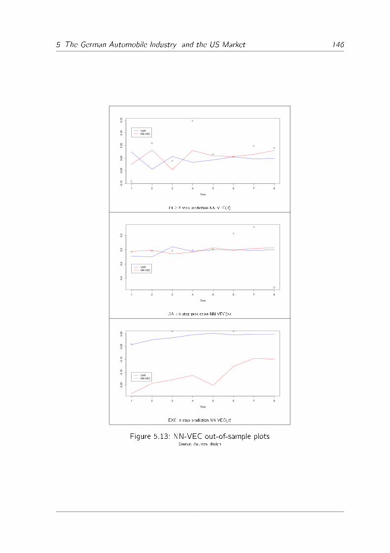
5 The German Automobile Industry and the US Market 146
1 2 3 4 5 6 7 8
-0.10
-0.05
0.00
0.05
0.10
0.15
Time
VARNN-VEC
IND: 8 step prediction NN-VEC(3)
1 2 3 4 5 6 7 8
-0.4
-0.2
0.0
0.2
Time
VARNN-VEC
SAL: 8 step prediction NN-VEC(3)
1 2 3 4 5 6 7 8
-0.20
-0.15
-0.10
-0.05
0.00
Time
VARNN-VEC
EXC: 8 step prediction NN-VEC(3)
Figure 5.13: NN-VEC out-of-sample plotsSource: Authors' design

5 The German Automobile Industry and the US Market 147
5.5.3 Residual Analysis
Again like in section 5.4.4 the assumptions on the residuals are checked. Therefore the
same methods are used. Residuals of the IND and SAL series seem to �t at the i.i.d.
Gaussian WN assumption, whereas the residuals of the EXC series does not. Conse-
quently the model could be estimated again with di�erent settings for the algorithm.
Alternatively the EXC series could be excluded from the cointegration relationship.
-0.10 -0.05 0.00 0.05 0.10
02
46
810
12
-0.2 -0.1 0.0 0.1 0.2
01
23
45
6
IND SAL
0.0 0.1 0.2 0.3 0.4 0.5
02
46
810
12
EXC
Figure 5.14: Histogram residuals NN-VEC(3)Source: Authors' design
Series Mean � Skewness Kurtosis
IND 0.0000 0.0362 -0.2181 0.2999
SAL 0.0000 0.0814 -0.0144 -0.2025
EXC 0.0547 0.0782 2.7748 10.6639
Table 5.26: NN-VEC(3): Skewness and kurtosis
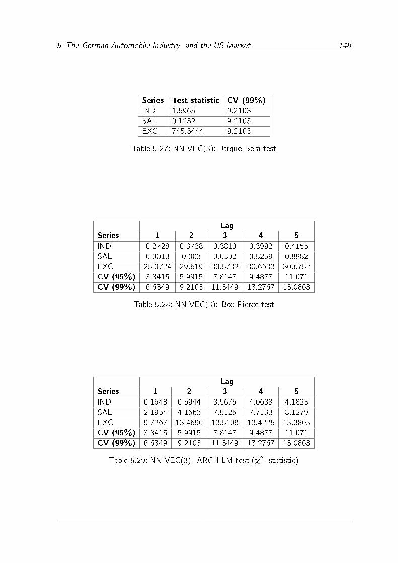
5 The German Automobile Industry and the US Market 148
Series Test statistic CV (99%)
IND 1.5965 9.2103
SAL 0.1232 9.2103
EXC 745.3444 9.2103
Table 5.27: NN-VEC(3): Jarque-Bera test
Lag
Series 1 2 3 4 5
IND 0.2728 0.3738 0.3810 0.3992 0.4155
SAL 0.0013 0.003 0.0592 0.5259 0.8982
EXC 25.0724 29.619 30.5732 30.6633 30.6752
CV (95%) 3.8415 5.9915 7.8147 9.4877 11.071
CV (99%) 6.6349 9.2103 11.3449 13.2767 15.0863
Table 5.28: NN-VEC(3): Box-Pierce test
Lag
Series 1 2 3 4 5
IND 0.1648 0.5944 3.5675 4.0638 4.1823
SAL 2.1954 4.1663 7.5125 7.7133 8.1279
EXC 9.7267 13.4696 13.5108 13.4225 13.3803
CV (95%) 3.8415 5.9915 7.8147 9.4877 11.071
CV (99%) 6.6349 9.2103 11.3449 13.2767 15.0863
Table 5.29: NN-VEC(3): ARCH-LM test (�2- statistic)
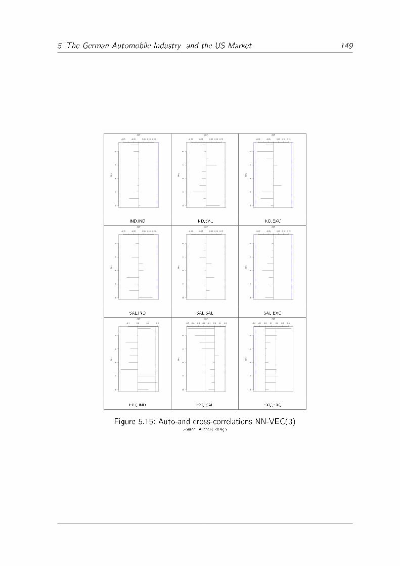
5 The German Automobile Industry and the US Market 149
24
68
10
-0.15 -0.05 0.05 0.10 0.15
Lag
ACF
24
68
10
-0.15 -0.05 0.05 0.10 0.15
Lag
ACF
24
68
10
-0.15 -0.05 0.05 0.10 0.15
Lag
ACF
IND,IND IND,SAL IND,EXC
24
68
10
-0.15 -0.05 0.05 0.10 0.15
Lag
ACF
24
68
10
-0.15 -0.05 0.05 0.10 0.15
Lag
ACF
24
68
10
-0.15 -0.05 0.05 0.10 0.15
Lag
ACF
SAL,IND SAL,SAL SAL,EXC
24
68
10
-0.1 0.0 0.1 0.2
Lag
ACF
24
68
10
-0.5 -0.4 -0.3 -0.2 -0.1 0.0 0.1 0.2
Lag
ACF
24
68
10
-0.2 -0.1 0.0 0.1 0.2 0.3 0.4
Lag
ACF
EXC,IND EXC,SAL EXC,EXC
Figure 5.15: Auto-and cross-correlations NN-VEC(3)Source: Authors' design

6 Conclusion 150
6 Conclusion
In this dissertation a method for analysis and prediction of nonlinear time series, AR-NN,
based on neural networks is discussed. Nonlinear time series methods have to be applied,
if any nonlinear e�ects or nonstandard features are in the data, which would disturb
linear methods. Such e�ects occur especially with economic crises as it is shown in the
empirical part. AR-NN combine the properties parametric and universal approximation,
which makes them applicable at any nonlinear e�ect, as well as easily handable concern-
ing model validation and parameter tests. Alternative models, in contrast, are either
nonparametric ( kernel regression) or dedicated to special nonlinearities like structural
breaks (threshold regression). In the empirical part it is shown, that AR-NN outperform
many linear and nonlinear methods concerning out-of-sample prediction, particularly in
one-step prediction.
Further AR-NN are extended to multivariate error correction models based on the er-
ror correction theorem of Escribano and Mira (2002). This model combines a linear
long-run equilibrium with nonlinear adjustment. If some linearly cointegrated series are
nonlinear, such nonlinear error correction is essential. The linear cointegration rela-
tionship is estimated using a structural model and the 2SLS estimation method. This
means that time series analysis here is combined with structural equation models. This
is not yet very common in literature but might be an interesting point of research. The
NN-VEC as proposed here, combined with structural equations, are especially useful
for prediction of time series involved in a supply-demand system. The example in the
empirical part is such a system, whereas the demand for foreign cars in the USA, the
industry production of the car manufacturing industry in Germany (corresponds to sup-
ply) and the USD/EUR exchange rate are examined.
Various methods from existing literature for data preparation, variable selection, model
estimation and models validation are brought together here with neural network the-
ory to provide an adequate toolkit for our AR-NN models. Therefore some of those
methods are modi�ed, especially the MIC in combination with the method of Hausser
and Strimmer (2009) or the early stopping method, which is extended for a search of

6 Conclusion 151
a global minimum within a �nite number of iterations. In this �eld no theory exists
in literature about multivariate neural networks, thus VAR-NN and NN-VEC are newly
introduced by this dissertation.
Future topics of research based on this dissertation might be a comprehensive study
about nonlinearities and economic crises, which would include data from various �elds
of economics including crises (�nancial data as stock indices as well as macroeconomic
data as growth of GDP). The aim of such a study should be to show if crises cause
nonlinearities in the data. The statistical tool therefore can be the nonlinearity test
of Teräsvirta, Lin and Granger (1993). Furthermore the NN-VEC can be extended to
a model which includes a nonlinear cointegration relationship. Although such a model
might be more complex than the one in this dissertation, it might be possible to include
a broader range of cointegration relationships and provide better predictions for vari-
ables which are only nonlinear cointegrated. Finally, the comparison between the models
from this dissertation and linear as well as nonlinear alternatives could be continued,
using other data sets from various �elds of application, especially to see if there is any
supply-demand relationship.

A Proof of Theorem 2.1 152
A Proof of Theorem 2.1
For this proof see Hornik (1993) p.1071. At �rst let us give a short nonformal de-
scription of the proof: We de�ne a subset of G(;B;W) such that W contains a
neighborhood of the origin and B is compact and nondegenerate (see the requirements
concerning those intervals in theorem 2.1) and make use of an extension of the dual-
space argument of Cybenko (1989), which says that, if the selected subset should not
be dense in F(X), a certain nonzero measure may exist. We show that no such measure
exists for any selected subset of G(;B;W) and thus proofe theorem.
Let Xt�1 be a nondegenerate compact interval, Xt�1 � Rn. j � j denotes the determi-
nant. The �- neighborhood of is denoted by X� = fS : jS �Xt�1j � � for Xt�1 2 Xg.Let W (Xt�1) be a function on the interval [�1; 1],
W (Xt�1) =
c � e� 1
1�jXt�1j2 jXt�1j < 1
0 jXt�1j � 1:(A.0.1)
where c is to choose such that∫
Rn W (Xt�1)dXt�1 = 1. With �0 > 0 we can formulate
the �-molli�er of ,
J�(Xt�1) =
∫jUj�1
W (U)(Xt�1 � �U)dU: (A.0.2)
Concerning the molli�er the following fact holds, that if is Riemann integrable on
X�, then it is possible to approximate J� uniformly on X by linear combinations of
functions (Xt�1 � S) for jSj � �. (See lemma 4 in Hornik (1993) p.1070).
Let the vector M = maxfjXt�1j : Xt�1 2 Xg. Choose the initial sets W0, B0 and
some numbers �0 and �0 such that W0 = f� : j� j < �0g � W and B�0M+�00 � B.
Further should be nonpolynomial on W0. According to the dual space argument, if
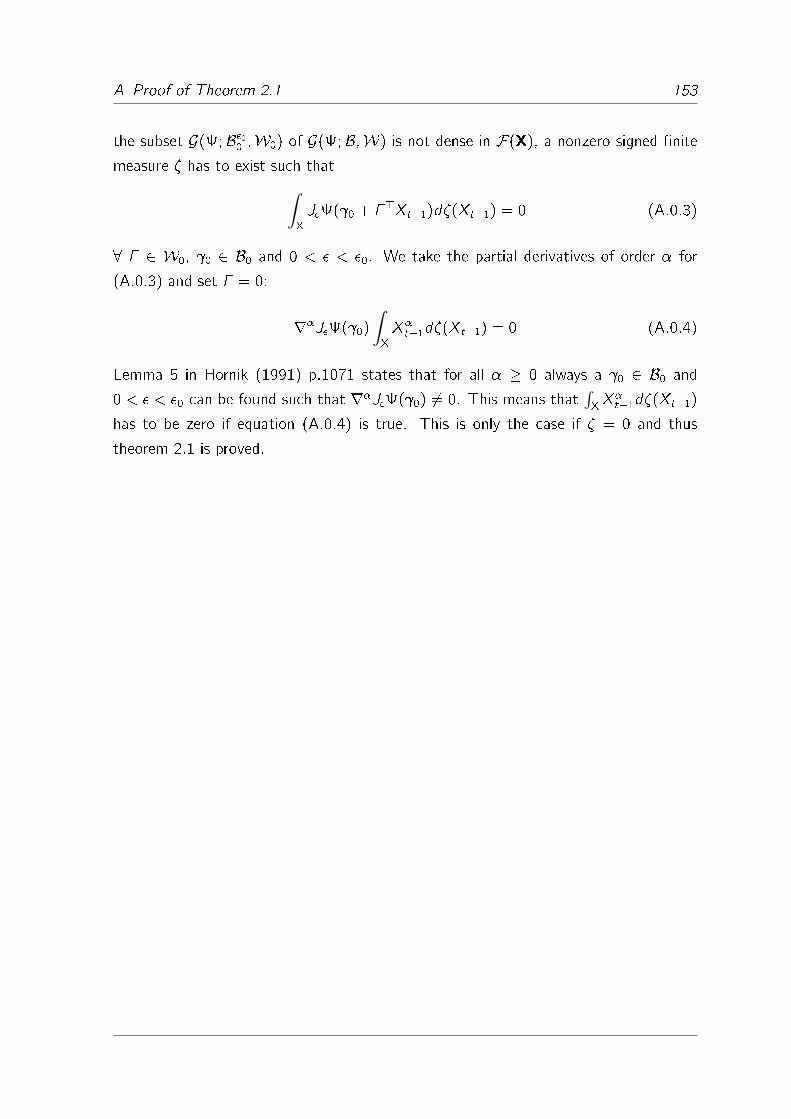
A Proof of Theorem 2.1 153
the subset G(;B�00 ;W0) of G(;B;W) is not dense in F(X), a nonzero signed �nite
measure � has to exist such that∫X
J�( 0 + �>Xt�1)d�(Xt�1) = 0 (A.0.3)
8 � 2 W0, 0 2 B0 and 0 < � < �0. We take the partial derivatives of order � for
(A.0.3) and set � = 0:
r�J�( 0)
∫X
X�t�1d�(Xt�1) = 0 (A.0.4)
Lemma 5 in Hornik (1991) p.1071 states that for all � � 0 always a 0 2 B0 and
0 < � < �0 can be found such that r�J�( 0) 6= 0. This means that∫XX�t�1d�(Xt�1)
has to be zero if equation (A.0.4) is true. This is only the case if � = 0 and thus
theorem 2.1 is proved.
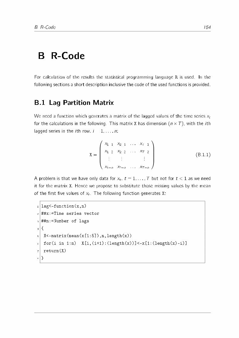
B R-Code 154
B R-Code
For calculation of the results the statistical programming language R is used. In the
following sections a short description inclusive the code of the used functions is provided.
B.1 Lag Partition Matrix
We need a function which generates a matrix of the lagged values of the time series xt
for the calculations in the following. This matrix X has dimension (n� T ), with the ith
lagged series in the ith row, i = 1; : : : ; n:
X =
x1�1 x2�1 : : : xT�1
x1�2 x2�2 : : : xT�2
......
...
x1�n x2�n : : : xT�n
(B.1.1)
A problem is that we have only data for xt , t = 1; : : : ; T but not for t < 1 as we need
it for the matrix X. Hence we propose to substitute those missing values by the mean
of the �rst �ve values of xt . The following function generates X:
1 lag<-function(x,n)
2 ##x:=Time series vector
3 ##n:=Number of lags
4 {
5 X<-matrix(mean(x[1:5]),n,length(x))
6 for(i in 1:n) X[i,(i+1):(length(x))]<-x[1:(length(x)-i)]
7 return(X)
8 }
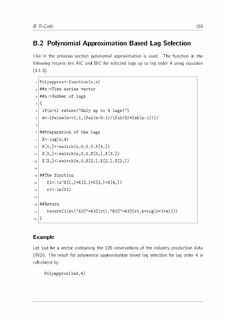
B R-Code 155
B.2 Polynomial Approximation Based Lag Selection
Like in the previous section polynomial approximation is used. The function in the
following returns the AIC and BIC for selected lags up to lag order 4 using equation
(3.1.3).
1 Polyapprox<-function(x,n)
2 ##x:=Time series vector
3 ##n:=Number of lags
4 {
5 if(n>4) return("Only up to 4 lags!")
6 m<-ifelse(n==1,1,(fak(n+3-1)/(fak(3)*fak(n-1))))
7
8 ##Preparation of the lags
9 X<-lag(x,4)
10 X[4,]<-switch(n,0,0,0,X[4,])
11 X[3,]<-switch(n,0,0,X[3,],X[3,])
12 X[2,]<-switch(n,0,X[2,],X[2,],X[2,])
13
14 ##The function
15 f1<-(x~X[1,]*X[2,]*X[3,]*X[4,])
16 r1<-lm(f1)
17
18 ##Return
19 return(list("AIC"=AIC(r1),"BIC"=AIC(r1,k=log(n+1+m))))
20 }
Example
Let ind be a vector containing the 128 observations of the industry production data
(IND). The result for polynomial approximation based lag selection for lag order 4 is
calculated by
Polyapprox(ind,4)
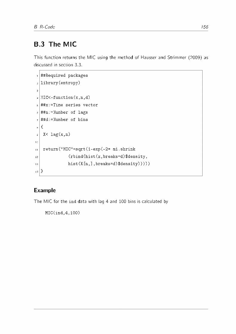
B R-Code 156
B.3 The MIC
This function returns the MIC using the method of Hausser and Strimmer (2009) as
discussed in section 3.3.
1 ##Required packages
2 library(entropy)
3
4 MIC<-function(x,n,d)
5 ##x:=Time series vector
6 ##n:=Number of lags
7 ##d:=Number of bins
8 {
9 X<-lag(x,n)
10
11 return("MIC"=sqrt(1-exp(-2* mi.shrink
12 (rbind(hist(x,breaks=d)$density,
13 hist(X[n,],breaks=d)$density)))))
14 }
Example
The MIC for the ind data with lag 4 and 100 bins is calculated by
MIC(ind,4,100)
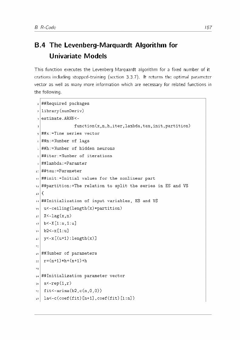
B R-Code 157
B.4 The Levenberg-Marquardt Algorithm for
Univariate Models
This function executes the Levenberg-Marquardt algorithm for a �xed number of it-
erations including stopped-training (section 3.3.7). It returns the optimal parameter
vector as well as many more information which are necessary for related functions in
the following.
1 ##Required packages
2 library(numDeriv)
3 estimate.ARNN<-
4 function(x,n,h,iter,lambda,tau,init,partition)
5 ##x:=Time series vector
6 ##n:=Number of lags
7 ##h:=Number of hidden neurons
8 ##iter:=Number of iterations
9 ##lambda:=Paramter
10 ##tau:=Parameter
11 ##init:=Initial values for the nonlinear part
12 ##partition:=The relation to split the series in ES and VS
13 {
14 ##Initialization of input variables, ES and VS
15 u<-ceiling(length(x)*partition)
16 X<-lag(x,n)
17 b<-X[1:n,1:u]
18 b2<-x[1:u]
19 y<-x[(u+1):length(x)]
20
21 ##Number of parameters
22 r=(n+1)*h+(n+1)+h
23
24 ##Initialization parameter vector
25 a<-rep(1,r)
26 fit<-arima(b2,c(n,0,0))
27 la<-c(coef(fit)[n+1],coef(fit)[1:n])

B R-Code 158
28 a<-c(la,rep(init,(r-n-1)))
29 neu<-a
30
31 ##Initialization internal storage
32 h1<-matrix(NA,(iter+1),length(a))
33 h2<-matrix(NA,(iter+1),length(y))
34 v1<-rep(NA,(iter+1))
35 v2<-rep(NA,(iter+1))
36
37 ##Constructs for internal usage
38 pv<-rep(NA,length(y))
39 c<-rep(NA,n)
40 e2<-0
41 s1<-0
42 if(h>0)
43 {
44 q=0
45 s1<-rep(NA,h)
46 s1[1]<-(n+2)
47 if(h>1) for(i in 2:h) s1[i]<-(s1[i-1]+(n+2))
48
49 ##Basic components of functions
50 e2<-expression(for(i in s1)
51 {
52 +(tanh(crossprod(b,a[i:(i+n-1)])
53 +a[i+n]))*a[i+n+1]
54 })
55 }
56 e1<-expression(a[1]+crossprod(b,a[2:(n+1)]))
57
58 ##General functions
59 f<-function(s1,a) eval(e1)+eval(e2)
60 ff<-function(a) eval(e1)
61

B R-Code 159
62 ##Function with respect to the network weights
63 f1<-function(a) eval(e1)+eval(e2)
64
65 ##Difference between real and estimated values
66 f2<-function(a) b2-f1(a)
67
68 ##Performance function
69 f3<-function(a) sum((f2(a))^2)
70
71 ##Function for prediction
72 f4<-function(a,b) eval(e1)+eval(e2)
73
74 ##Execution of the algorithm
75 for(i in 1:(iter+1))
76 {
77 m1<-c(b2[(length(b2)-n+1):length(b2)],pv)
78 for(j in 1:length(y))
79 {
80 m1[j+n]<-f4(a,m1[(j+n-1):(j)])[1]
81 }
82 v1[i]<-(f3(a))
83 v2[i]<-sum((y-m1[(n+1):(length(m1))])^2)
84 h1[i,1:(length(a))]<-a
85 h2[i,1:(length(y))]<-m1[(n+1):(length(m1))]
86 i=i+1
87 if(f3(neu)==f3(a))
88 {
89 t=1
90 }
91 else
92 {
93 if(f3(neu)<(f3(a))
94 {
95 t=tau
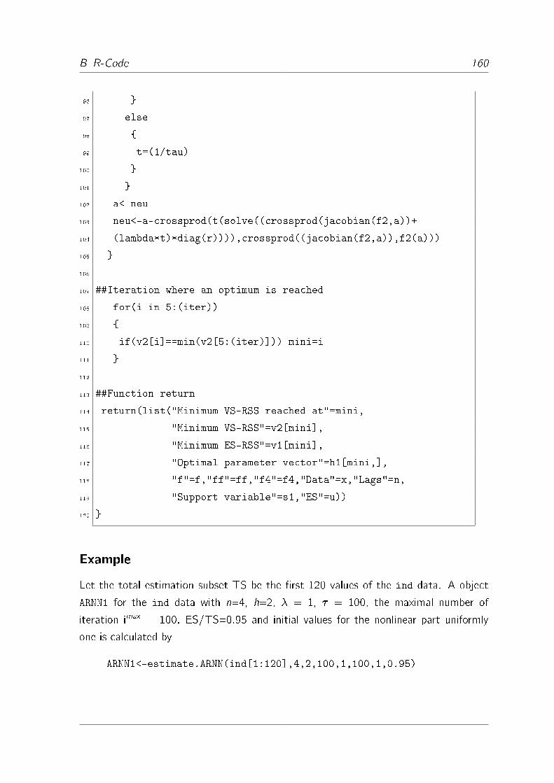
B R-Code 160
96 }
97 else
98 {
99 t=(1/tau)
100 }
101 }
102 a<-neu
103 neu<-a-crossprod(t(solve((crossprod(jacobian(f2,a))+
104 (lambda*t)*diag(r)))),crossprod((jacobian(f2,a)),f2(a)))
105 }
106
107 ##Iteration where an optimum is reached
108 for(i in 5:(iter))
109 {
110 if(v2[i]==min(v2[5:(iter)])) mini=i
111 }
112
113 ##Function return
114 return(list("Minimum VS-RSS reached at"=mini,
115 "Minimum VS-RSS"=v2[mini],
116 "Minimum ES-RSS"=v1[mini],
117 "Optimal parameter vector"=h1[mini,],
118 "f"=f,"ff"=ff,"f4"=f4,"Data"=x,"Lags"=n,
119 "Support variable"=s1,"ES"=u))
120 }
Example
Let the total estimation subset TS be the �rst 120 values of the ind data. A object
ARNN1 for the ind data with n=4, h=2, � = 1, � = 100, the maximal number of
iteration imax = 100, ES/TS=0.95 and initial values for the nonlinear part uniformly
one is calculated by
ARNN1<-estimate.ARNN(ind[1:120],4,2,100,1,100,1,0.95)

B R-Code 161
B.5 Residuals ES
This function returns the residuals of an estimated AR-NN (only ES residuals).
1 residuals.ARNN<-function(l)
2 ##l:=Result generated by function estimate.ARNN
3 {
4 return(l$"Data"[1:l$"ES"]-l$"f"(l$"Support variable",
5 l$"Optimal parameter vector"))
6 }
Example
ES-residuals for the object ARNN1 are calculated by
residuals.ARNN(ARNN1)
The in-sample RMSE is calculated by
sqrt(sum((residuals.ARNN(ARNN1))^2)/(120*0.95))
B R-Code 162
B.6 Fitted Values ES
This function returns the �tted values of an estimated AR-NN (only ES �tted values).
1 fitted.ARNN<-function(l)
2 ##l:=Result generated by function estimate.ARNN
3 {
4 return(l$"f"(l$"Support variable",l$"Optimal parameter vector"))
5 }
Example
ES-�tted values for the object ARNN1 are calculated by
fitted.ARNN(ARNN1)
B R-Code 163
B.7 Prediction
This function returns one- and more-step predictions for an estimated AR-NN.
1 predict.ARNN<-function(l,k)
2 ##l:=Result generated by function estimate.ARNN
3 ##k:=Steps to predict
4 {
5 c<-rep(NA,n)
6 a<-l$"Optimal parameter vector"
7 n<-l$"Lags"
8 m<-c(l$"Data"[(length(l$"Data")-n+1):
9 length(l$"Data")],rep(NA,k))
10
11 for(j in 1:k) m[j+n]<-l$"f4"(a,m[(j+n-1):j])
12
13 return(m[(n+1):(length(m))])
14 }
Example
An one-step prediction out of the object ARNN1 is calculated by
predict.ARNN(ARNN1,1)

B R-Code 164
B.8 The Covariance Matrix
This function returns the NIC, the Wald test statistics for each parameter or the co-
variance matrix of an estimated AR-NN.
1 covariance.ARNN
2 <-function(l,h,type=c("NIC","Wald","Covariance"))
3 ##l:=Result generated by function estimate.ARNN
4 ##h:=Number of hidden neurons
5 {
6 ##Input elements
7 x<-l$"Data"[1:l$"ES"]
8 n<-l$"Lags"
9 r=(n+1)*h+(n+1)+h
10 a<-l$"Optimal parameter vector"[1:r]
11
12 ##Network function
13 if(h>0)
14 {
15 s1<-l$"Support variable"[1:h]
16 f<-expression(l1$"f"(s1,a))
17 f1<-function(a) eval(f)
18 }
19 else
20 {
21 f1<-l$"ff"
22 }
23
24 ##RSS function
25 f2<-function(a) 0.5*sum((x-f1(a)[1:l$"ES"])^2)
26
27 ##Submatrices
28 Gamma<-function(a)
29 (1/length(x))*hessian(f2,a)
30 Upsilon<-function(a)

B R-Code 165
31 (1/length(x))*(grad(f2,a)%*%t(grad(f2,a)))
32
33 ##Covariance matrix
34 C<-Upsilon(a)%*%solve(Gamma(a))%*%Upsilon(a)
35
36 Wald<-a^2/diag(C)
37
38 NIC<-(1/length(x))*(f2(a)+(1/length(x))
39 *sum(diag(Upsilon(a)%*%solve(Gamma(a)))))
40
41 ##Return
42 if(type=="Wald")
43 {
44 return(list("Wald statstic"=Wald))
45 }
46 if(type=="NIC")
47 {
48 return(list("NIC"=NIC))
49 }
50 if(type=="Covariance")
51 {
52 return(list("Covariance matrix"=C))
53 }
54 }
Example
The NIC for the object ARNN1 is calculated by
covariance.ARNN(ARNN1,2,type="NIC")
B R-Code 166
B.9 The Lee-White-Granger Test
This function executes the Lee-White-Granger test for additional hidden nonlinearity
(see section 3.4.1.1 and Lee, White and Granger (1993)).
1 LWG.test<-function(l)
2 ##l:=Result generated by function estimate.ARNN
3 {
4 ##Preparation of the lagged matrix
5 n<-l$"Lags"
6 x<-l$"Data"[1:(length(l$"Data")*l$"ES/TS")]
7 X<-lag(x,n)
8 a<-l$"Optimal parameter vector"
9 f1<-l$"f1"
10
11 ##Number of paramters
12 m<-ifelse(n==1,1,(fak(n+3)/(fak(3)*fak(n))-n-1))
13
14 ##Preparation of the input for the polynomial term
15 Y<-lag(x,4)
16 Y[4,]<-switch(n,0,0,0,Y[4,])
17 Y[3,]<-switch(n,0,0,Y[3,],Y[3,])
18 Y[2,]<-switch(n,0,Y[2,],Y[2,],Y[2,])
19
20 ##Residuals of the restricted function
21 r1<-x-f1(a)
22
23 ##Residuals of the unrestricted function
24 f2<-(r1~jacobian(f1,a)+Y[1,]*Y[2,]*Y[3,]+Y[4,])
25 r2<-lm(f2)
26
27 ##The test statistics
28 T1<-length(x)*(sum(fitted(r2))^2
29 /sum((r1)^2))
30 T2<-((sum((r1)^2)-sum((residuals(r2))^2))/m)/

B R-Code 167
31 (sum((residuals(r2))^2)/(length(x)-n-m))
32
33 ##Return
34 return(list("Chi-square statistic"=
35 c("Test statistic"=T1,"df"=m, "Critical value"
36 =qchisq(0.95,m)),"F statistic"=c("Test statistic"
37 =T2,"df1"=m,"df2"=(length(x)-n-m),"Critical
38 value"=qf(0.95,df1=m,df2=(length(x)-n-m)))))
39 }
Example
The Lee-White-Granger test statstic for the object ARNN1 is calculated by
LWG.test(ARNN1)
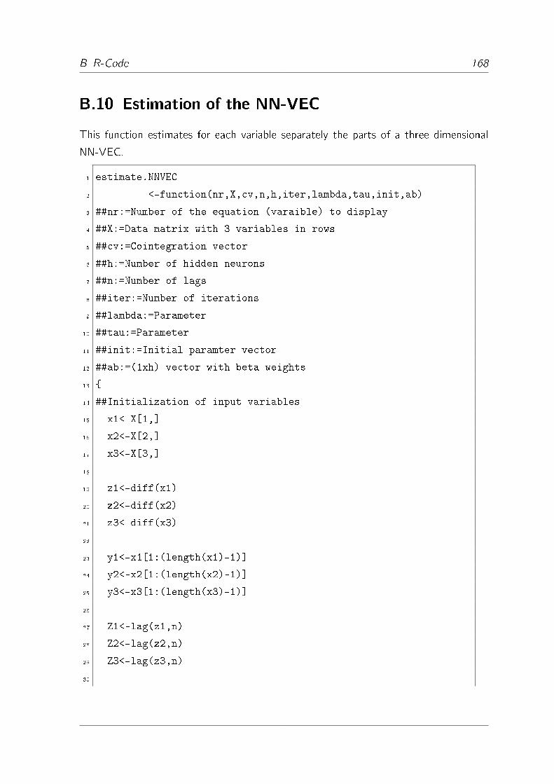
B R-Code 168
B.10 Estimation of the NN-VEC
This function estimates for each variable separately the parts of a three dimensional
NN-VEC.
1 estimate.NNVEC
2 <-function(nr,X,cv,n,h,iter,lambda,tau,init,ab)
3 ##nr:=Number of the equation (varaible) to display
4 ##X:=Data matrix with 3 variables in rows
5 ##cv:=Cointegration vector
6 ##h:=Number of hidden neurons
7 ##n:=Number of lags
8 ##iter:=Number of iterations
9 ##lambda:=Parameter
10 ##tau:=Parameter
11 ##init:=Initial paramter vector
12 ##ab:=(1xh) vector with beta weights
13 {
14 ##Initialization of input variables
15 x1<-X[1,]
16 x2<-X[2,]
17 x3<-X[3,]
18
19 z1<-diff(x1)
20 z2<-diff(x2)
21 z3<-diff(x3)
22
23 y1<-x1[1:(length(x1)-1)]
24 y2<-x2[1:(length(x2)-1)]
25 y3<-x3[1:(length(x3)-1)]
26
27 Z1<-lag(z1,n)
28 Z2<-lag(z2,n)
29 Z3<-lag(z3,n)
30

B R-Code 169
31 b<-rbind(Z1,Z2,Z3)
32 bb<-rbind(y1,y2,y3)
33
34 b2<-diff(X[nr,])
35
36 ##Number of parameters
37 r=2*h+2+n*3
38
39 ##Initialization parameter vector
40 a<-t(matrix(init,1,r))
41 neu<-a
42
43 ##Initialization internal constructs
44 s<-c(1,3,5,7)
45 ak<-c(ab[1],0,ab[2],0,ab[3],0,ab[4])
46
47 ##Basics for network functions
48 e1<-expression(
49 t(b)%*%a[1:(n*3),]+
50 a[n*3+1,]+t(a[n*3+2,]%*%(cv%*%bb))+
51 for(i in 1:s[h])
52 {
53 +tanh(a[n*3+2+i,]+
54 t(a[n*3+3+i,]%*%(cv%*%bb)))*ak[i]
55 })
56
57 e2<-expression(
58 t(b)%*%a[1:(n*3),]+
59 a[n*3+1,]+t(a[n*3+2,]%*%(cv%*%bb)))
60
61 e<-ifelse(h>0,e1,e2)
62
63 ##Definition network function respective the weights
64 f1<-function(a) eval(e)

B R-Code 170
65
66 ##Difference between real and estimated values
67 f2<-function(a) b2-f1(a)
68
69 ##Performance function
70 f3<-function(a) sum((f2(a))^2)
71
72 ##Execution of the algorithm
73 for(i in 1:(iter+1))
74 {
75 i=i+1
76 t<-ifelse(f3(neu)>=f3(a),tau,(1/tau))
77 a<-neu
78 neu<-a-crossprod(t(solve((crossprod
79 (jacobian(f2,a))+(lambda*t)*diag(r)))),
80 crossprod((jacobian(f2,a)),f2(a)))
81 }
82
83 ##Return
84 return(list("Minimal RSS"=f3(neu),
85 "Optimal parameter vector"=neu,
86 "f"=function(a,b,bb,g) eval(e),"Cointegration relationship"
87 =cv,"Beta vector"=ak,"DiffData"=b,"LevelData"=bb,
88 "Lags"=n,"Support variable"=s,"Residuals"=f2(neu)))
89 }
Example
Again the TS contains 120 values. Let the cointegration vector be (1;�1:1515; 0:1867)>and the �-values �1 ==6, �2=3, �3 = 1:5, �4 = 0:1. Objects NNVEC1, NNVEC2
and NNVEC3 for the three series using separate equations (like equation (4.2.15) and
(4.2.16)) with n=2, h=4, � = 0:0001, � = 100, the maximal number of iteration
imax = 11, and initial values uniformly 0.05 are calculated by
X<-rbind(ind[1:120],sal[1:120],exc[1:120])

B R-Code 171
cv<-c(1,-1.1515,0.1867)
ab<-c(6,3,1.5,0.1)
NNVEC1<-estimate.NNVEC(1,X,cv,2,4,100,0.0001,100,0.05,ab)
NNVEC2<-estimate.NNVEC(2,X,cv,2,4,100,0.0001,100,0.05,ab)
NNVEC3<-estimate.NNVEC(3,X,cv,2,4,100,0.0001,100,0.05,ab)
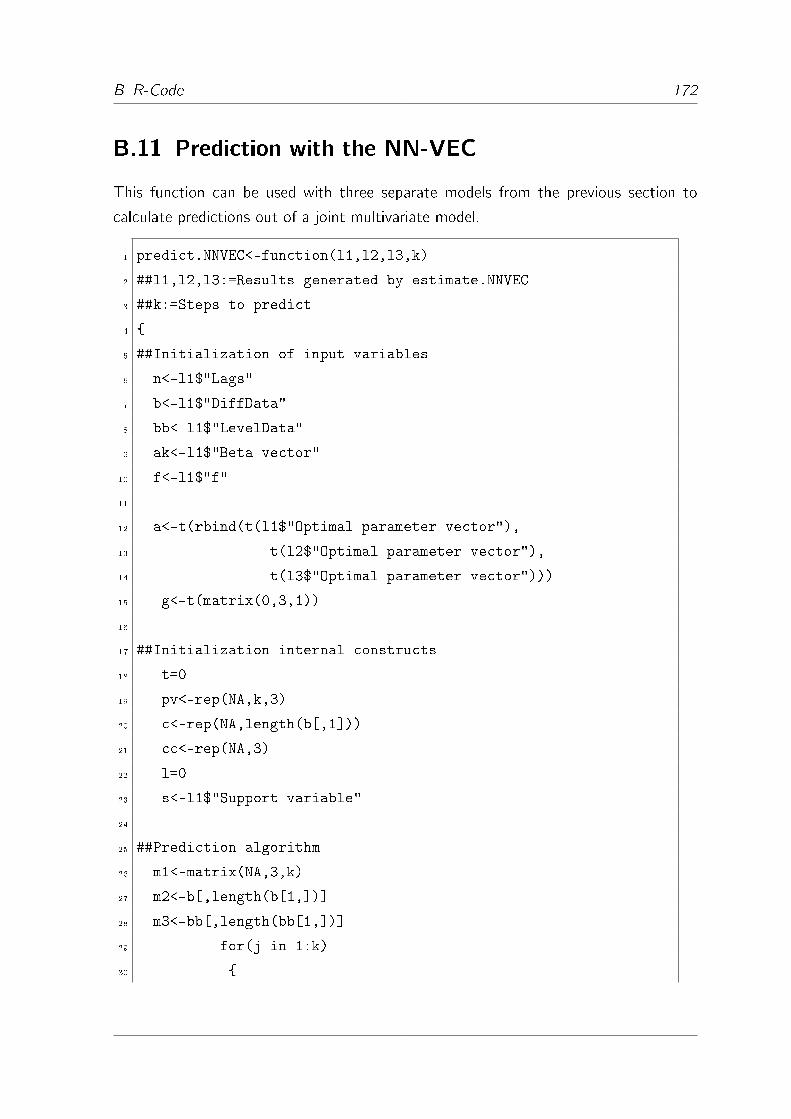
B R-Code 172
B.11 Prediction with the NN-VEC
This function can be used with three separate models from the previous section to
calculate predictions out of a joint multivariate model.
1 predict.NNVEC<-function(l1,l2,l3,k)
2 ##l1,l2,l3:=Results generated by estimate.NNVEC
3 ##k:=Steps to predict
4 {
5 ##Initialization of input variables
6 n<-l1$"Lags"
7 b<-l1$"DiffData"
8 bb<-l1$"LevelData"
9 ak<-l1$"Beta vector"
10 f<-l1$"f"
11
12 a<-t(rbind(t(l1$"Optimal parameter vector"),
13 t(l2$"Optimal parameter vector"),
14 t(l3$"Optimal parameter vector")))
15 g<-t(matrix(0,3,1))
16
17 ##Initialization internal constructs
18 t=0
19 pv<-rep(NA,k,3)
20 c<-rep(NA,length(b[,1]))
21 cc<-rep(NA,3)
22 l=0
23 s<-l1$"Support variable"
24
25 ##Prediction algorithm
26 m1<-matrix(NA,3,k)
27 m2<-b[,length(b[1,])]
28 m3<-bb[,length(bb[1,])]
29 for(j in 1:k)
30 {
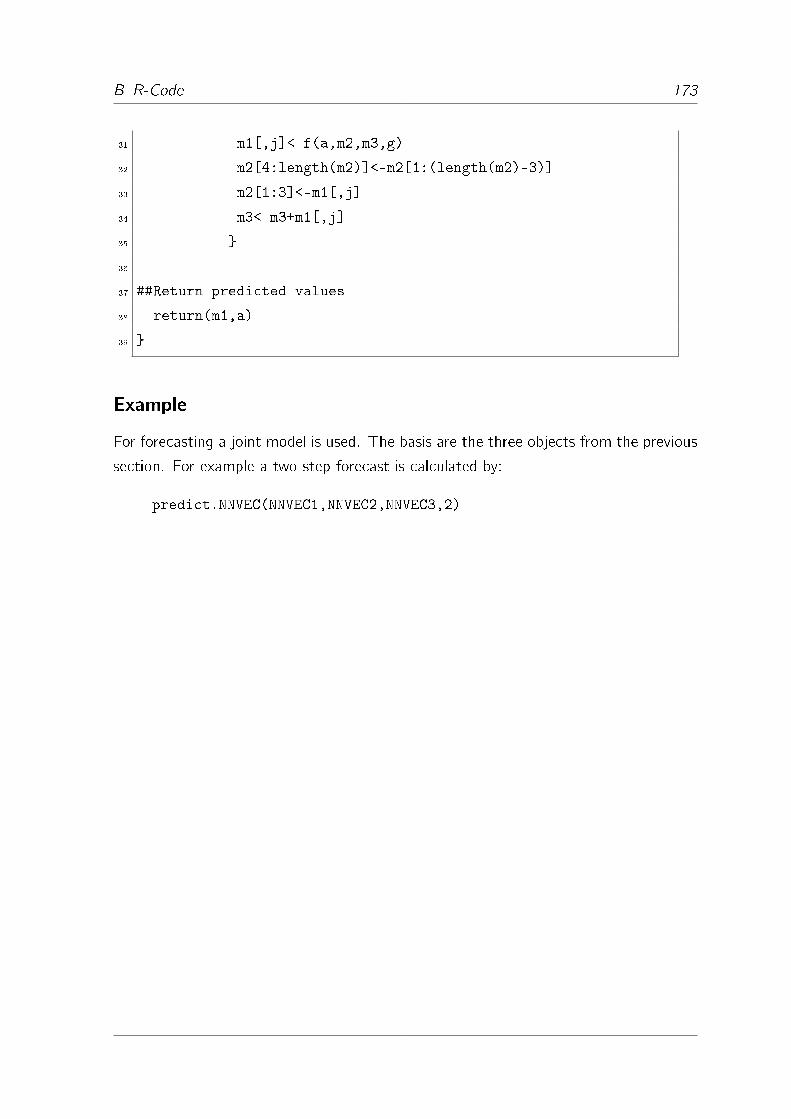
B R-Code 173
31 m1[,j]<-f(a,m2,m3,g)
32 m2[4:length(m2)]<-m2[1:(length(m2)-3)]
33 m2[1:3]<-m1[,j]
34 m3<-m3+m1[,j]
35 }
36
37 ##Return predicted values
38 return(m1,a)
39 }
Example
For forecasting a joint model is used. The basis are the three objects from the previous
section. For example a two step forecast is calculated by:
predict.NNVEC(NNVEC1,NNVEC2,NNVEC3,2)

Bibliography 174
Bibliography
Akaike, H. (1974): A New Look at the Statistical Model Identi�cation in: IEEE Trans-
actions on Automatic Control, vol. 19, pp. 716�723.
Al-Ballaa, N.R. (2005): Test for Cointegration Based on Two-Stage Least Squares in:
Journal of Applied Statistics, vol. 32, pp. 707 � 713.
Amemiya, T. (1980): Selection of Regressors in: International Economic Review, vol.
21, pp. 331�354.
Anders, U. (1997): Statistische Neuronale Netze Doctoral Dissertation, University of
Karlsruhe.
Anders, U., Korn, O. and Schmitt, C. (1998): Improving the Pricing of Options: A
Neural Network Approach in: Journal of Forecasting, vol. 17, pp. 369�388.
Auestad, B. and Tjøstheim, D. (1990): Identi�cation of Nonlinear Time Series:
First Order Characterization and Order Determination in: Biometrika, vol. 77,
pp. 669�687.
Baum, E.B. and Haussler, D. (1988): What Size Net Gives Valid Generalization? in:
Neural Computation, vol. 1, pp. 151�160.
Bishop, C.M. (1995): Neural Networks for Pattern Recognition Claredon Press, Oxford.
Bottou, L. (2003): Stochastic Learning in: Bousquet, O., Luxburg, U.v. and Rätsch,
G., editors: Advanced Lectures on Machine Learning Springer, Berlin et al.,
pp. 146�168.
Box, G.E.P. and Jenkins, G.M. (1976): Time Series Anaylsis - Forecasting and Control
2nd edition. Holden-Day, San Francisco et al.
Burnham, K.P. and Anderson, D.R. (2004): Multimodel Inferece - Understanding AIC
and BIC in Model Selection in: Sociological Methods & Research, vol. 33,
pp. 261�304.
Bibliography 175
Carathéodory, C. (1927): Vorlesungen über Reelle Funktionen 2nd edition. AMS
Chelsea Publishing, American Mathematical Society; Reprint (Oktober 2004).
Castro, J.L., Mantas, C.J. and Benìtez (2000): Neural Networks with a Continuous
Squashing Function in the Output are Universal Approximators in: Neural Net-
works, vol. 13, pp. 561� 563.
Chakraborty, K. et al. (1992): Forecasting the Behaviour of Multivariate Time Series
Using Neural Networks in: Neural Networks, vol. 5, pp. 961�970.
Chan, K.S. and Tong, H. (1985): On the Use of the Deterministic Lyapunov Function
for the Ergodicity of Stochastic Di�erence Equations in: Advances in Applied
Probability, vol.17, pp. 666�678.
Cybenko, G. (1989): Approximation by Superposition of a Sigmoidal Function in: Math-
ematics of Control, Signals, and Systems, vol. 2, pp. 303�314.
Davidson, R. and MacKinnon, J.G. (1993): Estimation and Inference in Econometrics
Oxford University Press, New York et al.
Dickey, D.A. and Fuller, W.A. (1979): Distribution of the Estimators for Autoregressive
Time Series With a Unit Root in: Journal of the American Statistical Associa-
tion, vol. 74, pp. 427�431.
Dufrenot, G. and Mignon, V. (2002): Recent Developments In Nonlinear Cointegration
With Applications To Macroeconomics And Finance Kluver Academic Publish-
ers, Dordrecht.
Dutta, S., Ganguli, R. and Samanta, B. (2005): Investigation of two Neural Network
Methods in an Automatic Mapping Exercise in: Applied GIS (Online Journal)
vol. 1.
El Ayech, H. and Trabelsi, A. (2007): Decomposition Method for Neural Multiclass
Classi�cation Problem in: International Journal of Applied Mathematics and
Computer Sciences, vol. 3, pp. 207�210.
Engle, R. (1982): Autoregressive Conditional Heteroskedasticity with Estimates of the
Variance of United Kingdom In�ation in: Econometrica, vol. 50, pp. 987�1008.

Bibliography 176
Engle, R.F. and Granger, C.W. (1987): Co-Integration and Error Correction: Repre-
sentation, Estimation, and Testing in: Econometrica, vol. 55, pp. 251�276.
Escribano, A. and Mira, S. (2002): Nonlinear Error Correction Models in: Journal of
Time Series Analysis, vol. 23, pp. 509�522.
Evans, M.K. (2003): Practical Business Forecasting Blackwell Publishers Ltd., Oxford
et al.
Fan, J. and Yao, Q. (2003): Nonlinear Time Series Springer, New York et al.
Fletcher, R. and Reeves, C.M. (1964): Function Minimization by Conjugate Gradients
in: The Computer Journal, vol. 7, pp. 149�154.
Fonseca, G. and Tweedie, R.L. (2002): Stationary Measures for Non-Irreducible Non-
Continuous Markov Chains with Time Series Applications in: Statistica Sinica,
vol. 12, pp. 651�660.
Fuller, W.A. (1976): Introduction to Statistical Time Series Wiley, New York et al.
Funahashi, K. (1989): On the Approximate Realization of Continuous Mappings by
Neural Networks in: Neural Networks, vol. 2, pp. 183�192.
Gencay, R. (1994): Nonlinear Prediction of Noisy Time Series with Feedforward Net-
works in: Physics Letters A, vol. 187, pp. 397�403.
Granger, C.W. (1988): Some Recent Developments in A Concept of Causality in:
Journal of Econometrics, vol. 39, pp. 199�211.
Granger, C.W. and Hallman, J.J. (1988): The Algebra of I(1) Series in: Finance and
Economics Discussion Series, Board of Governors of the Federal Reserve System
vol. 45.
Granger, C.W. and Lin, J.L. (1994): Using the Mutual Information Coe�cient to
Identify Lags in Nonlinear Models in: Journal of Time Series Analysis, vol. 15,
pp. 371�383.
Granger, C.W. and Newbold, P. (1974): Spurious Regression in Econometrics in: Jour-
nal of Econometrics, vol. 2, pp. 110�120.
Bibliography 177
Granger, C.W. and Teräsvirta, T. (1993): Modelling Nonlinear Economic Relationships
Oxford University Press, Oxford.
Hagan, M.T. and Menhaj, M.B. (1994): Training Feedforward Networks with the Mar-
quardt Algorithm in: IEEE Transactions on Neural Networks, vol. 5, pp. 989�
993.
Haigh, J. (2010): Introduction to Markov Chains - The Finite Case in: Signi�cance,
vol. 7, pp. 88�89.
Hallman, J.J. (1990): Nonlinear Integrated Series, Cointegration and Application PhD
Dissertation, University of California San Diego.
Hamilton, J.D. (1994): Time Series Analysis Princeton University Press, Princeton.
Handelsblatt (2009a): Mini Wird ein Wenig Deutsch http://www.handelsblatt.com/
unternehmen/industrie/mini-wird-ein-wenig-deutsch;2459431, down-
loaded 2nd December 2009.
Handelsblatt (2009b): Daimler und sein Sparzwang http://
www.handelsblatt.com/meinung/kommentar-unternehmen/
verlagerung-c-klasse-daimler-und-sein-sparzwang;2493244, down-
loaded 2nd December 2009.
Harbour, R. and Joas, A. (2008): How the Weak Dollar Is Reviving U.S. Manufacturing
in: Oliver Wyman Journal, no volume, pp. 66�71.
Härdle, W., Kleinow, T. and Tschernig, R. (2001): Web Quantlets for Time Series
Analysis in: Annals of the Institute of Statistical Mathematics, vol. 53, pp. 179�
188.
Hassler, U. (2007): Stochastische Integration und Zeitreihenmodellierung Springer,
Berlin et al.
Hatanaka, M. (1996): Time-Series-Based Econometrics - Unit Roots and Co-
Integrations Oxford University Press, Oxford.
Hausser, J. and Strimmer, K. (2009): Entropy Inference and the James-Stein Estimator,
with Application to Nonlinear Gene Association Networks in: Journal of Machine
Learning Research, vol. 10, pp. 1469�1484.
Bibliography 178
Haykin, S. (2009): Neural Networks and Learning Machines 3rd edition. Pearson Edu-
cation, Upper Saddle River et. al.
Hestenes, M.R. and Stiefel, E. (1952): Methods of Conjugate Gradients for Solving
Linear Systems in: Journal of Research of the National Bureau of Statistics,
vol. 49, pp. 409�436.
Hornik, K. (1991): Approximation Capabilities of Multilayer Feedforward Networks in:
Neural Networks, vol. 4, pp. 251�257.
Hornik, K. (1993): Some New Results on Neural Network Approximation in: Neural
Networks, vol. 6, pp. 1069�1072.
Hornik, K., Stinchcombe, M. and White, H. (1989): Multilayer Feedforward Networks
Are Universal Approximators in: Neural Networks, vol. 2, pp. 359� 366.
Huang, W. et al. (2006): Selection of the Appropriate Lag Structure of Foreign Ex-
change Rates Forecasting Based on Autocorrelation Coe�cient in: Lecture
Notes in Computer Science, vol. 3973, pp. 512�517.
Hush, D.R. and Salas, J.M. (1988): Improving the Learning Rate of Back-Propagation
with the Gradient Reuse Algorithm in: IEEE International Conference on Neural
Networks, vol. 1, pp. 441�447.
Hutchinson, J.M. (1994): A Radial Basis Function Approach to Financial Time Series
PhD Dissertation, Massachusetts Institute of Technology.
Inoue, A. and Kilian, L. (2006): On the Selection of Forecasting Models in: Journal of
Econometrics, vol. 130, pp. 273�306.
Jacobs, R.A. (1988): Increased Rates of Convergence Through Learning Rate Adaption
in: Neural Networks, vol. 1, pp. 295�307.
Johansen, S. (1995): Likelihood-Based Inference in Cointegrated Vector Autoregressive
Models Oxford University Press, Oxford et al.
Judge, G.G. et al. (1984): The Theory and Practice of Econometrics Wiley, New York
et al.
Kaastra, I. and Boyd, M. (1996): Designing a Neural Network for Forecasting Financial
and Economic Time Series in: Neurocomputing, vol. 10, pp. 215�236.

Bibliography 179
Kuan, C.-M. and White, H. (1994): Arti�cial Neural Networks: An Econometric Per-
spective in: Econometric Reviews, vol. 13, pp. 1 � 91.
Lee, T.H., White, H. and Granger, C.W. (1993): Testing for Neglected Nonlinearity in
Time Series Models in: Journal of Econometrics, vol. 56, pp. 269�290.
Leisch, F., Trapletti, A. and Hornik, K. (1998): On the Stationarity of Autoregressive
Neural Network Models in: Report Series Wirtschaftsuniversität Wien Report
No.21.
Levenberg, K. (1944): A Method for the Solution of Certain Non-Linear Problems in
Lest Squares in: Quarterly Journal of Applied Mathematics, vol. 2, pp. 164�168.
Liao, Y., Fang, S.C. and Nuttle, H.L.W. (2003): Relaxed Conditions for Radial-Basis
Function Networks to be Universal Approximators in: Neural Networks, vol. 16,
pp. 1019�1028.
Lin, F. et al. (1995): Time Series Forecasting with Neural Networks in: Complexity
International - Online Journal, vol. 2, http://www.complexity.org.au/ci/vol02/ .
Lütkepohl, H. and Tschernig, R. (1996): Nichtparametrische Verfahren zur Analyse und
Prognose von Finanzmarktdaten in: Bol, G., Nakhaeizadeh, G. and Vollmer, K.-
H., editors: Finanzmarktanalyse und -Prognose mit Innovativen Quantitativen
Verfahren Physica-Verlag, Heidelberg, pp. 145�171.
Marquardt, D.W. (1963): An Algorithm for Least-Squares Estimation of Nonlinear
Parameters in: Journal of the Society of Industrial and Applied Mathematics,
vol. 11, pp. 431�441.
Medeiros, M.C., Teräsvirta, T. and Rech, G. (2006): Building Neural Network Models
for Some Series: A Statistical Approach in: Journal of Forecasting, vol. 25,
pp. 49�75.
Meyn, S.P. and Tweedie, R.L. (1993): Markov Chains and Stochastic Stability Springer,
London et al..
Mishkin, F.S. (1996): Understanding Financial Crises: A Developing Country Perspec-
tive NBER Working Paper Nr. 5600.
Bibliography 180
Mohatarem, G.M. (2003): Impact of the Strong Dollar on the US Auto Industry in:
Bergsten, F. and Williamson, J., editors: Institute for International Economics
Special Report No. 16: Dollar Overvaluation and the World Economy Institute
for International Economics, Washington, pp. 135�144.
Moody's (2008): Global Automotive Manufacturer Outlook June 2008 http://www.
kisrating.com/report/moodys_report/?????/global%2020080630.pdf,
downloaded 2nd December 2009.
Moosmüller, G. (2004): Empirische Wirtschaftsforschung Pearson Studium, Munich et
al.
Murata, N., Yoshizawa, S. and Amari, S. (1994): Network Information Criterion -
Determinig the Number of hidden Units for an Arti�cial Neural Network Model
in: IEEE Transactions on Neural Networks, vol. 5, pp. 865�872.
Onoda, T. (1995): Neural Network Information Criterion for the Optimal Number of
Hidden Units in: Proceedings, IEEE International Conference on Neural Net-
works, vol. 1, pp. 275�280.
Oppner, M. (1998): A Bayesian Approach to On-line Learning in: Saad, D., editor:
On-line Learning in Neural Networks Cambridge University Press, Cambridge
et al, pp. 363�378.
Polak, E. and Ribière, G. (1969): Note sur la Convergence de méthodes de Directions
Conjuguées in: Revue Française d'Informatique et de Recherche Opérationelle,
vol. 16, pp. 35�43.
Qi, M. and Zhang, G.P. (2001): An Investigation of Model Selection Criteria for Neural
Network Time Series Forecasting in: European Journal of Operational Research,
vol. 132, pp. 666�680.
Raman, H. and Sunlikumar, N. (1995): Multivariate Modelling of Water Resources
Time Series Using Arti�cial Neural Networks in: Hydrological Sciences, vol. 40,
pp. 145�163.
Rech, G., Teräsvirta, T. and Tschernig, R. (2001): A Simple Variable Selection Tech-
nique for Nonlinear Models in: Communications in Statistics, Theory and Meth-
ods, vol. 30, pp. 1227� 1241.

Bibliography 181
Resnick, S.I. (1992): Adventures in Stochastic Processes Birkhäuser, Boston et al.
Rumelhardt, D.E., Hinton, G.E. and Williams, R.J. (1986a): Learning Representations
by Back-Propagating Errors in: Nature, vol. 323, pp. 533�536.
Rumelhart, D.E., Hinton, G.E. and Williams, R.J. (1986b): Chapter 8: Learning Internal
Representation by Error Propagation in: Rumelhart, D.E. and McCleland, J.L.,
editors: Parallel Distrubuted Processing: Explorations in the Microstructure of
Cognition, vol. 1: Foundations Cambridge, MA, pp. 310�362.
Said, S.E. and Dickey, D.A. (1984): Testing for Unit Roots in Autoregressive Moving
Average Models of Unknown Order in: Biometrika, 71, pp. 599�607.
Schlittgen, R. and Streitberg, B.H.J. (1995): Zeitreihenanalyse 6th edition. Olden-
bourg, Munich et al.
Schraudolph, N.N. (2002): Fast Curvature Matrix-Vector Products for Second-Order
Gradient Descent in: Neural Computation, vol. 4, pp. 1723�1738.
Schwarz, G. (1978): Estimating the Dimension of a Model in: The Annals of Statistics,
vol. 6, pp. 461� 464.
Shannon, C.E. (1948): A Mathematical Theory of Communication in: The Bell System
Technical Journal, vol. 27, pp. 379� 423.
Silverman, B. (1986): Density Estimation for Statistics and Data Analysis Chapman
and Hall, London et al.
Steurer, E. (1996): Prognose von 15 Zeitreihen der DGOR mit Neuronalen Netzen in:
OR Spektrum, vol. 18, pp. 117�125.
Stone, M.H. (1948): The Generalized Weierstrass Approximation Theorem in: Math-
ematics Magazine, vol. 21, pp. 237�254.
Swanson, N. R. and White, H. (1997): A Model Selection Approach to Real-Time
Macroeconomic Forecasting Using Linear Models and Arti�cial Neural Networks
in: The Review of Economics and Statistics, vol. 79, pp. 540�550.
Teräsvirta, T., Lin, C.-F. and Granger, C.W. (1993): Power of the Neural Network
Linearity Test in: Journal of Time Series Analysis, vol. 14, pp. 209�220.
Bibliography 182
Humboldt Institution on Transatlantic Issues (2005): The Twin De�cits in the United
States and the Weak Dollar - Adjustments in the World Economy and Policy
Recommendations for Germany and the European Union Berlin.
Tjøstheim, D. (1990): Non-Linear Time Series and Markov Chains in: Advances in
Applied Probability, vol. 22, pp. 587�611.
Tjøstheim, D. and Auestad, B. (1994): Nonparametric Identi�cation of Nonlinear Time
Series- Selecting Signi�cant Lags in: Journal of the American Statistical Asso-
ciation, vol. 89, pp. 1410�1419.
Trapletti, A., Leisch, F. and Hornik, K. (2000): Stationary and Integrated Autoregres-
sive Neural Network Processes in: Neural Computation, vol. 12, pp. 2427�2450.
Tschernig, R. (2005): Nonparametric Time Series Analysis in JMulti JMulti
Online Help, http://www.jmulti.com/download/help/nonpar.pdf, down-
loaded 19th November 2009.
Tschernig, R. and Yang, L. (2000): Nonparametric Lag Selection for Time Series in:
Journal of Time Series Analysis, vol. 21, pp. 457� 487.
VDA (2010): Zahlen & Fakten - Jahreszahlen http://www.vda.de/de/zahlen/
jahreszahlen/, downloaded 3rd August 2010.
Vogl, T.P. et al. (1988): Accelerating the Convergence of the Back-Propagation
Method in: Biological Cybernetics, vol. 59, pp. 257�263.
Wald, A. (1943): Test of Statistical Hypotheses Concerning Several Paramters When
the Number of Observations is Large in: Transactions of the American Mathe-
matical Society, vol. 54, pp. 426�482.
Wei, W. (1990): Time Series Analysis Addison-Wesley, Redwood City et al.
Weierstrass, K. (1885): Über die Analytische Darstellbarkeit Sogenannter Willkür-
licher Functionen einer Reellen Veränderlichen in: Sitzungsberichte der Königlich
Preuÿischen Akademie der Wissenschaften zu Berlin, vol. 2, pp. 633�639, 789�
805.
White, H. (1980): A Heteroscedasticity-Consistent Covariance Matrix Estimator and a
Direct Test for Heteroscedasticity in: Econometrica, 48, pp. 817� 838.

Bibliography 183
White, H. (1988): Economic Prediction Using Neural Networks: The Case of IBM Daily
Stock Returns in: IEEE International Conference on Neural Networks 1988, vol.
2, pp. 451�458.
White, H. (1989a): An Additional Hidden Unit Test for Neglected Nonlinearity in Mul-
tilayer Feedforward Networks in: Proceedings of the International Joint Confer-
ence on Neural Networks, Washington D.C., New York, vol. 2, pp. 90�131.
White, H. (1989b): Learning in Arti�cial Neural Networks: A Statistical Perspective in:
Neural Computation, vol. 1, pp. 425�464.
White, H. (1989c): Some Asymptotic Results for Learning in Single Hidden Layer Feed-
forward Network Models in: Journal of the American Statistical Association, vol.
84, pp. 1003�1013.
White, H. (1992): Arti�cial Neural Networks: Approximation and Learning Theory
Blackwell, Oxford et al.
White, H. and Domowitz, I. (1984): Nonlinear Regression with Dependent Observations
in: Econometrica, vol. 52, pp. 143�161.
Widmann, G. (2000): Künstliche Neuronale Netze und ihre Beziehung zur Statistik
Doctoral Dissertation, University of Tübingen.
Wold, H. (1954): A Study in the Analysis of Stationary Time Series Almqvist and
Wiksell Book Co., Uppsala.
Yule, U.G. (1927): On a Method of Investigating Periodicities in Disturbed Series, with
Special Reference to Wolfer's Sunspot Numbers in: Philosophical Transactions
of the Royal Society of London Series A, vol. 226, pp. 267�298.

Bibliography 184
Data for the empirical application have been downloaded at 4th december 2009. The
exact links are:
� Data from Thomson One Banker are available at banker.thomsonib.com (Com-
mercial website)
� Exchange rate data: http://www.bundesbank.de/statistik
� Industry production data: http://www.bundesbank.de/statistik
� Car sales data: http://www.bea.gov
Index 185
Index
2SLS, 103, 140
3SLS, 103
AC, 48, 115, 136
Activation function, 19
ADF, 27, 33
AFPE, 55, 56, 115
AIC, 47, 53, 81, 86, 115
AR, 1, 6, 7, 10
ARCH, 136
Arithmetic mean, 21
ARMA, 1, 8
Augmented, 2, 11
Backpropagation, 66
Batch learning, 57
BIC, 47, 53, 86, 115
Bold-driver, 67
Box-Pierce test, 136
Bundesbank, 109
CAFPE, 56, 115
Chaos science, 9
Chaotic, 31
Charcateristic polynomial, 32
Conditional expectation, 7
Conjugate gradient, 69, 71
Consitency, 82
Delta-bar-delta-rule, 67
Early stopping, 76
Econometrics, 1, 6
Environment measure, 17
ES, 76, 119, 136
EUR, 75, 105, 109
Feedforward, 3
FPE, 52, 54, 55
Frankfurt Stock Exchange, 109
Gauss-Newton, 73
Gaussian WN, 7, 8
Geometrical ergodic, 30
Geometrical ergodicity, 30
Gradient vector, 61, 66
Gradient-reuse, 68
Granger-causal, 89
Hessian matrix, 61, 63, 69�71, 85
Heteroscedasticity, 7, 136
Hidden neurons, 16
i.i.d., 7, 29
IC, 47
Integrable, 17
Interpretation of parameters, 121
Jacobian matrix, 61, 71, 72
James-Stein shrinkage estimator, 51
Lag selection, 48, 91
Landau symbol, 70
Laspeyres index, 109
Layer, 10
Levenberg-Marquardt, 71, 73, 119
Line search, 69
Line-search, 68, 69
LM test, 81, 136
LM tests, 41
LMD, 28
LMM, 28
Local-linear estimator, 54
Index 186
MA, 8
Maclaurin series, 38
Markov chain, 29, 30
MI, 49
MIC, 50, 115
MSE, 17, 120
Nadaraya-Watson estimator, 54
NED, 96�99
Newton direction, 70
NFPE, 115
NIC, 81, 86, 87
NLS, 59, 84, 86
Nondegenerate, 17
Nonlinear models, 9
Nonpolynomial, 16, 17
Nonstandard features, 9
OLS, 39, 119
On-line learning, 57
Oscillation, 67
Over�tting, 75
Overlearning, 75
Overparametrization, 18
PAC, 49, 115
Performance function, 58
Product rule, 72
Quasi-Newton, 70, 71
RADF, 27, 34, 105, 112
RBF, 19
Response-surface test, 104
Riemann integrable, 16, 19
RMSE, 80, 119
Roots, 31
RSS, 77
Scaling, 21
Shannon-entropy, 50
Shortcut connections, 15
Sigmoid, 20
Singularity, 72
SMD, 28, 30
SMM, 27, 30
STAR, 9, 23
State space, 30
Stationarity, 8, 27, 30
Steepest descent, 66, 68, 71
Stochastic learning, 57
Stochastic part, 8
Stopped training, 75, 76
Structural break, 23
tanh, 40
TAR, 9, 24
Taylor expansion, 38
Taylor polynomial, 38, 40
Theil IEC, 120
Threshold function, 23
Time series analysis, 6
Transition probability, 30
Universal approximation property, 16�18
UR, 31�33
USD, 75, 105, 109
VAR, 88, 91, 103
VEC, 95, 96, 98, 100, 103, 140
VS, 76, 119
Wald test, 82
Weakly stationary, 28, 33
Weight space, 17
WN, 88
Wold decomposition theorem, 8


