
econstor www.econstor.eu
Der Open-Access-Publikationsserver der ZBW – Leibniz-Informationszentrum WirtschaftThe Open Access Publication Server of the ZBW – Leibniz Information Centre for Economics
Standard-Nutzungsbedingungen:
Die Dokumente auf EconStor dürfen zu eigenen wissenschaftlichenZwecken und zum Privatgebrauch gespeichert und kopiert werden.
Sie dürfen die Dokumente nicht für öffentliche oder kommerzielleZwecke vervielfältigen, öffentlich ausstellen, öffentlich zugänglichmachen, vertreiben oder anderweitig nutzen.
Sofern die Verfasser die Dokumente unter Open-Content-Lizenzen(insbesondere CC-Lizenzen) zur Verfügung gestellt haben sollten,gelten abweichend von diesen Nutzungsbedingungen die in der dortgenannten Lizenz gewährten Nutzungsrechte.
Terms of use:
Documents in EconStor may be saved and copied for yourpersonal and scholarly purposes.
You are not to copy documents for public or commercialpurposes, to exhibit the documents publicly, to make thempublicly available on the internet, or to distribute or otherwiseuse the documents in public.
If the documents have been made available under an OpenContent Licence (especially Creative Commons Licences), youmay exercise further usage rights as specified in the indicatedlicence.
zbw Leibniz-Informationszentrum WirtschaftLeibniz Information Centre for Economics
Boyarchenko, Nina
Working Paper
Information acquisition and financial intermediation
Staff Report, Federal Reserve Bank of New York, No. 571
Provided in Cooperation with:Federal Reserve Bank of New York
Suggested Citation: Boyarchenko, Nina (2012) : Information acquisition and financialintermediation, Staff Report, Federal Reserve Bank of New York, No. 571
This Version is available at:http://hdl.handle.net/10419/93587
This paper presents preliminary fi ndings and is being distributed to economists and other interested readers solely to stimulate discussion and elicit comments. The views expressed in this paper are those of the author and are not necessarily refl ective of views at the Federal Reserve Bank of New York or the Federal Reserve System. Any errors or omissions are the responsibility of the author.
Federal Reserve Bank of New YorkStaff Reports
Staff Report No. 571September 2012
Nina Boyarchenko
Information Acquisitionand Financial Intermediation
REPORTS
FRBNY
Staff

Boyarchenko: Federal Reserve Bank of New York (e-mail: [email protected]).The author thanks participants at the Deutsche Bank Symposium on Risk Management and Financial Intermediation, especially Valentin Haddad, for comments on a previous version of this paper. The views expressed in this paper are those of the author and do not necessarily refl ect the position of the Federal Reserve Bank of New York or the Federal Reserve System.
Abstract
This paper considers the problem of information acquisition in an intermediated mar-ket, where the specialists have access to superior technology for acquiring information. These informational advantages of specialists relative to households lead to disagreement between the two groups, changing the shape of the intermediation-constrained region of the economy and increasing the frequency of periods when the intermediation constraint binds. Acquiring the additional information is, however, costly to the specialists, making them less likely to decrease their risky asset holdings when the intermediation constraint binds. I show that this behavior leads the equity capital constraint to bind more frequent-ly, making asset prices in the economy more volatile. I fi nd empirical evidence consistent with these predictions.
Key words: rational inattention, asset prices in intermediated economies
Information Acquisition and Financial IntermediationNina BoyarchenkoFederal Reserve Bank of New York Staff Reports, no. 571September 2012JEL classifi cation: G12, G19, E44, G00

1 Introduction
Standard theories of intermediated markets postulate that specialists have access to better
information about risky assets than households and thus are able to invest in risky asset
markets. However, this assumption does not take into account the costs associated with
specialists’ acquisition and processing of additional information. Papers like Hong et al.
(2007) provide evidence that even sophisticated investors are inattentive to important
economic news. This paper considers the information acquisition problem faced by the
specialists in an intermediated market, and finds that the differences in beliefs between the
specialists and the households lead to more frequent periods of intermediation shortage
and more volatile asset prices.
My model builds on the model of financial intermediation of He and Krishnamurthy
(2011). There are two types of agents in the economy: specialists and households. While
the specialists have access to the risky asset market, households cannot invest directly
in the risky asset. The two types of agents thus enter into an intermediation contract,
with the specialists investing in the risky asset on behalf of the households. As in He
and Krishnamurthy (2010), the intermediation relation is subject to an equity constraint,
with the households unwilling to commit funds greater than given multiple of specialist
wealth, ensuring that the specialists have “skin in the game”.
The asset markets in the economy are modeled along the lines of Lucas (1978). There
is a risky asset producing an exogenous but risky dividend stream. While the specialists
can invest in the risky asset directly, the households cannot. Both types of agents in
the economy can, however, lend and borrow through investing in (or, correspondingly,
shorting) a riskless bond. The point of departure of this model from the previous literature
is that the agents in this economy do not know the expected dividend growth rate. Instead,
they use observations of dividends to learn about the true expected dividend growth rate.
1

In addition, the specialists also have access to a costly external signal, with the cost
of observing the signal increasing in the additional information contained in the signal.
While the signal cost is modeled as a monetary cost in this paper, the form of the cost
function makes this monetary cost isomorphic to a utility cost for the specialists. Thus,
the cost of observing the external signal can be interpreted as the effort exerted by the
specialist in acquiring additional information about the assets held by the intermediary.
The differences in learning technologies lead to disagreement between the specialists
and the households. While the differences in beliefs influence the total wealth of the
intermediary (through the optimal allocation decisions of the household) and, thus, the
behavior of asset prices in the economy, unlike the setting of Scheinkman and Xiong
(2003), this disagreement does not lead to asset price bubbles. Intuitively, the risky
assets in the economy are always held by the intermediary sector. Thus, even though
there is disagreement between the specialists and the households, there is no resale motive
in setting asset prices and bubbles do not occur. The risk premium, risky asset return
volatility and the Sharpe ratio of the risky asset, however, all increase as the specialist
becomes more optimistic relative to the household and as the household becomes more
dominant in the economy.
The disagreement between specialists and households also impacts the shape of the
intermediation-constrained region in the economy. In particular, while it is still true that
the economy is intermediation-constrained when the household’s wealth is large relative
to that of the specialist, when the household is more optimistic than the specialist, the
critical level of the relative wealth of the household decreases. Intuitively, when the
household is more optimistic, it would like to invest a larger fraction of its wealth in the
risky asset, allocating a larger fraction of its wealth to the intermediary. Notice that,
since both the specialist and the household are myopic in this economy, the household
2

does not take into account the fact that the specialist has more precise information when
making its portfolio allocation decision.
In the long-run information equilibrium of the economy, costly information acquisition
makes the specialists less likely to decrease their risky asset holding when the intermedia-
tion constraint binds. Intuitively, as the cost of observing signals increases, the specialist
is willing to participate more in the risky asset market to recuperate the costs associated
with information acquisition. This in turns leads the risk premium, risky asset return
volatility and the Sharpe ratio of the risky asset to increase less dramatically in the
intermediation-constrained region, since the risky asset is distributed across a larger mass
of agents.
This paper links the recent literature on financial intermediation in a macroeconomic
setting with the literature on economic agents’ limited capacity to process information, or
rational inattention. The economic literature on rational inattention builds on the seminal
papers by Sims (2003, 2006). The main premise of the rational inattention literature is
that agents face a cost in processing the signals available to them in the public markets
and thus optimally choose to observe only some of the information potentially available to
them. The cost of information can either be a physical cost, with the agents limited in the
rate of information transmission that they can process, or a monetary cost, increasing in
the information transmission rate demanded by the agent. The current paper falls in the
latter category, with the specialists in the economy paying a monetary cost out of their
own wealth for observing more precise external signals. The information choice setting
in this paper is closest to Detemple and Kihlstrom (1987) and Huang and Liu (2007).
While both of these papers take the dynamics of asset prices in the economy as given
and study the optimal portfolio choice problem of an investor faced with information
acquisition costs, Huang and Liu (2007) solve the date zero optimal information choice
3

while Detemple and Kihlstrom (1987) allow the agent in the economy to dynamically
update his information choice. Huang and Liu (2007) show that rational inattention
may cause the representative investor to over– or underinvest. Furthermore, the optimal
trading strategy is myopic with respect to future information choices.
Van Nieuwerburgh and Veldkamp (2010) and Kacperczyk et al. (2011) study the op-
timal portfolio and attention allocation between multiple assets. Van Nieuwerburgh and
Veldkamp (2010) show that, given a fixed capacity to process information about expected
asset returns, the investor that collects information before choosing the optimal port-
folio allocation will systematically deviate from holding a diversified portfolio and may
choose to invest instead in a diversified fund and a concentrated set of assets. In a sim-
ilar setting, Kacperczyk et al. (2011) show that mutual fund managers optimally alter
their information choice based on the state of the economy, leading to higher correlation
of fund portfolio holdings with the aggregate information, higher dispersion in returns
across funds and higher average fund performance in recessions than in expansions. Un-
like the current paper, the fund managers of Kacperczyk et al. (2011) face a capacity
constraint in information acquisition. Thus, the information friction in their paper can
be interpreted as differences in skill between different fund managers. This paper differs
from the above literature in that the model is dynamic, and asset prices are determined
in equilibrium.
This paper is also related to the large literature in banking studying (dis)intermediation.
While traditional models consider the problem in a static setting (see Diamond and Dy-
bvig (1983); Allen and Gale (1994); Holmstrom and Tirole (1997); Diamond and Rajan
(2005)), the more recent work (see e.g. He and Krishnamurthy (2011, 2010); Brunnermeier
and Sannikov (2010); Haddad (2012)) studies the links between financial intermediation
and asset prices in a dynamic setting. These papers, however, assume that the factors
4

underlying aggregate output (and, hence, prices) in the economy are perfectly observed.
The rest of the paper is organized as follows. Section 2 presents the economic en-
vironment faced by the agents in the economy. The theoretical equilibrium behavior of
asset prices is examined in Section 3, while Section 4 provides a numerical illustration. I
provide some motivation empirical evidence in Section 5. Section 6 concludes. Technical
details are relegated to the appendix.
2 The Model
In this section, I describe the environment faced by the agents in the economy. Starting
with the financial intermediation setting of He and Krishnamurthy (2010), I consider the
case of imperfect information and the incentives to acquire more precise information.
2.1 Economic environment
In this paper, I consider a version of the Lucas (1978) endowment economy. There are
two types of assets traded in asset markets: a risk-free bond in zero net supply, with
(locally) risk less rate rt and a risky asset in unitary supply. The risky asset is a claim to
the dividends of the Lucas tree, with risky dividend growth given by:
dDt
Dt
= gtdt+ σddZdt, (2.1)
where D0 is known by the agents in the economy, σd > 0 are constants, and dZt is
the increment of the standard Brownian motion under the appropriate filtration. The
expected dividend growth rate gt is time-varying and evolves according to a mean-reverting
5

process:
dgt = κg (g − gt) dt+ σgdZgt, (2.2)
where κg, g and σg constants, and dZgt is the increment of the standard Brownian motion,
independent of dZdt. Notice that this specification corresponds to the continuous-time
version of the long-run specification of aggregate consumption growth dynamic of Bansal
and Yaron (2004). The mean-reverting expected dividend growth rate gt corresponds to
the long-run component of consumption growth in their specification; since the model
in question is a general equilibrium model, aggregate dividends correspond to aggregate
consumption. Denoting by Pt the price of the risky asset at time t ≥ 0, the risky asset
total return is given by:
dRt =Dtdt+ dPt
Pt.
There are two types of agents in the economy, each of unit mass: households and
specialists. As in He and Krishnamurthy (2010, 2011), I assume that the households
cannot invest directly in the risky asset. This corresponds to the assumptions usually
made in the literature on limited market participation (see e.g. Allen and Gale (1994);
Basak and Cuoco (1998); Mankiw and Zeldes (1991); Vissing-Jorgensen (2002)) and is
usually motivated by appealing to “informational” transaction costs that households face
in order to invest directly in the risky asset market. While I do not investigate the optimal
occupation choice, I make a step in that direction by allowing the specialists to have access
to a better learning technology.
To circumvent the limited participation constraint, at each time t > 0, households and
specialists are randomly matched to create a short-lived (lasting from time t to t + dt)
6

intermediary. The intermediary is subject to an equity constraint. In particular, denoting
by wt the time t wealth of the specialist and by Ht the time t contribution of the household
to the intermediary, the equity constraint stipulates that:
Ht ≤ mwt. (2.3)
That is, the household can only contribute up to a multiple m of specialist wealth to
the intermediary. As in He and Krishnamurthy (2010), I assume that the specialist
contributes all of his wealth to the intermediary, and that the intermediary profits are
distributed between the specialist and the household in proportion to their relative wealth
contributions.
Both the specialist and the household evaluate consumption paths using the log utility
function. With this assumption, the expected lifetime utility of the specialist is given by:
E[∫ +∞
0
e−βt log ctdt
],
where β is the time discount rate of agents in the economy and ct is the specialist’s
consumption rate at time t, and the expected lifetime utility of the household is given by:
E[∫ +∞
0
e−βt log chtdt
],
where cht is the household’s consumption rate at time t.
2.2 Learning
Unlike the previous literature, I assume that the agents in this economy do not know the
true value of the expected dividend growth rate, gt. Instead, agents can use observations
7
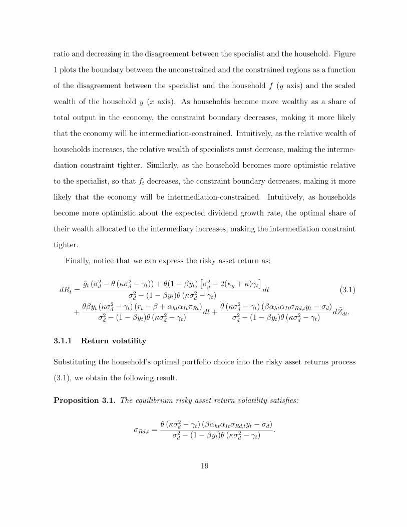
of the realized dividend growth process to learn about gt. In addition, specialists can
observe an external, unbiased signal of the expected dividend growth rate of the form:
det = gtdt+σe√ntdZet, (2.4)
where σe > 0 is a constants, nt denotes the effort expanded by the specialist in acquiring
information and dZet is the increment of the standard Brownian motion, independent of
both dZdt and dZgt. I assume that the specialists face a capacity constraint in processing
the external signal, with the total information transmission rate to the specialist from
observations of both the realized dividend growth rate dDt/Dt and the external signal
bounded above by a constant. As in Sims (2003, 2006), this can be interpreted as a
physical constraint in processing information. The actual act of observing the external
signal is also costly to the specialist in a monetary sense, with the per-unit-of-wealth cost
of the effort required to observe an external signal of a given precision proportional to the
increase in the information transmission rate to the specialist. This second cost corre-
sponds to the cost of information production (data collection and noise reduction). Both
of these frictions prevent the specialist from “growing out” of the information constraint
as his wealth increases. For a more detailed discussion of the different specifications of
the information acquisition trade off, see Boyarchenko and Duarte (2012).
Given the strategic choice to acquire information, it is not immediate that standard
filtering results apply. Detemple and Kihlstrom (1987), however, show that, even with
strategic information choice, the specialist’s beliefs are given by the Kalman-Bucy filter.
In particular:
Lemma 2.1. (Kalman-Bucy Filter)
Given the time t information set Ft = σ− {Ds, es : s ≤ t}, the specialist’s inference at
8

time t of the expected dividend growth rate has a Gaussian distribution: gt|Ft ∼ N (gt, γt),
with the inferred growth rate gt evolving according to:
dgt = κg (g − gt) dt+γtσddZdt +
γt√nt
σedZet, (2.5)
and the conditional variance of the belief as:
dγtdt
= −2κgγt + σ2g − γ2t
(1
σ2d
+ntσ2e
). (2.6)
Here, dZdt and dZet are independent increments of the standard Brownian motion under
Ft, given, respectively, by:
dZdt = σ−1d
(dDt
Dt
− gtdt)
dZet =
√ntσe
(det − gtdt) .
Proof. See e.g. Theorem 10.2 of Liptser and Shiryaev (1977).
Notice also that, under the specialist’s information set Ft, the signal vector evolves as:
dD
D= gtdt+ σddZdt
det = gtdt+σe√ntdZet.
Recall that the household learns about the expected dividend growth rate g using
observations of the realized dividend growth rate only. Denote by Fht = σ− {Ds : s ≤ t}
the household’s information set at time t. Similarly to the belief evolution of the specialist,
the household’s inference at time t of the expected dividend growth rate has a Gaussian
distribution: gt|Fht ∼ N(ght, γht), with the inferred dividend growth rate ght evolving
9

according to:
dght = κg (g − ght) +γhtσddZh
dt,
and the conditional variance of the belief as:
dγhtdt
= −2κgγht + σ2g −
γ2htσ2d
,
where dZhdt is the increment of the standard Brownian motion under Fht , given by:
dZhdt = σ−1d
(dDt
Dt
− ghtdt).
Given the Gaussian structure of the observations-state system, the information trans-
mission rate to the specialist is given by:
dIdt
(g;Dt, et) =1
2E[
(gt − gt)2(
1
σ2d
+ntσ2e
)∣∣∣∣Ft]=γt2
(1
σ2d
+ntσ2e
). (2.7)
For a proof of the above result, see e.g. Turmuhambetova (2005). Compare this to the
information transmission rate to the household:
dIh
dt(g;Dt) =
γht2σ2
d
.
While the specialist and the household are both relatively uninformed, so that γht and
γt are of similar magnitude, the information transmission rate to the specialist is higher
since the specialist observes an additional signal. When the specialist becomes relatively
10

more informed, so that γht is much higher than γt, the information transmission rate to
the household as higher. Intuitively, for the less informed agent, every new observation
contains more new information than for the more informed agent.
I assume that the information transmission rate to the specialist is bounded above by
a constant κ > 0:
dIdt
(g;Dt, et) ≤ κ ∀t ≥ 0,
and that the cost of observing an external signal of precision√nt/σe is proportional to
the implied increase in the information transmission rate to the specialist:
wtθγtntσ2e
dt.
The parameter θ, which measures the marginal cost of increasing signal precision, per
unit of wealth×variance, can be interpreted as the aversion of the specialist to exerting
effort to observe additional signals of the long-term component of dividend growth rates.
In the appendix, I show that the value function of the specialist is strictly increasing the
precision of the external signal, so that he always chooses the signal precision to just
satisfy the capacity constraint. Thus, the per-period cost of the external signal can be
expressed as:
wtθ
(2κ− γt
σ2d
)dt.
Introduce ft = gt−ght to be the disagreement between the specialist and the household
about the expected dividend growth rate. Under the specialist’s information set Ft,
11

disagreement evolves as:
dft = −(κg +
γhtσ2d
)ftdt+
(γt − γhtσd
)dZdt +
γt√nt
σedZet.
Thus, disagreement follows a mean-reverting process, with variation in the speed of mean-
reversion determined by the information transmission rate to the household. Notice also
that, when the household is more uncertain about its inference of the expected dividend
growth rate, so that γht is large, disagreement is negative correlated with the innovations
to the dividend growth process.
Finally, we can parametrize the evolution of the risky asset return under the specialist’s
information set Ft as:
dRt = µRtdt+ σRd,tdZdt + σRe,tdZet,
and under the household’s information set Fht as:
dRt = µhRtdt+ σhRd,tdZhdt.
Since the specialist and the household agree about the risky asset price in equilibrium,
we can also represent the risky asset return under the specialist’s information set as:
dRt =
(µhRt +
σRd,tσd
ft
)dt+ σhRd,tdZdt.
12

Equating coefficients, we see that, in equilibrium:
σhRd,t = σRd,t
σRe,t = 0
µhRt = µRt −σRd,tσd
ft.
Thus, even though the innovations in the external signal inform the specialist’s beliefs,
they do not directly enter into the risky asset returns process. Notice also that, when
the household is more optimistic than the specialist about the expected dividend growth
rate, so that ft < 0, the household believes the expected risky asset return to be higher as
well. In the following, I denote by πRt = µRt − rt the risk premium under the specialist’s
information set; under the household’s information set, the risk premium is given by
πRt − σRd,tft/σd.
2.3 State variables
It is useful at this point to summarize the state variables in the economy and their
evolutions under the specialist’s information set. Since the specialist is the marginal
investor in both the risky and the risk-free asset markets, asset prices satisfy his Euler
equation and, hence, the specialist’s information set is the relevant one in determining
the time series behavior of returns. The full state vector in the economy is:
(gt, ft, γt, γht, yt, wt, wht) .
Here, yt = wht/Dt is the relative wealth of the household. Since the households are
constrained in their portfolio allocation decision, their relative wealth will be a driving
13

factor for asset prices and, hence, the wealth evolutions in the economy. An alternative
specification would be to have the current dividend Dt as a state variable instead of yt;
however, this specification turns out to lead to more parsimonious asset pricing formulas.
Parametrize the evolution of yt under the specialist’s information set as:
dyt = µytdt+ σyd,tZdt.
Notice that, since innovations to the external signal do not affect the evolution of the risky
asset return, they will not affect the evolution of the relative wealth of the household.
Notice also that, in an economy with households only, yt corresponds to the inverse of the
consumption-wealth ratio cayt of Lettau and Ludvigson (2001), which has been shown to
predict stock returns.
2.4 Specialist’s problem
Since specialists are the only agents with access to the risky asset market, I assume that
the specialists makes all of the investment decisions on the total capital of the intermediary
and faces no portfolio restrictions in buying or short-selling either the risky asset or the
risk-free bond. In particular, denote by αIt the fraction of intermediary capital invested
in the risky asset at time t and by wt the specialist wealth at time t. Notice that, since
all of the specialist’s wealth is invested in the intermediary, αIt is the effective exposure
of the specialist to the risky asset. Then:
Proposition 2.2. The specialist chooses his consumption rate, his information acquisition
and the intermediary’s exposure to the risky asset to solve:
max{ct,αIt,nt}
E[∫ +∞
0
e−βt log ctdt
], (2.8)
14

subject to the specialist’s budget constraint:
dwt = −ctdt+ wtrtdt+ αItwt (dRt − rtdt)− wtθ(
2κ− γtσ2d
)dt.
The specialist’s optimal consumption rule is:
ct = βwt, (2.9)
the optimal risk exposure is:
αIt =πRtσ2Rd,t
, (2.10)
and the optimal external signal precision is:
nt =
(2κ
γt− 1
σ2d
)σ2e . (2.11)
Thus, the specialist consumes a fixed proportion, β, of his wealth each period, and invests
according to the standard myopic investment rule. The optimal signal precision increases
with the precision of the specialist’s beliefs. Intuitively, as the beliefs of the specialist
become more precise, the same rate of information transmission is attained with a higher
signal precision.
2.5 Household’s problem
Consider now the household’s problem. Denote by αht ∈ [0, 1] the fraction of household
wealth allocated to the intermediary at time t. As in He and Krishnamurthy (2010),
I assume that the household is precluded from shorting both the intermediary and the
15

risk-free bond. Then the following result holds.
Proposition 2.3. Taking the specialist’s wealth wt and exposure choice αIt as given, the
household solves:
max{cht,αht}
E[∫ +∞
0
e−βt log chtdt
], (2.12)
subject to the household’s budget constraint:
dwht = −chtdt+ whtrtdt+ αhtαItwht (dRt − rtdt) ,
the intermediation constraint:
αhtwht ≤ mwt,
and the no shorting constraint: αht ∈ [0, 1]. The household’s optimal consumption rule is:
cht = βwht, (2.13)
and the optimal risk exposure in the unconstrained region is:
αht =πRt − σRd,tσ−1d ft
αItσ2Rd,t
. (2.14)
Thus, in the unconstrained region, the household also acts as a standard myopic investor,
consuming a constant proportion of its wealth each period.
16

2.6 Equilibrium
Definition 2.4. An equilibrium in this economy is a set of price processes {Pt} and {rt},
and decisions {ct, cht, αIt, αht, nt} such that:
1. Given the price processes, decisions solve the consumption-savings problems of the
specialist (2.8) and the household (2.12).
2. Decisions satisfy the intermediation constraint.
3. The risky asset market clears:
αIt (wt + αhtwht) = Pt. (2.15)
4. The goods market clears:
ct + cht = Dt. (2.16)
Notice that, since the risk-free bonds are in equilibrium zero-net supply, the risky asset
market clearing condition can be expressed as:
wt
(1− θ
(κ− γt
σ2d
))+ wht = Pt.
3 Asset prices
In this section, I characterize the asset prices in the economy. Notice that, since the
households are (potentially) constrained in making their investment decisions by the in-
termediation constraint, the specialist is the marginal agent in both the risky and the
17

risk-free asset markets. In particular, the risk-free rate in the economy satisfies the Euler
equation of the specialist but not necessarily that of the household.
3.1 Risky asset price
Begin by considering the risky asset price. Since the specialists and the households in this
economy have log preferences, we can derive the risky asset price in closed form. Substi-
tuting the specialist’s (2.9) and the household’s (2.13) optimal consumption decisions into
the goods market clearing condition (2.16), the price of the risky asset can be expressed
as:
Pt =Dt
βσ2d
[σ2d − θ
(κσ2
d − γt)]
+θ
σ2d
(κσ2
d − γt)wht.
Thus, the equilibrium price-dividend ratio is given by:
PtDt
=1
βσ2d
[σ2d − θ
(κσ2
d − γt)]
+θ
σ2d
(κσ2
d − γt)yt.
Recall that the economy is intermediation-constrained when the specialist has rela-
tively low wealth, so that:
αht =πRt − σRd,tσ−1d ft
αItσ2Rd,t
>mwtwht
.
Rewriting, we obtain:
yt ≥mπRt
β[(1 +m) πRt − σRd,tσ−1d ft
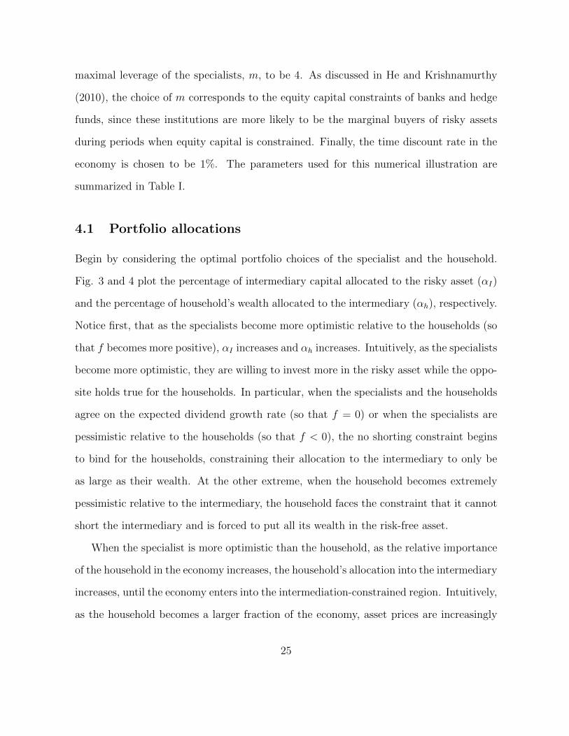
] .Thus, the y boundary of the intermediation-constrained region is increasing in the Sharpe
18
ratio and decreasing in the disagreement between the specialist and the household. Figure
1 plots the boundary between the unconstrained and the constrained regions as a function
of the disagreement between the specialist and the household f (y axis) and the scaled
wealth of the household y (x axis). As households become more wealthy as a share of
total output in the economy, the constraint boundary decreases, making it more likely
that the economy will be intermediation-constrained. Intuitively, as the relative wealth of
households increases, the relative wealth of specialists must decrease, making the interme-
diation constraint tighter. Similarly, as the household becomes more optimistic relative
to the specialist, so that ft decreases, the constraint boundary decreases, making it more
likely that the economy will be intermediation-constrained. Intuitively, as households
become more optimistic about the expected dividend growth rate, the optimal share of
their wealth allocated to the intermediary increases, making the intermediation constraint
tighter.
Finally, notice that we can express the risky asset return as:
dRt =gt (σ2
d − θ (κσ2d − γt)) + θ(1− βyt)
[σ2g − 2(κg + κ)γt
]σ2d − (1− βyt)θ (κσ2
d − γt)dt (3.1)
+θβyt (κσ2
d − γt) (rt − β + αhtαItπRt)
σ2d − (1− βyt)θ (κσ2
d − γt)dt+
θ (κσ2d − γt) (βαhtαItσRd,tyt − σd)
σ2d − (1− βyt)θ (κσ2
d − γt)dZdt.
3.1.1 Return volatility
Substituting the household’s optimal portfolio choice into the risky asset returns process
(3.1), we obtain the following result.
Proposition 3.1. The equilibrium risky asset return volatility satisfies:
σRd,t =θ (κσ2
d − γt) (βαhtαItσRd,tyt − σd)σ2d − (1− βyt)θ (κσ2
d − γt).
19

Thus, in the intermediation-unconstrained region, the risky asset return volatility is given
by:
σRd,t = − θ (κσ2d − γt)σd
σ2d − (1− βyt)θ (κσ2
d − γt)+
θ (κσ2d − γt) βyt
σ2d − (1− βyt)θ (κσ2
d − γt)
(πRtσRd,t
− ftσd
).
When the economy is in the intermediation-constrained region, the risky asset return
volatility becomes:
σRd,t = − θ (κσ2d − γt)σd
σ2d − (1− βyt)θ (κσ2
d − γt)+
θ (κσ2d − γt) (1− βyt)
σ2d − (1− βyt)θ (κσ2
d − γt)πRtσRd,t
.
Notice that, in the intermediation-constrained region, the risky asset return volatil-
ity does not depend on the disagreement between the specialist and the household while
the disagreement does influence the volatility in the unconstrained region. Intuitively, in
the intermediation-constrained region, the households are constrained in choosing their
portfolio allocation, and are thus the inframarginal investors in the risky asset. Thus,
the price of the risky asset in the constrained region reflects only the beliefs of the spe-
cialist. In the unconstrained region, both the specialist and the household are at their
unconstrained optimum, so the risky asset price balances both of their beliefs. Notice also
that, unlike the perfect information setting of He and Krishnamurthy (2011), the disagree-
ment between the specialist and the household and the learning process of the specialist
introduce stochastic volatility in the returns process even in the unconstrained region.
The volatility of the returns process is increasing in the Sharpe ratio of the risky asset,
both in the constrained and the unconstrained region of the economy. Notice also that,
asymptotically, as yt → +∞, which corresponds to the economy becoming increasingly
more intermediation-constrained, σ2Rd,t → −πRt. Intuitively, as the household becomes
infinitely large relative to the economy, asset prices converge to the shadow asset prices in
20

an economy where the household is the only agent in the economy, but cannot trade in the
risky asset. At the other extreme, as yt → 0, so that the economy becomes increasingly
less intermediation-constrained,
limyt→0
σRd,t =θ (κσ2
d − γt)σdθ (κσ2
d − γt)− σ2d
.
Thus, as the specialist becomes the dominant agent in the economy, the risky asset volatil-
ity depends only on the fluctuation in the beliefs of the specialist. In particular, in the
long-run equilibrium of the information acquisition (with γt =σ2g
2(κ+κg)), the risky asset
volatility will be constant.
3.1.2 Risk premium
We can also use the risky asset returns process (3.1) to obtain the equilibrium risk pre-
mium.
Proposition 3.2. The equilibrium risk premium satisfies:
πRt = −β +θ[σ2g − 2 (κg + κ) γt
](1− βyt)
σ2d − (1− βyt)θ (κσ2
d − γt)+
(σd − βytαhtαItσRd,t)2
(1− βyt)2
+βytσ
2d [rt − β − gt + αhtαItπRt]
(1− βyt) (σ2d − (1− βyt)θ (κσ2
d − γt)).
Thus, in the intermediation-unconstrained region, the risk premium is given by:
πRt = −β +θ[σ2g − 2 (κg + κ) γt
](1− βyt)
σ2d − (1− βyt)θ (κσ2
d − γt)+
βytσ2d [rt − β − gt]
(1− βyt) (σ2d − (1− βyt)θ (κσ2
d − γt))
+βytσ
2d
(1− βyt) (σ2d − (1− βyt)θ (κσ2
d − γt))
(πRtσRd,t
− ftσd
)πRtσRd,t
+
(σd
1− βyt− βyt
1− βyt
(πRtσRd,t
− ftσd
))2
.
21

When the economy is in the intermediation-constrained region, the risk premium becomes:
πRt = −β +θ[σ2g − 2 (κg + κ) γt
](1− βyt)
σ2d − (1− βyt)θ (κσ2
d − γt)+
βytσ2d [rt − β − gt]
(1− βyt) (σ2d − (1− βyt)θ (κσ2
d − γt))
+mσ2
d
(σ2d − (1− βyt)θ (κσ2
d − γt))π2Rt
σ2Rd,t
+
(σd
1− βyt−m πRt
σRd,t
)2
.
Similarly to the risky asset return volatility, in the intermediation-constrained region,
the risk premium does not depend on the disagreement between the specialist and the
household while the disagreement does influence the risk premium in the unconstrained
region. Asymptotically, as yt → +∞, the risk premium becomes:
limyt→+∞
πRt = − β
1 +m2− 1
1 +m2
[σ2g − 2 (κg + κ) γt
](κσ2
d − γt)− [rt − β − gt] .
In the long-run equilibrium of the information acquisition, this becomes
πRt → −β
1 +m2− [rt − β − gt] .
At the other extreme, as yt → 0, the equilibrium risk premium converges to:
limyt→0
πRt = −β +θ[σ2g − 2 (κg + κ) γt
]σ2d − θ (κσ2
d − γt)+ σ2
d.
As with the risky asset return volatility, as the specialist becomes the dominant agent in
the economy, the equilibrium risk premium is determined by fluctuations in his beliefs.
In the long-run equilibrium of the information acquisition, the risk premium becomes
πRt → σ2d − β.
22

3.2 Risk-free rate
Since the specialist is the marginal investor in the risk-free market, the risk-free rate
satisfies the specialist’s Euler equation:
rtdt = βdt+ E[dwtwt
∣∣∣∣Ft]− var( dwtwt
∣∣∣∣Ft) .Notice that we can represent:
dwtwt
=d (Dt − βwht)Dt − βwht
=dDt/Dt − βdwht/Dt
1− βyt
This yields the following result.
Proposition 3.3. The equilibrium risk-free rate is given by:
rt − β − gt = −βytαhtαItπRt −(σd − βytαhtαItσRd,t)2
1− βyt.
Thus, in the intermediation-unconstrained region, the risk-free rate is given by:
rt − β − gt = −βyt(πRtσRd,t
− ftσd
)πRtσRd,t
− 1
1− βyt
(σd − βyt
(πRtσRd,t
− ftσd
))2
.
When the economy is in the intermediation-constrained region, the risk-free rate becomes:
rt − β − gt = −m(1− βyt)π2Rt
σ2Rd,t
− 1
1− βyt
(σd −m
πRtσRd,t
(1− βyt))2
.
Thus, the risk-free rate is increasing in the expected long-run dividend growth rate
and decreasing in the Sharpe ratio in both the constrained and the unconstrained regions
23

of the economy. Asymptotically, as yt → +∞, the risk-free rate becomes:
limyt→+∞
rt = −∞.
Intuitively, as the household becomes the dominant agent in the economy, the demand
for borrowing by the specialist decreases, while the supply of credit by the households
increases, driving the equilibrium interest rate to −∞. At the other extreme, as yt → 0,
the equilibrium risk-free rate converges to:
limyt→0
rt = β + gt − σ2d.
Thus, as the specialist becomes the dominant agent in the economy, the risk-free rate is
determined by his beliefs about the long-run expected dividend growth rate.
4 Numerical Illustration
In this section, I examine the behavior of the equilibrium asset prices and portfolio allo-
cation choices for some calibrated parameters. For the parameters of the dividend growth
process, the long-run mean of the dividend growth process, and the external signal, I
adapt the calibration of Bansal and Yaron (2004) for my specification. The capacity of
the specialist to process information, κ, is chosen to make the initial information choice
0:
κ =1
2
γ0σ2d
,
and the prior variance of the specialist’s (γ0) and the household’s (γh0) belief are chosen
to be 1. I explore the impact of varying the marginal cost of observing better information,
θ, on the equilibrium asset prices. As in He and Krishnamurthy (2010, 2011), I choose the
24
maximal leverage of the specialists, m, to be 4. As discussed in He and Krishnamurthy
(2010), the choice of m corresponds to the equity capital constraints of banks and hedge
funds, since these institutions are more likely to be the marginal buyers of risky assets
during periods when equity capital is constrained. Finally, the time discount rate in the
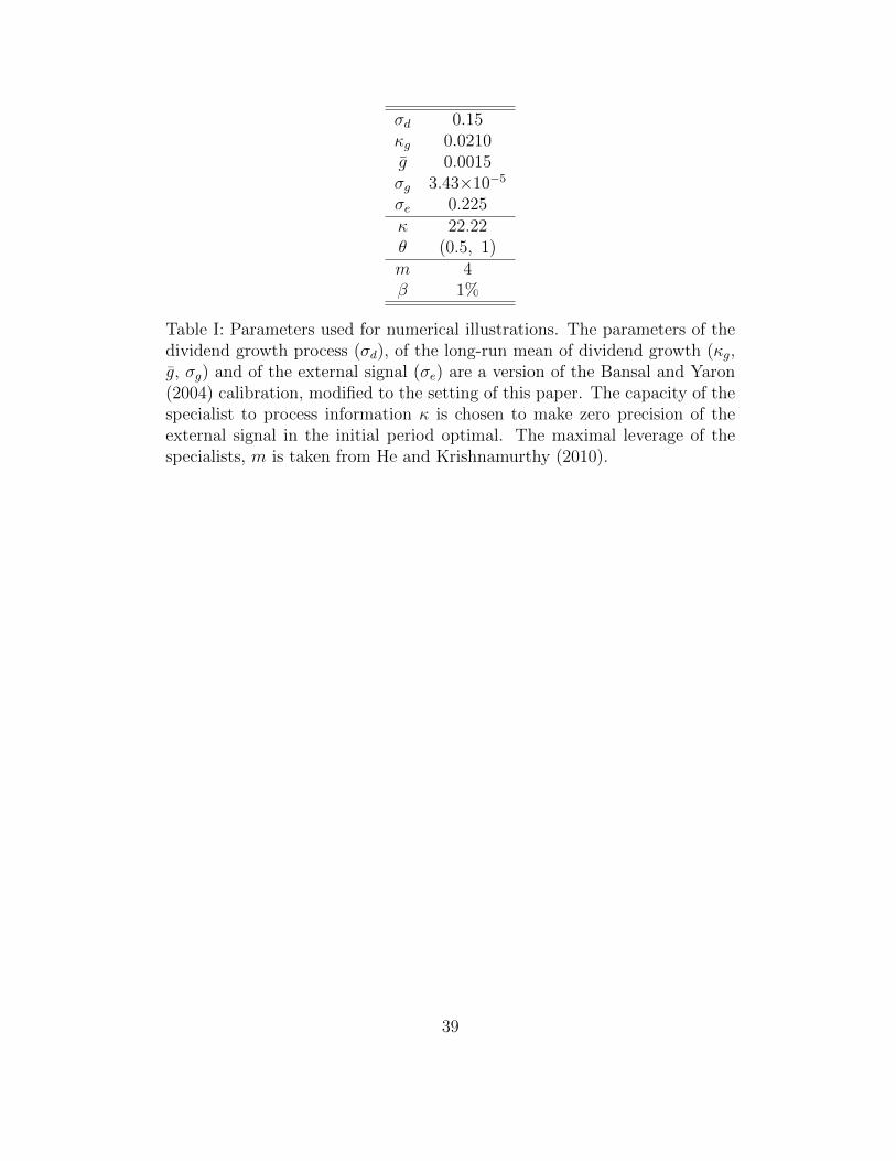
economy is chosen to be 1%. The parameters used for this numerical illustration are
summarized in Table I.
4.1 Portfolio allocations
Begin by considering the optimal portfolio choices of the specialist and the household.
Fig. 3 and 4 plot the percentage of intermediary capital allocated to the risky asset (αI)
and the percentage of household’s wealth allocated to the intermediary (αh), respectively.
Notice first, that as the specialists become more optimistic relative to the households (so
that f becomes more positive), αI increases and αh increases. Intuitively, as the specialists
become more optimistic, they are willing to invest more in the risky asset while the oppo-
site holds true for the households. In particular, when the specialists and the households
agree on the expected dividend growth rate (so that f = 0) or when the specialists are
pessimistic relative to the households (so that f < 0), the no shorting constraint begins
to bind for the households, constraining their allocation to the intermediary to only be
as large as their wealth. At the other extreme, when the household becomes extremely
pessimistic relative to the intermediary, the household faces the constraint that it cannot
short the intermediary and is forced to put all its wealth in the risk-free asset.
When the specialist is more optimistic than the household, as the relative importance
of the household in the economy increases, the household’s allocation into the intermediary
increases, until the economy enters into the intermediation-constrained region. Intuitively,
as the household becomes a larger fraction of the economy, asset prices are increasingly
25
more reflective of the household’s belief, in addition to that of the specialist, making
households more likely to invest in the risky asset. This effect also accounts for the
opposite behavior of the specialist’s portfolio choice: for large optimism on the part of the
specialist, the fraction of intermediary capital allocated to the intermediary increases as
the scaled wealth of the household increases while the household is constrained to invest
0, but decreases when the household is finally able to enter the market. When the beliefs
of the specialist and the household are more in sync, the fraction of intermediary capital
allocated to the risky asset increases for some range out the household’s scaled wealth in
the region where the household is not constrained, but decreases for larger values of y.
Notice that, while the marginal cost of information acquisition θ only has a small
effect on the peak of intermediary investment in the risky asset, the cost does have a
large effect on the degree of divestment when the intermediation constraint binds. In
particular, for the case of low cost of information acquisition, the specialists divest more
aggressively, driving up risk premia. This is similar to the hold-up problem encountered in
the contracting literature1: when the cost of acquiring information about an asset is high,
the specialist is willing to hold on to the asset longer to recuperate the costs associated
with the investment in information.
Notice finally that either when the household is constrained to invest 0 is the in-
termediary (low values of y, high values of f) or when the household is constrained to
invest 1 is the intermediary (low values of y, low values of f) or when the economy is
in the intermediation-constrained region (high values of y, low values of f), the portfolio
allocation choice does not depend on the disagreement between the specialist and the
household.2 Intuitively, because of one constraint or the other, the household is precluded
1See e.g. Klein et al. (1978); Williamson (1979, 1985); Grossman and Hart (1986); Hart and Moore(1990)
2See Fig. 2 for a graphical illustration of the four regions of the economy.
26
from participating effectively in the risky asset market and, thus, the difference between
beliefs does not play a role. Disagreement does however determine for which relative sizes
of the household sector the economy enters one of the constrained sectors.
4.2 Asset prices
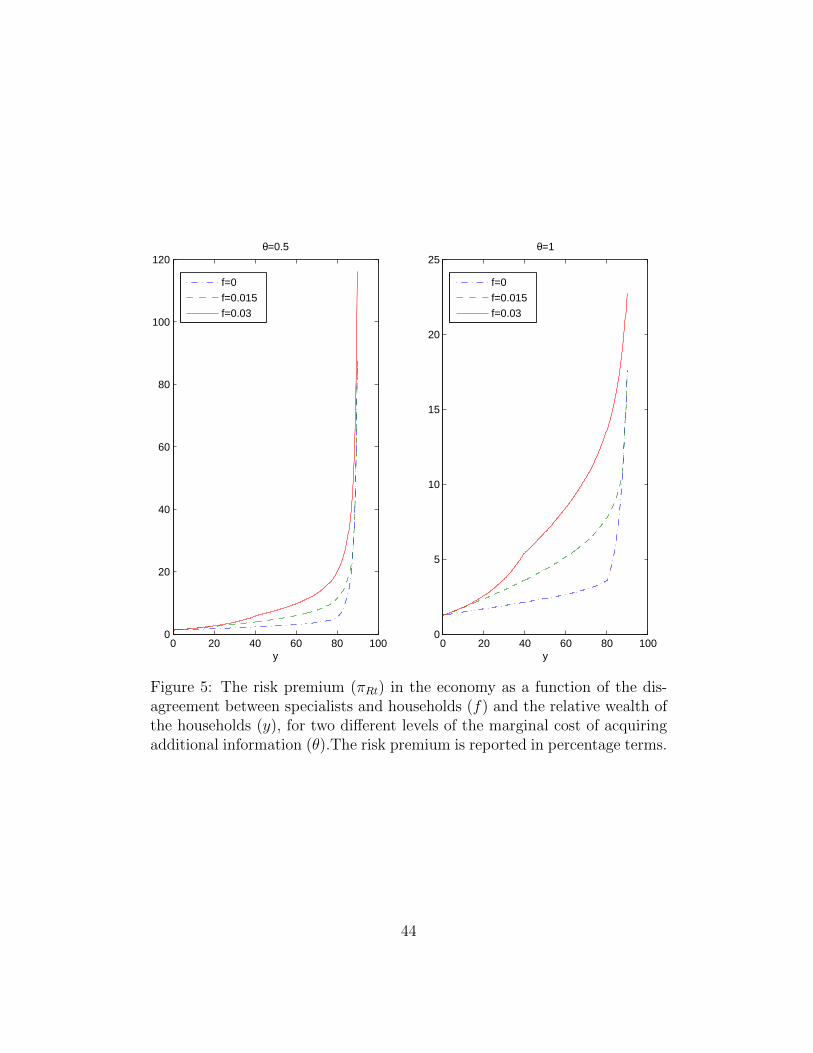
Consider next risk premium in the economy (Fig. 5). Since the specialists are the agents
that hold the risky assets in this economy, it is not surprising that the risk premium in
the economy increases as the specialists become more optimistic. Further, as the relative
wealth of the household increases, the risky asset is distributed across a smaller mass of
specialists, increasing the required risk premium. This effect becomes more pronounced
in the intermediation-constrained region, since the specialists cannot fully supplement
their own funds with household contributions in clearing the risky asset market, driving
the risk premium up. Notice also that, while the effect of changing the marginal cost of
information (θ) was small for the optimal portfolio allocations, higher costs of processing
information reduces the risk premium. Intuitively, since the information acquisition costs
are paid by the specialist, increasing the cost of information is equivalent to increasing
the long-run equilibrium time-discount rate of the specialist, lowering the risk premium
that specialists are willing to pay for holding the risky asset.
The risky asset volatility (Fig. 6) mimics the behavior of the risk premium: as the
specialists become more optimistic relative to the households or as the scaled household
wealth becomes larger, the risky asset volatility increases. Intuitively, since disagreement
is mean-reverting around zero, as the specialists become more optimistic, the probability
of disagreement declining increases, increasing the volatility. As the household becomes
more dominant in the economy, the risky asset is distributed among a smaller mass of
specialists, so shocks to the dividend growth rate become amplified. Notice, however,
27

that the increases in the risk premium are not perfectly off-set by the increase in the
risky asset volatility: the Sharpe ratio of the risky asset (Fig. 7) is also increasing in the
disagreement between the specialist and the household and in the scaled wealth of the
household.
Consider finally the risk-free rate in the economy (Fig. 8). As the specialist becomes
more optimistic relative to the household, the risk-free rate decreases. Intuitively, as the
specialist becomes more optimistic, the household is less willing to invest in the risky asset
and, hence, more willing to invest in the risk-free asset, lowering the interest rate. The
risk-free rate also decreases as the household becomes more dominant in the economy.
Thus, as the scaled household wealth increases, the lending demand by specialists is
distributed across a larger mass of households, lowering the risk-free rate. Notice that
this is the risk-free asset market counterpart to the mechanism that increases the risk
premium (and the Sharpe ratio) as specialists become less dominant in the economy.
Since the asset markets must clear in equilibrium, the relative size of the natural owners
of the two types of assets (households for the risk-free asset and specialists for the risky
asset) impacts the level of the expected return in the corresponding markets.
Notice finally that, as with optimal portfolio choice, asset prices do not depend on
the disagreement between the specialist and the household when either the household
is constrained to invest 0 is the intermediary (low values of y, high values of f) or the
household is constrained to invest 1 is the intermediary (low values of y, low values of f)
or the economy is in the intermediation-constrained region (high values of y, low values
of f). Since the households are constrained in their portfolio choice in those regions, they
are infra-marginal investors and their beliefs do not impact asset prices.
28
5 Empirical Analysis
In this section, I conduct some simple exploratory empirical analysis to examine testable
predictions of the model. First, during “normal” times, stock volatility should be directly
impacted by the disagreement between the households and the specialists, whereas the in-
dividual beliefs of the households only enter indirectly through an impact on risk premia.
Second, during periods when the specialists are liquidity constrained, household beliefs
should have a direct impact on volatility. Finally, the beliefs of both specialists and house-
holds should command a risk premium during normal times, with the risk premium on
household beliefs increasing during period when specialists are liquidity constrained. The
empirical evidence is consistent with these predictions, although the degree of statistical
significance varies across specifications.
5.1 Data
In the empirical analysis, I interpret the disagreement between specialists and households
broadly and focus on variation in the pessimism about the overall future prospects of
the economy. As a proxy for the beliefs of the households, I use the Michigan Survey
of Consumer Expectations. Each month, 500 individuals are randomly selected from
the contiguous United States (48 states plus the District of Columbia) to participate in
the Surveys of Consumers. The questions asked cover three broad areas of consumer
confidence: personal finances, business conditions, and future buying plans, with the
respondents being asked to provide an assessment of both the current conditions and their
future expectations. The index is then constructed as follows: the number of negative
responses to each question is subtracted from the number of positive responses to the
question. The three resulting numbers are then averaged, with the index ranging between
29

-100 and +100.
I use the “anxious” index produced by the Federal Reserve Bank of Philadelphia as
a proxy for specialist beliefs. The anxious index measures the probability of a decline in
real GDP, as reported in the Survey of Professional Forecasters. The survey asks panelists
to estimate the probability that real GDP will decline in the quarter in which the survey
is taken and in each of the following four quarters. The anxious index is the probability
of a decline in real GDP in the quarter after a survey is taken. For example, in the survey
taken in the first quarter of 2012, the anxious index is 13.4 percent, which means that
forecasters believe there is a 13.4 percent chance that real GDP will decline in the second
quarter of 2012.
To make the two measures of beliefs compatible, I scale them to have zero mean and
unit variance. Further, since an increase in the Consumer Expectations Index implies
an improvement in households’ outlook, I reverse the sign of the Index before scaling.
The measure of disagreement is then constructed as the difference between the scaled
Consumer Expectations and the scaled Anxious Index.
Monthly observations of the two indexes are plotted in Fig. 9. As has been docu-
mented in the literature, both the Anxious Index and the Consumer Expectations Survey
are leading indicators of the business cycle, with the two measures increasing during reces-
sions. While both measures exhibit counter-cyclical behavior, they do no covary perfectly,
as can be seen from the resulting measure of disagreement in Fig. 10. Disagreement be-
tween the specialists and the households increases during booms, and decreases during
recessions.
30

5.2 Stock market volatility
According to the model, during normal times, an increase in the pessimism of households
relative to the specialists should lead to an increase in stock market volatility as households
start to exit the intermediation relation. To assess the significance of this association, I
consider the following regression:
V Ct = a+ bft + cV Ct−1 + et.
Here, V Ct is the realized stock market volatility, computed using daily returns of the S& P
500 index within the given quarter. Adding the lagged observations of volatility removes
most of the serial correlation in V C. I compute Newey-West standard errors with three
lags, and verify that using six lags leads to identical conclusions.
Table II reports the OLS estimates of the coefficients of interest and their t-statistics.
As the model predicts, an increase in the pessimism of households relative to the specialists
leads to more volatility, with the coefficient b > 0 on the measure of disagreement. The
coefficient is statistically significant in all three specifications, suggesting that stocks are
indeed more volatile when specialists are more pessimistic than households.
The model also predicts that households beliefs per se should not impact volatility
strongly during normal times (they do so only through an indirect impact on the risk
premium) but, during periods when the specialists are liquidity-constrained, increased
household pessimism should increase volatility. The last two regressions test this specifi-
cation:
V Ct = a+ bft + cV Ct−1 + dght + et
V Ct = a+ bft + cV Ct−1 + dght + hght1Recession + et.
31

While the signs of the coefficient on household pessimism and on the interaction term
between household pessimism and an NBER recession dummy are positive as predicted
by the model, the coefficient on household beliefs is only marginally statistically significant
and the interaction term coefficient is not statistically significant.
5.3 Equity risk premium
The model predicts that, during normal times, specialists’ optimism and the relative
pessimism of increase the risk premium paid on risky assets. To asset the significance of
this association, I consider the following regression:
Rt+1 = a+ bgt + cft + et.
Here, Rt+1 is the cumulative return on the CRSP value-weighted market portfolio over
the quarter following the date of the survey. As before, I compute Newey-West standard
errors with three lags.
Table III reports the coefficients of interest and their t statistics. Although the signs of
the estimated coefficients on specialists’ optimism and the disagreement between house-
holds and specialist coincide with the model-predicted ones, they are statistically insignif-
icant. There might be no unconditional risk premium associated with these measures of
specialists’ beliefs and the disagreement between households and specialists. It is also
possible, though, that 44 years of quarterly data is not enough to ensure sufficient power
for this test.
The model also predicts, that conditional on the specialists being liquidity constrained,
disagreement commands a smaller risk premium. The following regression tests that hy-
pothesis by introducing an interaction term between disagreement and an NBER recession
32

dummy:
Rt+1 = a+ bgt + cft + dft1Recession + et.
While, as expected, the coefficient on the interaction term between disagreement and the
recession dummy is negative, it is also not statistically significant.
6 Conclusion
As information potentially available to (sophisticated) market participants increases, op-
timal information acquisition and the costs of acquiring and processing information have
a larger effect on asset prices. This paper considers the problem of information acquisi-
tion in an intermediated market, with the specialist given access to superior technology
of acquiring information. The disparity in the learning technologies of the specialist and
the household introduces endogenous disagreement between the specialist and the house-
hold, changing the shape of the intermediation-constrained region of the economy, and
increasing the frequency of periods of when the intermediation constraint binds. Rela-
tive optimism on the part of the specialist increases the risk premium, risky asset return
volatility and the Sharpe ratio of the risky asset, but decreases the fraction of household
wealth allocated to the intermediary sector. I find some empirical support for the model’s
key predictions.
In the long-run information equilibrium of the economy, costly information acquisition
makes the specialists less likely to decrease their risky asset holding when the intermedia-
tion constraint binds. Intuitively, as the cost of observing signals increases, the specialist
is willing to participate more in the risky asset market to recuperate the costs associated
with information acquisition. This in turns leads the risk premium, risky asset return
33

volatility and the Sharpe ratio of the risky asset to increase less dramatically in the
intermediation-constrained region, since the risky asset is distributed across a larger mass
of agents.
34
References
F. Allen and D. Gale. Limited market participation and volatility of asset prices. AmericanEconomic Review, 84:933–955, 1994.
R. Bansal and A. Yaron. Risks for the long-run: A potential resolution of asset pricingpuzzles. Journal of Finance, 59:1481–1509, 2004.
S. Basak and D. Cuoco. An equilibrium model with restricted stock market participation.Review of Financial Studies, 11:309–341, 1998.
N. Boyarchenko and F. Duarte. Investing in capacity: Long-run effects of rational inat-tention. Unpublished working paper, Federal Reserve Bank of New York, 2012.
M. Brunnermeier and Y. Sannikov. A macroeconomic model with a financial sector.Unpublished working paper, 2010.
J.B. Detemple and R.E. Kihlstrom. Acquisition d’information dans un modele intertem-porel en temps continu. L’Actualite Economique. Revue d’analyse economique, 63:118–137, 1987.
D. Diamond and P. Dybvig. Bank runs, deposit insurance and liquidity. Journal ofPolitical Economy, 93:401–419, 1983.
D. Diamond and R. Rajan. Liquidity shortages and banking crises. Journal of Finance,60:2177–2207, 2005.
S. Grossman and O. Hart. The costs and benefits of ownership: A theory of vertical andlateral integration. Journal of Political Economy, 94:691–719, 1986.
V. Haddad. Concentrated Ownership and Asset Prices. Unpublished working paper,University of Chicago, 2012.
O. Hart and J. Moore. Property rights and the nature of the firm. Journal of PoliticalEconomy, 98:1119–1158, 1990.
Z. He and A. Krishnamurthy. Intermediary asset pricing. Working paper, 2010.
Z. He and A. Krishnamurthy. A model of capital and crises. Review of Economic Studies,2011.
B. Holmstrom and J. Tirole. Financial intermediation, loanable funds and the real sector.Quarterly Journal of Economics, 112:663–691, 1997.
H. Hong, W. Torous, and R. Valkanov. Do industries lead stock markets? Journal ofFinancial Economics, 83:367–396, 2007.
35

L. Huang and H. Liu. Rational inattention and portfolio selection. Journal of Finance,LXII(4):1999–2040, 2007.
M. Kacperczyk, S. Van Nieuwerburgh, and L. Veldkamp. Attention allocation over thebusiness cycle: Evidence from the mutual fund industry. Unpublished working paper,2011.
B. Klein, R. Crawford, and A. Alchian. Vertical integration, appropriable rents, and thecompetitive contracting process. Journal of Law and Economics, 21:297–326, 1978.
M. Lettau and S. Ludvigson. Consumption, aggregate wealth and expected stock returns.Journal of Finance, 56:815–849, 2001.
R. S. Liptser and A. N. Shiryaev. Statistics of Random Processes: I,II. Springer-Verlag,New York, 1977.
R.E. Lucas. Asset prices in an exchange economy. Econometrica, 46:1429–1446, 1978.
G. Mankiw and S. Zeldes. The consumption of stockholders and non-stockholdes. Journalof Financial Economics, 29:97–112, 1991.
J. A. Scheinkman and W. Xiong. Overconfidence and speculative bubbles. Journal ofPolitical Economy, 111:1183–1220, 2003.
C. Sims. Implications of rational inattention. Journal of Monetary Economics, 50:665–690, 2003.
C. Sims. Rational inattention: Beyond the linear quadratic case. The American EconomicReview, 96(2):158–163, 2006.
G.A. Turmuhambetova. Decision Making in an Economy with Endogenous Information.PhD thesis, University of Chicago, Department of Economics, 2005.
S. Van Nieuwerburgh and L. Veldkamp. Information acquisition and under-diversification.Review of Economic Studies, 77(2):779–805, 2010.
A. Vissing-Jorgensen. Limited asset market participation and the elasticity of intertem-poral substitution. Journal of Political Economy, 110:825–853, 2002.
O. Williamson. Transaction-cost economics: The governance of contractual relations.Journal of Law and Economics, 22:233–261, 1979.
O. Williamson. The Economic Institutions of Capitalism. New York Free Press, 1985.
36

A Proofs
A.1 Proof of Proposition 2.2
Denote by J the value function of the specialist at time t:
J(wt, gt, γt, ft, γht, yt) = max{cs,αIs,ns}
E[∫ +∞
t
e−βs log csds
].
We will guess and verify that J has the form:
J(wt, gt, γt, ft, γht, yt) =1
βlogwt + Γ(gt, γt, ft, γht, yt),
where Γ is an unknown function to be determined. Then the HJB of the specialist is givenby:
logwt + βΓ = maxct,αIt,
√nt
log ct +1
βwt
(−ct + wtrt + αItwtπRt − wt
θ
2γtntσ2e
)− 1
2βα2Itσ
2Rd,t
+ Γgκg (g − gt) +1
2Γggγ
2t
(1
σ2d
+ntσ2e
)− Γf
(κg +
γhtσ2d
)ft
+1
2Γff
((γt − γhtσd
)2
+γ2t ntσ2e
)− Γγ
(2κgγt − σ2
g + γ2t
(1
σ2d
+ntσ2e
))− Γγh
(2κgγht − σ2
g +γ2htσ2d
)+ Γyµyt +
1
2Γyyσ
2yd,t
+ Γfg
((γt − γhtσd
)γtσd
+γ2t ntσ2e
)+ Γfyσyd,t
(γt − γhtσd
)+ Γgyσyd,t
γtσd
+ φ1tγtσent + φ2t
(κ− γt
2
(1
σ2d
+ntσ2e
)),
where φ1t ≥ 0 is the time t Lagrange multiplier on the no forgetting constraint nt ≥ 0and φ2t ≥ 0 is the time t Lagrange multiplier on the capacity constraint. Taking the firstorder conditions, we obtain:
[ct] : ct = βwt
[αIt] : αIt =πRtσ2Rd,t
[√nt] :
θ
β=
(1
2Γgg − Γγ +
1
2Γff + Γfg
)γt + φ1t −
φ2t
2.
37

Since the first order condition for nt does not depend on nt, the specialist always chooseshis attention allocation to be at the capacity constraint.
A.2 Proof of Proposition 2.3
Denote by Jh the value function of the household at time t:
Jh(wht, gt, γt, ft, γht, yt) = max{chs,αhs}
E[∫ +∞
t
e−βhs log chsds
].
Similarly to the specialist’s problem, guess that Jh has the form:
Jh(wht, gt, γt, ft, γht, yt) =1
βhlogwht + Γh(gt, γt, ght, γht, yt),
where Γh is an unknown function to be determined. Denote by λt/(βhwht) ≥ 0 the La-grange multiplier on the time t intermediation constraint, η1t ≥ 0 the Lagrange multiplieron the time t no intermediary shorting constraint of the household and by η2t the time tLagrange multiplier on the no risk-free bond shorting constraint. Then the HJB of thehousehold is given by:
wht + βhΓh = max
cht,αht
log cht +1
dtE[dΓh∣∣Fht ]
+1
βhwht
(−cht + whtrt + αhtαItwht(µ
hRt − rt)
)− 1
2βhα2htα
2It
(σhRd,t
)2+
λtβhwht
(mwt − αhtwht)− η1tαht + η2t (1− αht) .
Taking the first order conditions, we obtain:
[cht] : cht = ρhwht
[αht] : αht =µhRt − rt
αIt(σhRd,t
)2 − λt + η1t + η2t
α2It
(σhRd,t
)2 .
In the unconstrained region, λt = η1t = η2t = 0, so that (2.14) obtains.
38
σd 0.15κg 0.0210g 0.0015σg 3.43×10⁻⁵
σe 0.225κ 22.22θ (0.5, 1)m 4β 1%
Table I: Parameters used for numerical illustrations. The parameters of thedividend growth process (σd), of the long-run mean of dividend growth (κg,g, σg) and of the external signal (σe) are a version of the Bansal and Yaron(2004) calibration, modified to the setting of this paper. The capacity of thespecialist to process information κ is chosen to make zero precision of theexternal signal in the initial period optimal. The maximal leverage of thespecialists, m is taken from He and Krishnamurthy (2010).
39

y
f
θ=0.5
10 20 30 40 50 60 70 80−0.03
−0.02
−0.01
0
0.01
0.02
0.03
Figure 1: Intermediation-constrained and unconstrained regions of the econ-omy as a function of the disagreement between specialists and households(f) and the relative wealth of the households (y). The unconstrained regionis pictured in black and the constrained in white.
40

y
f
10 20 30 40 50 60 70 80−0.03
−0.02
−0.01
0
0.01
0.02
0.03
Figure 2: Intermediation-constrained (red), unconstrained (black), αht = 0(yellow) and αht = 1 (white) regions of the economy as a function of thedisagreement between specialists and households (f) and the relative wealthof the households (y).
41

0 20 40 60 80 1000
10
20
30
40
50
60
70
y
θ=0.5
f=0
f=0.015
f=0.03
0 20 40 60 80 10040
45
50
55
60
65
70
75
80
y
θ=1
f=0
f=0.015
f=0.03
Figure 3: The percent of intermediary capital allocated to the risky asset(αIt) in the economy as a function of the disagreement between specialistsand households (f) and the relative wealth of the households (y), for twodifferent levels of the marginal cost of acquiring additional information (θ).
42

0 20 40 60 80 1000
10
20
30
40
50
60
70
80
90
100
y
θ=0.5
f=0
f=0.015
f=0.03
0 20 40 60 80 1000
10
20
30
40
50
60
70
80
90
100
y
θ=1
f=0
f=0.015
f=0.03
Figure 4: The percent of household wealth allocated to the intermediary(αht) in the economy as a function of the disagreement between specialistsand households (f) and the relative wealth of the households (y), for twodifferent levels of the marginal cost of acquiring additional information (θ).
43
0 20 40 60 80 1000
20
40
60
80
100
120
y
θ=0.5
f=0
f=0.015
f=0.03
0 20 40 60 80 1000
5
10
15
20
25
y
θ=1
f=0
f=0.015
f=0.03
Figure 5: The risk premium (πRt) in the economy as a function of the dis-agreement between specialists and households (f) and the relative wealth ofthe households (y), for two different levels of the marginal cost of acquiringadditional information (θ).The risk premium is reported in percentage terms.
44

0 20 40 60 80 1000
50
100
150
200
250
300
350
400
y
θ=0.5
f=0
f=0.015
f=0.03
0 20 40 60 80 10010
20
30
40
50
60
70
80
y
θ=1
f=0
f=0.015
f=0.03
Figure 6: The risky asset volatility (σRt) in the economy as a function of thedisagreement between specialists and households (f) and the relative wealthof the households (y), for two different levels of the marginal cost of acquiringadditional information (θ).The risky asset volatility is reported in percentageterms.
45

0 20 40 60 80 1005
10
15
20
25
30
35
y
θ=0.5
f=0f=0.015f=0.03
0 20 40 60 80 1005
10
15
20
25
30
35
y
θ=1
f=0f=0.015f=0.03
Figure 7: The Sharpe ratio (πRt/σRt) in the economy as a function of thedisagreement between specialists and households (f) and the relative wealthof the households (y), for two different levels of the marginal cost of acquiringadditional information (θ).The Sharpe ratio is reported in percentage terms.
46

0 20 40 60 80 100−3
−2.5
−2
−1.5
−1
−0.5
0
0.5
y
θ=0.5
f=0
f=0.015
f=0.03
0 20 40 60 80 100−3
−2.5
−2
−1.5
−1
−0.5
0
0.5
y
θ=1
f=0
f=0.015
f=0.03
Figure 8: The risk-free rate (rt) in the economy as a function of the dis-agreement between specialists and households (f) and the relative wealth ofthe households (y), for two different levels of the marginal cost of acquiringadditional information (θ). The risk-free rate is reported in percentage terms.
47

−1
01
23
Anx
ious
Inde
x
−2
−1
01
2C
onsu
mer
Exp
ecta
tions
1968 1973 1978 1983 1988 1993 1998 2003 2008Date
Figure 9: The time series evolution of the Philadelphia Fed Anxious Index(left scale, solid line) and the Michigan Consumer Expectations Survey (rightscale, dashed line). Both time series have been scaled to have mean zeroand unit variance. NBER recessions are highlighted in grey. The MichiganConsumer Expectations Survey has been transformed so that an increase inthe level implies increased pessimism. Data source: Federal Reserve Bank ofPhiladelphia, Haver DLX.
48

−3
−2
−1
01
2D
isag
reem
ent
1968 1973 1978 1983 1988 1993 1998 2003 2008Date
Figure 10: The time series evolution of the disagreement between specialistsand households. Disagreement is measured as the difference between thePhiladelphia Fed Anxious Index and the Michigan Consumer ExpectationsSurvey, with the two components scaled to have mean zero and unit variance.NBER recessions are highlighted in grey. The Michigan Consumer Expec-tations Survey has been transformed so that an increase in the level impliesincreased pessimism. Data source: Federal Reserve Bank of Philadelphia,Haver DLX.
49
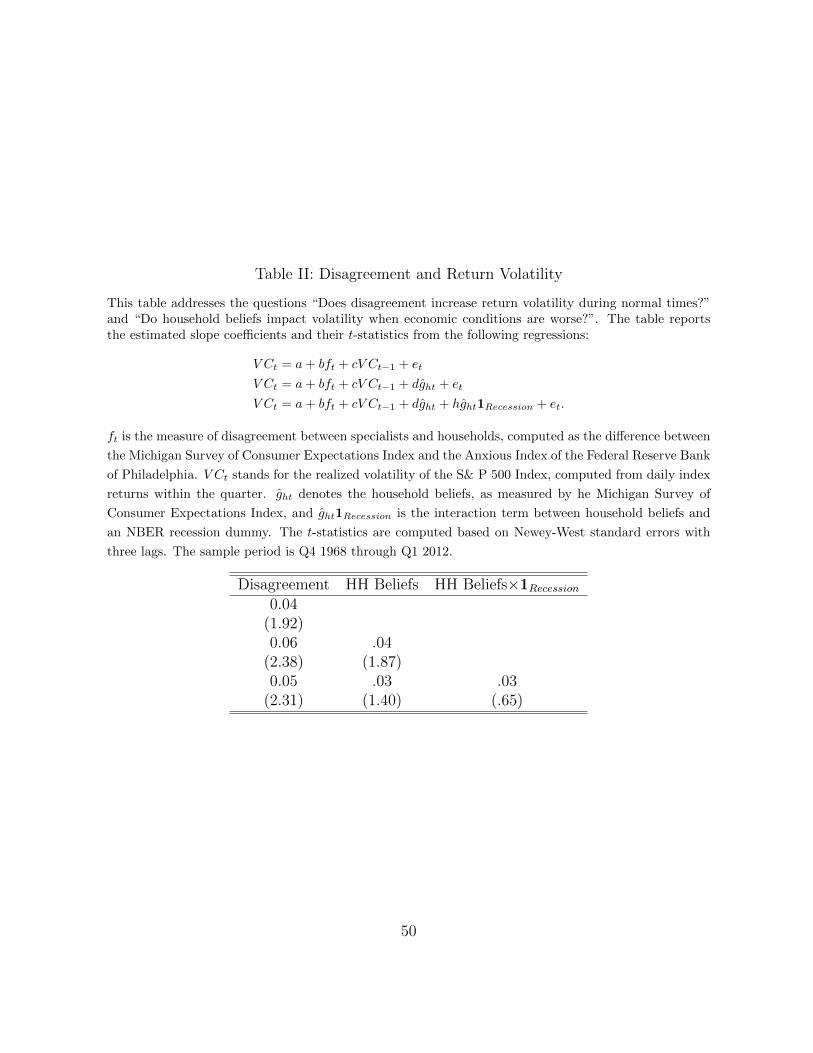
Table II: Disagreement and Return Volatility
This table addresses the questions “Does disagreement increase return volatility during normal times?”and “Do household beliefs impact volatility when economic conditions are worse?”. The table reportsthe estimated slope coefficients and their t-statistics from the following regressions:
V Ct = a + bft + cV Ct−1 + et
V Ct = a + bft + cV Ct−1 + dght + et
V Ct = a + bft + cV Ct−1 + dght + hght1Recession + et.
ft is the measure of disagreement between specialists and households, computed as the difference between
the Michigan Survey of Consumer Expectations Index and the Anxious Index of the Federal Reserve Bank
of Philadelphia. V Ct stands for the realized volatility of the S& P 500 Index, computed from daily index
returns within the quarter. ght denotes the household beliefs, as measured by he Michigan Survey of
Consumer Expectations Index, and ght1Recession is the interaction term between household beliefs and
an NBER recession dummy. The t-statistics are computed based on Newey-West standard errors with
three lags. The sample period is Q4 1968 through Q1 2012.
Disagreement HH Beliefs HH Beliefs×1Recession0.04
(1.92)0.06 .04
(2.38) (1.87)0.05 .03 .03
(2.31) (1.40) (.65)
50

Table III: Disagreement and Expected Returns
This table addresses the questions “Do specialist beliefs and disagreement between specialists and house-holds command a risk premium during normal times?” and “Does the risk premium on disagreementdecrease when economic conditions are worse?”. The table reports the estimated slope coefficients andtheir t-statistics from the following regressions:
Rt+1 = a + bgt + cft + et
Rt+1 = a + bgt + cft + dft1Recession + et.
Rt+1 is the aggregate stock market return in excess of the one month T-bill rate over the quarter fol-
lowing quarter t. ft is the measure of disagreement between specialists and households, computed as the
difference between the Michigan Survey of Consumer Expectations Index and the Anxious Index of the
Federal Reserve Bank of Philadelphia. gt stands for specialists’ beliefs, proxied for by the Anxious Index
of the Federal Reserve Bank of Philadelphia. ft1Recession is the interaction term between disagreement
and an NBER recession dummy. The t-statistics are computed based on Newey-West standard errors
with three lags. The sample period is Q4 1968 through Q1 2012.
Anxious Disagreement Disagreement×1Recession-0.25 .85
(-0.21) (.86)-0.25 0.85 -0.008
(-0.24) (0.82) (-0.003)
51


