Zum
Erlangen des akademischen Grades
DIPLOMINGENIEUR
(Dipl.-Ing.)
Betreuer: Dr.-Ing. Tino Schmiel, ILR TU-Dresden
Dipl. Wi.-Ing. Daniel Schubert, DLR Bremen
Verantwortlicher Hochschullehrer: Prof. Dr. Martin Tajmar, ILR TU-Dresden
Tag der Einreichung: 30.05.2012
Erster Gutachter: Prof. Dr. Martin Tajmar, ILR TU-Dresden
Zweiter Gutachter: Dipl. Wi.-Ing. Daniel Schubert, DLR Bremen
Diplomarbeit
ILR-RSN DA 12-03
System Analysis & Evaluation of Greenhouse
Modules within Moon/Mars Habitats
von
Paul Zabel

I
Selbstständigkeitserklärung (Declaration of Self-reliance)
Hiermit erkläre ich, dass ich die von mir dem Institut für Luft- und Raumfahrttechnik der Fa-
kultät Maschinenwesen der Technischen Universität Dresden eingereichte Studienarbeit
„Diplomarbeit“ zum Thema „System Analysis & Evaluation of Greenhouse Modules within
Moon/Mars Habitats“ selbstständig verfasst und keine anderen als die angegebenen Quellen
und Hilfsmittel benutzt sowie Zitate kenntlich gemacht habe.
_______________ ________________________
Ort, Datum Unterschrift des Studierenden
II
Abstract
Long term or even permanent settlement on different planets of the solar system is a fascina-
tion for mankind. Some researchers contemplate that planetary settlement is a necessity for
the survival of the human race over thousands of years. The generation of food for self-
sufficiency in space or on planetary bases is a vital part of this vision of space habitation. The
amount of mass that can be transported in deep space missions is constrained by the
launcher capability and its costs.
The space community has proposed and designed various greenhouse modules to cater to
human culinary requirements and act as part of life support systems. A survey of the different
greenhouse space concepts and terrestrial test facilities is presented, drawing a list of meas-
urable factors (e.g. growth area, power consumption, human activity index, etc.) for the eval-
uation of greenhouse modules. These factors include tangible and intangible parameters that
have been used in the development of an evaluation method on greenhouse concepts as a
subsystem of planetary habitats.
Überblick
Permanente Ansiedlungen auf anderen Planeten unseres Sonnensystems faszinieren die
Menschheit schon seit langem. Einige Forscher behaupten sogar, dass Siedlungen auf an-
deren Planeten für das Überleben der Menschheit über Tausende von Jahren notwendig
sind. Die Erzeugung von Nahrung im Weltraum oder in planetaren Habitaten ist für die
Selbstversorgung der Crew unverzichtbar und ein essentieller Bestandteil aller Visionen von
extraterrestrischen Kolonien. Ohne Selbstversorgung sind zukünftige Habitate auf Lieferun-
gen von der Erde angewiesen, die jedoch durch die Kapazität der Trägersysteme und die
entstehenden Kosten begrenzt sind.
Zahlreiche Entwürfe für Greenhouse-Module als Nahrungsquelle und Teil der Lebenserhal-
tungssysteme planetarer Habitate wurden bereits von Wissenschaftlern vorgeschlagen. In
der vorliegenden Arbeit wird eine Erfassung verschiedener Greenhouse-Konzepte und ter-
restrischer Testanlagen durchgeführt. Weiterhin erfolgt die Erstellung einer Liste messbarer
Vergleichsfaktoren (z.B. Anbaufläche, Energiebedarf). Die Faktoren beinhalten quantitative
und qualitative Parameter und werden für die Bewertung ausgesuchter Greenhouse-
Konzepte mit einer geeigneten Bewertungsmethode genutzt.
III
Table of Content
Selbstständigkeitserklärung (Declaration of Self-reliance) I
Abstract II
Table of Content III
List of Abbreviations VII
1 Introduction ........................................................................................................ 1
1.1 Motivation and Structure of Work 1
1.2 Previous Work 2
2 Scientific Background ....................................................................................... 3
2.1 Environmental Conditions 3
2.1.1 Free Space Environment 3
2.1.2 Local Environment of Moon and Mars 4
2.2 Human Requirements 6
2.3 Environmental Control and Life Support Systems 8
2.4 Survey on Past and Present Food Provision in Crewed Spacecraft 10
2.5 Greenhouse Module Subsystems 13
2.5.1 Classification 13
2.5.2 Fundamental & Interface Subsystems 13
2.5.3 Environmental Control Subsystems 14
2.5.4 Agricultural Subsystems 15
2.6 Summary 16
3 Development of an Analysis and Evaluation Strategy .................................. 17
3.1 Methodology 17
3.2 Analysis Method – The Morphological Analysis 18
3.3 Evaluation Methods 19
3.3.1 Equivalent System Mass 19
3.3.2 Analytical Hierarchy Process 22
3.4 Definition of Analysis and Evaluation Factors 27
3.4.1 Factor Categorization 27
3.4.2 Fundamental Factors 27
3.4.2.1 Definition 27
3.4.2.2 Module Shape 28
3.4.2.3 Arrangement of Growth Area 29

IV
3.4.2.4 Distribution of Aisles 31
3.4.2.5 Module Structure 33
3.4.2.6 Adaptability of Internal Configuration 34
3.4.2.7 Level of Automation 35
3.4.2.8 Module Mass, Dimensions and Volumes 35
3.4.2.9 Complexity 36
3.4.3 Environmental Factors 36
3.4.3.1 Definition 36
3.4.3.2 Lighting Type 37
3.4.3.3 Lighting Strategy 43
3.4.3.4 Atmospheric Composition 44
3.4.3.5 Trace Gas Treatment 45
3.4.3.6 Temperature Control 46
3.4.3.7 Photosynthetic Period 47
3.4.3.8 Humidity 48
3.4.3.9 Air Temperature 48
3.4.3.10 Atmospheric Pressure 49
3.4.3.11 Carbon Dioxide and Oxygen Partial Pressure 49
3.4.4 Agricultural Factors 49
3.4.4.1 Definition 49
3.4.4.2 Growth Medium 50
3.4.4.3 Plant Monitoring 52
3.4.4.4 Nutrient Supply 54
3.4.4.5 Plant Mixture 54
3.4.4.6 Planting Sequence 55
3.4.4.7 Cultivated Plants 56
3.4.4.8 Biomass Productivity 58
3.4.4.9 Specific Growth Area 58
3.4.4.10 Growth Height 59
3.4.5 Interface Factors 59
3.4.5.1 Definition 59
3.4.5.2 Water Purification 59
3.4.5.3 Air Revitalization 60

V
3.4.5.4 Resupply Dependency 61
3.4.5.5 Food Provision 62
3.4.5.6 Power Demand 62
3.4.5.7 Cooling Demand 62
3.4.5.8 Water In-/Output 62
3.4.5.9 Carbon Dioxide Input and Oxygen Output 62
3.4.5.10 Crew Size and Crew Work Load 63
3.4.5.11 Psychological Health Care 63
3.5 Summary 64
4 Demonstration of the Developed Evaluation Strategy .................................. 66
4.1 Description and Analysis of Selected Concepts and Testbeds 66
4.1.1 Survey on Existing Greenhouse Concepts 66
4.1.2 Lunar Greenhouse 73
4.1.3 Lunar Food and Revitalization Module 74
4.1.4 Biomass Production Chamber of BIO-Plex 76
4.2 Goal Definition for the Exemplary Evaluation 78
4.3 Establishing and Weighting of Evaluation Criteria 80
4.3.1 Selection of Evaluation Criteria 80
4.3.2 Calculation of Local and Global Weightings 82
4.4 Evaluation of Selected Concepts and Testbeds 85
4.5 Summary 87
5 Discussion ........................................................................................................ 88
6 Summary .......................................................................................................... 89
List of References X
Appendix 2-1: Recommended Macronutrient Daily Dietary Intake XVI
Appendix 2-2: Recommended Micronutrient Daily Dietary Intake XVII
Appendix 2-3: P/C Technologies for the Water Management XVIII
Appendix 2-4: P/C Technologies for Air Revitalization XIX
Appendix 3-1: Morphological Box of the LGH concept XX
Appendix 3-2: Morphological Box of the Lunar FARM concept XXI
Appendix 3-3: Morphological Box of the BIO-Plex concept XXII
Appendix 4-1: Selected Evaluation Criteria XXIII
Appendix 4-2: Calculation of Hierarchy Level 1 XXIV

VI
Appendix 4-3: Calculation of Hierarchy Level 2-FC XXV
Appendix 4-4: Calculation of Hierarchy Level 3-FC-LA XXVI
Appendix 4-5: Calculation of Hierarchy Level 3-FC-AIC XXVII
Appendix 4-6: Calculation of Hierarchy Level 3-FC-SCV XXVIII
Appendix 4-7: Calculation of Hierarchy Level 3-FC-MS XXIX
Appendix 4-8: Calculation of Hierarchy Level 3-FC-AGA XXX
Appendix 4-9: Calculation of Hierarchy Level 2-EC XXXI
Appendix 4-10: Calculation of Hierarchy Level 3-EC-LT XXXII
Appendix 4-11: Calculation of Hierarchy Level 4-EC-LT-EL XXXIII
Appendix 4-12: Calculation of Hierarchy Level 4-EC-LT-NL XXXIV
Appendix 4-13: Calculation of Hierarchy Level 3-EC-LS XXXV
Appendix 4-14: Calculation of Hierarchy Level 3-EC-AtC XXXVI
Appendix 4-15: Calculation of Hierarchy Level 3-EC-TC XXXVII
Appendix 4-16: Calculation of Hierarchy Level 2-AC XXXVIII
Appendix 4-17: Calculation of Hierarchy Level 3-AC-GM XXXIX
Appendix 4-18: Calculation of Hierarchy Level 4-AC-GM-S XL
Appendix 4-19: Calculation of Hierarchy Level 4-AC-GM-SL XLI
Appendix 4-20: Calculation of Hierarchy Level 4-AC-GM-SS XLII
Appendix 4-21: Calculation of Hierarchy Level 3-AC-PM XLIII
Appendix 4-22: Calculation of Hierarchy Level 3-AC-PS XLIV
Appendix 4-23: Calculation of Hierarchy Level 2-IC XLV
Appendix 4-24: Calculation of Hierarchy Level 3-IC-WP XLVI
Appendix 4-25: Calculation of Hierarchy Level 3-IC-AR XLVII
Appendix 4-26: Calculation of Hierarchy Level 3-IC-RD XLVIII
Appendix 4-27: Calculation of Hierarchy Level 3-IC-FP XLIX
Appendix 4-28: Local and Global Weighting Factors for each Level of the Hierarchy L
Appendix 4-29: Global Weighting Scores for the LGH Concept LI
Appendix 4-30: Global Weighting Scores for the Lunar FARM Concept LII
Appendix 4-31: Global Weighting Scores for the BIO-Plex Concept LIII
Appendix 4-32: Global Weighting Scores for an Optimal Concept LIV

VII
List of Abbreviations
AC Agricultural Criteria
ACMG Arthur Clarke Mars Greenhouse
ACS Atmosphere Control Subsystem
AGA Arrangement of Growth Area
AHP Analytic Hierarchy Process
AIC Adaptability of Internal Configuration
AlGaInP Aluminum Gallium Indium Phosphide
ALS Advanced Life Support
AR Air Revitalization
ASC Astroculture
AtC Atmospheric Composition
AU Astronomical Unit
BIO-Plex Bioregenerative Planetary Life Support Systems Test Complex
BLSS Biological Life Support System
BPC Biomass Production Chamber
BPS Biomass Production System
BVAD Baseline Values and Assumptions Document
CDHS Command & Data Handling Subsystem
CEEF Closed Ecology Experiment Facilities
CELSS Controlled Ecological Life Support System
CI Consistency Index
CM Crew Member
CPBF Commercial Plant Biotechnology Facility
CR Consistency Relationship
CSA Canadian Space Agency
DLR Deutsches Zentrum für Luft- und Raumfahrt
DNA Deoxyribonucleic Acid
EC Environmental Criteria
ECLSS Environmental Control and Life Support Subsystem
EER Energy Efficiency Ratio
EPS Electrical Power Subsystem
ESM Equivalent System Mass
EVA Extra Vehicular Activity

VIII
FARM Food and Revitalization Module
FC Fundamental Criteria
FP Food Provision
GaN Gallium Nitride
GHM Greenhouse Module
GM Growth Medium
HCS Harvest & Cleaning Subsystem
HID High Intensity Discharge
HMPRS Haughton Mars Project Research Station
HPS High Pressure Sodium
IC Interface Criteria
InGaN Indium Gallium Nitride
ISS International Space Station
JSC Johnson Space Center
LA Level of Automation
LCS Lighting Control Subsystem
LED Light Emitting Diode
LGH Lunar Greenhouse
LPS Low Pressure Sodium
LS Lighting Strategy
LT Lighting Type
MA Morphological Analysis
MH Metal Halide
MS Module Structure
NASA National Aeronautics and Space Administration
NDS Nutrient Delivery Subsystem
P/C Physico-Chemical
PAR Photosynthetically Active Radiation
PCDS Power Control & Distribution Subsystem
PCS Plant Cultivation Subsystem
PGBA Plant Generic BioProcessing Apparatus
PGC Plant Growth Chamber
PGF Plant Growth Facility
PGU Plant Growth Unit

IX
Phoebe Permanent Human Moon Exploration Base
PM Plant Mixture
PPF Photosynthetic Photon Flux
PS Planting Sequence
R Random Consistency
RD Resupply Dependency
RH Relative Humidity
RMD Reference Missions Document
SCV Specific Cultivation Volume
SEEDS Space Exploration and Development Systems
SI Système International d’ unites (International System of Units)
SMS Structures & Mechanisms Subsystem
TC Temperature Control
TCS Thermal Control Subsystem
TEC Thermal Electric Controller
UA-CEAC University of Arizona’s Controlled Environment Agriculture Center
UV Ultraviolet
WCS Water Control Subsystem
WCSAR Wisconsin Center for Space Automation and Robotics
WP Water Purification
Introduction
Motivation and Structure of Work
1
1 Introduction
1.1 Motivation and Structure of Work
The continuous provision of food for the crew in spacecraft around or even beyond Earth is a
challenge. Today’s astronauts are addicted on resupply vessels from Earth to get provided
with food. The launch costs of resupply vessels are generally high and therefore, the launch-
es occur rarely and only when necessary. Therefore, the provision of fresh fruit and vegeta-
bles is limited to the time after the arrival of resupply. Consequently, today’s space dishes
mainly consist of dehydrated and thermo-stabilized food. However, a diet high in fresh fruit
and vegetables provides excellent nutrition content to help maintain the health and well-being
of astronauts and cosmonauts, whilst also providing significant benefits on the crew’s psy-
chological health.
The production of food during crewed space missions can reduce the required resupply
mass for short duration missions and are an asset for long duration missions to other plane-
tary bodies of our solar system. Until now several experiments were conducted in this re-
search field and several terrestrial test facilities of greenhouse modules exist. In addition a
large number of conceptual designs of greenhouses for food production in space are pub-
lished. Some of them are simple concepts, while others are detailed designs including calcu-
lations and simulations.
One task of this thesis is the establishment of a comprehensive list of plant growth cham-
bers, greenhouse module concepts and terrestrial test facilities. A methodology for the anal-
ysis and evaluation of greenhouse modules will be developed. Therefore, a comprehensive
list of measurable factors will be implemented. The proposed methodology will be tested on
selected greenhouse modules.
Scientific background related to greenhouse modules is investigated in Chapter 2. The envi-
ronmental conditions in free space and on Moon and Mars are explained in the first subchap-
ter, followed by the listing of metabolic and physiological requirements of humans in the se-
cond subchapter. Greenhouse modules are usually part of the environmental control and life
support subsystem (ECLSS) of spacecraft or planetary habitats. Consequently, the different
types of ECLSS are investigated during this thesis, see the third subchapter. An overview
over past and present food provision during space mission is given in the fourth subchapter.
A greenhouse module subsystem definition is provided in the fifth subchapter.
Another task of this thesis is the development of an analysis and evaluation strategy. Chap-
ter 3 explains the developed analysis and evaluation methodology in the first subchapter.
The selected analysis method, the Morphological Analysis, is described in the second sub-
chapter. The third subchapter provides two suitable methods for the evaluation of green-
house module, the Equivalent System Mass (ESM) concept and the Analytical Hierarchy
Process (AHP). The ESM concept was developed by NASA researchers to evaluate different
ECLSSs, while the AHP is a more general evaluation method. The fourth subchapter estab-
lishes measurable factors related to greenhouse modules. Therefore, the proposed factors
are categorized in four major sections, fundamental, environmental, agricultural and interface
factors. A detailed description for each factor is provided by the fourth subchapter. Finally,
the AHP is selected for an exemplary evaluation of greenhouse module concepts.

Introduction
Previous Work
2
A demonstration of the developed methodology is executed in Chapter 4. The first subchap-
ter offers a list of flown plant growth chambers, greenhouse module concepts and terrestrial
test facilities. Furthermore, three greenhouse modules are selected for the demonstration
and a detailed description is given for each. The second subchapter defines the goal of the
exemplary evaluation. In the third subchapter evaluation criteria are selected out of the pre-
viously established compilation of measurable factors and formed to a criteria hierarchy. Af-
terwards the selected criteria are weighted for the following AHP. Therefore, local and global
weighting values for each element of the hierarchy are calculated. The fourth subchapter
provides the result of the evaluation of the three selected greenhouse modules based on the
previously established weightings.
Chapter 5 discusses the results of this thesis and describes potential future tasks for the im-
provement of the developed methodology.
In Chapter 6 a summary of this thesis is given.
1.2 Previous Work
This thesis is part of the greenhouse research efforts expedited by the department of System
Analysis Space Segment of the Institute of Space System of the German Aerospace Center
(DLR) Bremen. During the last few years the research plans are evolved and preliminary re-
search in the field of greenhouse modules was conducted.
The goal of the efforts is to enforce the research in bio-regenerative life support systems with
the focus on food production with greenhouse modules. However, the ability of plants to puri-
fy water, absorb carbon dioxide and generate oxygen will be investigated too. Therefore, the
system analysis of existing greenhouse module concepts and terrestrial test facilities is an
essential part to determine advantages and disadvantages of different subsystem solutions.
The design, construction and testing of a high-efficient food producing greenhouse module is
the long term target of the research conducted by the greenhouse project team of the DLR
Bremen.
Bachelor, master and diploma thesis related to different topics of the research field were su-
pervised by the researchers of the DLR Bremen during the last year. Leigh Glasgow from the
Cranfield University finished his master thesis in July 2011. His task was the development of
a phase A design of an innovative greenhouse. Muhammad Shoaib Malik also from the
Cranfield University analyzed power and illumination subsystems suitable for the lighting of
plants in greenhouse modules in his master thesis, September 2011. Markus Dorn from the
University of Applied Science in Dresden investigated plant species and cultivation methods
for the usage in greenhouse modules for space application during his bachelor thesis. He
finished his work in September 2011.
Besides the author of this thesis, three other students are currently working on their thesis
regarding greenhouse modules at the DLR Bremen. Thereby, a market analysis for the use
of greenhouse modules in different terrestrial areas is executed and investigations in the
monitoring of plant development and growing are accomplished.
Plans for the design and construction of a laboratory at the DLR Bremen for further research
in the field of greenhouses are becoming concrete. Thereby, systems for greenhouse mod-
ules will be developed and their influence on plant development and growing will be investi-
gated.

Scientific Background
Environmental Conditions
3
2 Scientific Background
Chapter 2 provides fundamental scientific background required for the following parts of this
thesis. In the first subchapter the environmental conditions in free space, on Moon and on
Mars are summarized. The second subchapter describes the physiological, metabolic and
other requirements for the survival of human beings. In the third subchapter an overview over
Environmental Control and Life Support Systems is given. The fourth subchapter describes
the development of food provision during the last decades. The fifth subchapter defines the
different subsystems of greenhouse modules and explains their functions.
2.1 Environmental Conditions
2.1.1 Free Space Environment
The environment in free space is different from that on Earth. This topic is extensively dis-
cussed in several publications. However, in this subchapter the effects of
- magnetic fields,
- radiation,
- vacuum and
- gravity
in free space are briefly described.
Magnetic fields in free space are originated by planets, stars or other celestial bodies. The
intensity of magnetic fields lowers with increasing distance from the origin. Consequently,
effects of magnetic fields on spacecraft have to be considered wisely in close range or on the
surface of celestial bodies. According to reference [1], the trapped charged particles in the
magnetosphere of celestial bodies, like the Van Allen belts around Earth, has the main effect
on spacecraft. Furthermore, magnetic fields interact with spacecraft and cause magnetic in-
duction in their systems. That has to be considered during the design process [1].
In reference [1] radiation is defined as all kinds of particle and wave radiation, and can be
divided into electromagnetic and ionizing radiation. The electromagnetic radiation is the
combination of rays of the whole spectrum: gamma-rays, X-rays, UV, visible light, infrared
and radio waves. Inside the solar system nearly the whole electromagnetic radiation is emit-
ted by the Sun. However, in close range to planets, moons, asteroids and comets the radia-
tion emitted by them affects the spacecraft too. The energy density of the electromagnetic
radiation of the Sun at a distance of one Astronomical Unit (AU) from the Sun is 1368 W/m²
[1].
The ionizing radiation consists of solar cosmic rays, galactic cosmic rays and the Van Allen
Belts in the near Earth environment. The solar cosmic rays are produced by the sun as solar
wind or solar flares and mainly consist of protons and electrons. The galactic cosmic rays are
emitted by distant stars and galaxies and contain high energetic heavy particles like protons,
α-particles and heavy nuclei. The Van Allen belts are regions in the Earth magnetic field,
where high energetic electrons and protons are caught and oscillate along the magnetic field
lines. The interaction of high energetic radiation with living cells can cause physical damage
to the cells and mutations of the DNA. On Earth humans, animals and plants are protected
against the effects of cosmic radiation by the magnetic field and the atmosphere. In free
space environment, living creatures have to be protected against the effects of radiation. Fur-
Scientific Background
Environmental Conditions
4
thermore, the impact of radiation on structural materials has to be considered in the design of
spacecraft [1].
According to reference [1], the vacuum in free space influences the heat transfer and the ma-
terials of spacecraft. Due to the very low density of particles in free space, convective and
conductive heat transfer between the spacecraft and the environment are negligible. Howev-
er, conductive heat transfer between parts of the spacecraft exists. Consequently, spacecraft
can emit and absorb heat only via radiation. That has to be considered in the design process
of spacecraft. In addition to the impact of vacuum on the heat transfer mechanisms, it also
affects the materials of spacecraft. Three different physical and chemical processes are re-
sponsible for changes in materials: outgassing, sublimation and diffusion. Due to the outgas-
sing, materials lose gaseous components. Sublimation is problematic for materials with a
high vapor pressure: the higher the vapor pressure, the more the mass loss. Outgassing and
sublimation can result in a lower stiffness, hardness and durability. Solid materials without a
gas layer between them can be affected by cold welding caused by diffusion of atoms of the
used materials into each other; this can result in malfunctions of mechanisms [1].
Humans, animals and plants originated on Earth are adapted to the existent gravity field.
Therefore, reference [1] declares the state of microgravity in free space as the most dramatic
environmental condition. Reduced gravity causes several effects on the human body, e.g.
bone mass and muscle loss. Plants are also affected by reduced gravity. Due the failure of
the gravity-sensing system the plants can lose their normal relative orientation of shoot and
root. The gravitational force of the Earth can be imitated by spacecraft, due to the rotation of
sections with a defined angular velocity resulting in a centripetal acceleration [1].
2.1.2 Local Environment of Moon and Mars
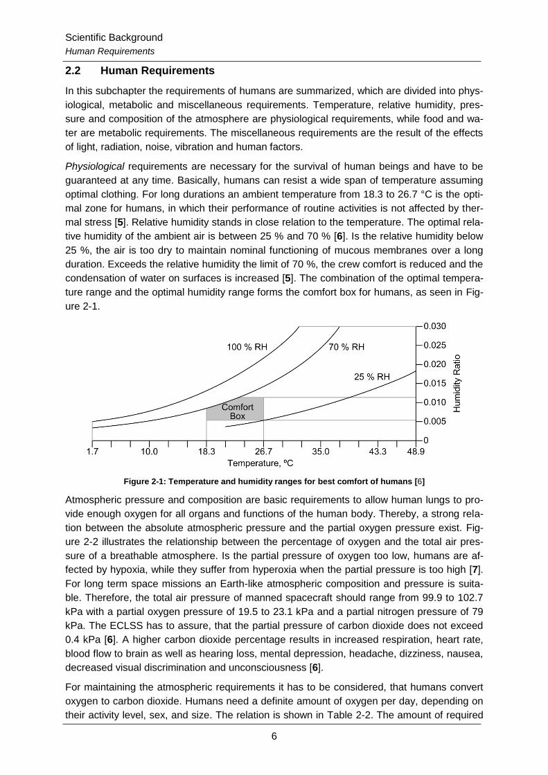
The properties of other planets and moons and the conditions on their surfaces vary from the
Earth’s. Moon and Mars are probable targets for the first long-time or even permanent
crewed base. Therefore, this subchapter describes the properties and environmental condi-
tions of Moon and Mars and compares the conditions to that on Earth. The general proper-
ties, the magnetic field, the radiation, the atmosphere, the surface temperature as well as the
composition of the local soil are discussed. A comparison of properties between Earth, Moon
and Mars is shown in Table 2-1.
The Moon is the sole natural satellite orbiting around Earth. According to reference [2], he
has a radius of 1738 kilometers and surrounds the Earth in a mean distance of 384400 kilo-
meters in 27.32 days. The Moon’s gravity constant has a value of 1.62 m/s2; this is around
one sixth of the Earth’s. Earth and Moon have the same mean distance from the Sun; hence
both have the same mean solar constant of 1368 W/m2. However, opposed to Earth the
Moon’s day and night at the equator have a length of 14 Earth days each [1]. The poles of
the Moon are subject to a half-year day-night-cycle. Due to the low gravity, the Moon cannot
maintain an atmosphere. The temperature on the surface at the equator ranges from 120 °K
during night to 380 °K during day [2]. Nevertheless, at the poles the temperature can fall to
40 °K in permanently shaded craters [1]. As a consequence of absent atmosphere and mag-
netic field, the Moon receives twice as much UV radiation the Earth does and a higher
amount of ionizing radiation. The lunar soil consists of 42 % oxygen, 21 % silicone, 13 %
iron, 8 % calcium, 7 % aluminum and 6 % magnesium. Usually, these elements are bound in
Scientific Background
Environmental Conditions
5
oxides. Basically it is feasible to extract hydrogen, oxygen, water and other useful materials
out of the soil, but the processes require either high power or high temperatures [1].
Mars is the fourth planet of our solar system as seen from sun. He surrounds the Sun in
686.98 days in a distance of 1.54 AU [1]. Phobos and Demios are the names of the two
moons orbiting around the Mars. The Martian equatorial radius is around 3396 kilometers.
Due to the higher distance from the Sun, the mean intensity of the solar radiation is 615
W/m2. However, the orbit of Mars is more eccentric than the Earth’s; hence the solar con-
stant varies from 493 W/m2 at aphelion to 718 W/m2 at perihelion [1]. Mars possesses a thin
atmosphere consisting of 95.3 % carbon dioxide, 2.7 % nitrogen and 1.6 % argon. The mean
surface pressure of the atmosphere is around 6 mbar [3]. The mean surface temperature is
210 °K, but the temperature varies from 130 °K to 300 °K, depending on the region [1]. Due
to the thin atmosphere and the low concentration of ozone, the UV radiation reaching the
Martian surface is higher than reaching the surface of the Earth. Mars maintains a magnetic
field, but it is not strong enough to keep the particles of ionizing radiation outside the atmos-
phere. The atmosphere itself provides protection against ionizing radiation, but the level of
protection varies with the composition and dimension of the atmosphere [1]. The Martian soil
consists of 43 % oxygen, 21 % silicone, 13 % iron, 8 % potassium, 5 % magnesium, 4 % cal-
cium, 3 % aluminum and 3 % sulfur [1].
Table 2-1: Properties of Earth, Moon and Mars
Earth Moon Mars
Equatorial Radius 6378 km 1738 km 3396 km
Mean Surface Gravity 9.81 m/s2 1.62 m/s
2 3.72 m/s
2
Mean Distance from Sun 149.6 * 106 km 149.6 * 10
6 km 227.9 * 10
6 km
Mean Solar Constant 1368 W/m2 1368 W/m
2 615 W/m
2
Atmospheric Composition 78 % N2
21 % O2
0.93 % CO2
none 95.3 % CO2
2.7 % N2
1.6 % Ar
Mean Surface Pressure 1 bar 3 * 10-15
bar 0.006 bar
Mean Surface Temperature 288 °K day: 380 °K
night: 120 °K
210 °K
Reference [4] [2] [3]
Scientific Background
Human Requirements
6
2.2 Human Requirements
In this subchapter the requirements of humans are summarized, which are divided into phys-
iological, metabolic and miscellaneous requirements. Temperature, relative humidity, pres-
sure and composition of the atmosphere are physiological requirements, while food and wa-
ter are metabolic requirements. The miscellaneous requirements are the result of the effects
of light, radiation, noise, vibration and human factors.
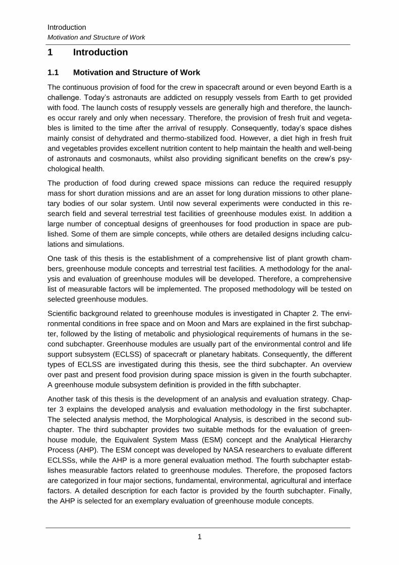
Physiological requirements are necessary for the survival of human beings and have to be
guaranteed at any time. Basically, humans can resist a wide span of temperature assuming
optimal clothing. For long durations an ambient temperature from 18.3 to 26.7 °C is the opti-
mal zone for humans, in which their performance of routine activities is not affected by ther-
mal stress [5]. Relative humidity stands in close relation to the temperature. The optimal rela-
tive humidity of the ambient air is between 25 % and 70 % [6]. Is the relative humidity below
25 %, the air is too dry to maintain nominal functioning of mucous membranes over a long
duration. Exceeds the relative humidity the limit of 70 %, the crew comfort is reduced and the
condensation of water on surfaces is increased [5]. The combination of the optimal tempera-
ture range and the optimal humidity range forms the comfort box for humans, as seen in Fig-
ure 2-1.
Figure 2-1: Temperature and humidity ranges for best comfort of humans [6]
Atmospheric pressure and composition are basic requirements to allow human lungs to pro-
vide enough oxygen for all organs and functions of the human body. Thereby, a strong rela-
tion between the absolute atmospheric pressure and the partial oxygen pressure exist. Fig-
ure 2-2 illustrates the relationship between the percentage of oxygen and the total air pres-
sure of a breathable atmosphere. Is the partial pressure of oxygen too low, humans are af-
fected by hypoxia, while they suffer from hyperoxia when the partial pressure is too high [7].
For long term space missions an Earth-like atmospheric composition and pressure is suita-
ble. Therefore, the total air pressure of manned spacecraft should range from 99.9 to 102.7
kPa with a partial oxygen pressure of 19.5 to 23.1 kPa and a partial nitrogen pressure of 79
kPa. The ECLSS has to assure, that the partial pressure of carbon dioxide does not exceed
0.4 kPa [6]. A higher carbon dioxide percentage results in increased respiration, heart rate,
blood flow to brain as well as hearing loss, mental depression, headache, dizziness, nausea,
decreased visual discrimination and unconsciousness [6].
For maintaining the atmospheric requirements it has to be considered, that humans convert
oxygen to carbon dioxide. Humans need a definite amount of oxygen per day, depending on
their activity level, sex, and size. The relation is shown in Table 2-2. The amount of required

Scientific Background
Human Requirements
7
oxygen ranges from 0.52 to 1.11 kg per person and day [8]. The carbon dioxide output of
humans is between 0.726 and 1.226 kg per person and day [6].
Figure 2-2: Breathable percentage of oxygen as a function of total pressure [7]
The metabolic requirements are demands of humans for missions that last longer than a few
hours. The metabolic load of a person depends on his/her activity level, sex and, age, body
mass and height. Exemplary values for the metabolic load of different activity levels are
shown in Table 2-2. However, the metabolic load is calculated with the equation for the En-
ergy Efficiency Ratio (EER) for men 19 years and older [5]:
[ ⁄ ] [ ] ( [ ]
[ ]) (1)
and for women 19 years and older with the equation:
[ ⁄ ] [ ] ( [ ]
[ ]) (2)
Table 2-2: Human metabolic load and oxygen requirements [8]
Activity level
Metabolic Load
[kcal/(CM*d)]
Oxygen Requirements
[kg/(CM*d)]
Low Activity 2618 0.78
Nominal Activity 2822 0.84
High Activity 3223 0.96
5th Percentile Nominal
Female 1812 0.52
95th Percentile Nominal
Male 3718 1.11
The demands of water and food per day depend on the metabolic load. According to refer-
ence [8], the daily fluid intake can be assumed from 1.0 to 1.5 milliliters per kcal. However,
the minimum fluid intake has to be at least 2 liters per person and day. Reference [5] de-
clares, that 50 to 55 % of the daily energy intake shall be provided by carbohydrates. There-
Scientific Background
Environmental Control and Life Support Systems
8
by, complex carbohydrates (e.g. starches) have to be preferred and simple sugars should not
exceed 10 % of the total carbohydrate intake. Furthermore, 12 to 15 % [8] and not more
than 35 % [5] of the daily energy intake has to be delivered by proteins. The suitable ratio of
animal and plant based proteins is 3:2. Higher and lower intakes of proteins can amplify
space-induced musculoskeletal changes. The daily energy intake provided by fat should
range from 25 to 35 % [5] with a ratio of 1:1.5 to 2:1 for polysaturated, monosaturated and
saturated fat [8]. A detailed compilation of the daily energy intake through macronutrients
(carbohydrates, protein, fat, cholesterol and fiber) is shown in Appendix 2-1. In addition to
macronutrients humans require several micronutrients like vitamins and minerals. A detailed
list of the recommended intake of them is shown in Appendix 2-2: Recommended Micronutri-
ent Daily Dietary Intake. Altogether each person needs 0.5 to 0.86 kg (dry mass) food per
day [6].
Besides the physiological and metabolic requirements are others, which are grouped under
miscellaneous requirements. The necessities of humans for light, radiation shielding, noise
and vibration protection as well as human factors are part of this group. The description of
these requirements is neglected by this thesis. However, the references [5] and [8] provide
further information about this topic.
2.3 Environmental Control and Life Support Systems
The Environmental Control and Life Support System (ECLSS) is a subsystem of crewed
spacecraft. The task of the ECLSS is the maintenance of all human requirements, as dis-
cussed in the previous subchapter, to assure the survival, optimal work performance and
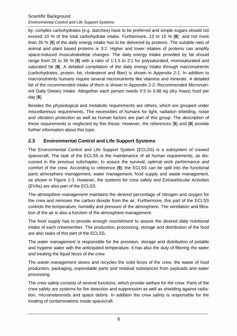
comfort of the crew. According to reference [9], the ECLSS can be split into the functional
parts atmosphere management, water management, food supply and waste management,
as shown in Figure 2-3. However, the systems for crew safety and Extravehicular Activities
(EVAs) are also part of the ECLSS.
The atmosphere management maintains the desired percentage of nitrogen and oxygen for
the crew and removes the carbon dioxide from the air. Furthermore, this part of the ECLSS
controls the temperature, humidity and pressure of the atmosphere. The ventilation and filtra-
tion of the air is also a function of the atmosphere management.
The food supply has to provide enough nourishment to assure the desired daily nutritional
intake of each crewmember. The production, processing, storage and distribution of the food
are also tasks of this part of the ECLSS.
The water management is responsible for the provision, storage and distribution of potable
and hygiene water with the anticipated temperature. It has also the duty of filtering the water
and treating the liquid feces of the crew.
The waste management stores and recycles the solid feces of the crew, the waste of food
production, packaging, expendable parts and residual substances from payloads and water
processing.
The crew safety consists of several functions, which provide welfare for the crew. Parts of the
crew safety are systems for fire detection and suppression as well as shielding against radia-
tion, micrometeoroids and space debris. In addition the crew safety is responsible for the
treating of contaminations inside spacecraft.
Scientific Background
Environmental Control and Life Support Systems
9
Figure 2-3: Tasks and interfaces of life support systems [9]
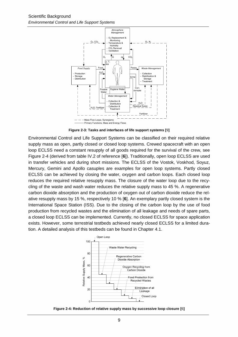
Environmental Control and Life Support Systems can be classified on their required relative
supply mass as open, partly closed or closed loop systems. Crewed spacecraft with an open
loop ECLSS need a constant resupply of all goods required for the survival of the crew, see
Figure 2-4 (derived from table IV.2 of reference [6]). Traditionally, open loop ECLSS are used
in transfer vehicles and during short missions. The ECLSS of the Vostok, Voskhod, Soyuz,
Mercury, Gemini and Apollo casuples are examples for open loop systems. Partly closed
ECLSS can be achieved by closing the water, oxygen and carbon loops. Each closed loop
reduces the required relative resupply mass. The closure of the water loop due to the recy-
cling of the waste and wash water reduces the relative supply mass to 45 %. A regenerative
carbon dioxide absorption and the production of oxygen out of carbon dioxide reduce the rel-
ative resupply mass by 15 %, respectively 10 % [6]. An exemplary partly closed system is the
International Space Station (ISS). Due to the closing of the carbon loop by the use of food
production from recycled wastes and the elimination of all leakage and needs of spare parts,
a closed loop ECLSS can be implemented. Currently, no closed ECLSS for space application
exists. However, some terrestrial testbeds achieved nearly closed ECLSS for a limited dura-
tion. A detailed analysis of this testbeds can be found in Chapter 4.1.
Figure 2-4: Reduction of relative supply mass by successive loop closure [6]

Scientific Background
Survey on Past and Present Food Provision in Crewed Spacecraft
10
Closure of the individual loops can be achieved with Physico-Chemical (P/C) or Biological
Life Support Systems (BLSS). Physico-chemical life support systems use physical or chemi-
cal processes to fulfill the tasks of an ECLSS. They are capable of accomplishing the tasks
of the atmosphere, water and waste management and close the water and oxygen loop [10].
Several technologies for P/C life support systems exist. Available P/C systems for the water
management are shown in Appendix 2-3: P/C Technologies for the Water Management,
while P/C technologies for air revitalization are shown in Appendix 2-4: P/C Technologies for
Air Revitalization. P/C systems are not capable to produce food, therefore, biological sys-
tems are necessary. A BLSS uses plants, algae or other creatures to produce food and fulfill
the tasks of the atmosphere, water and waste management. However, the design and opera-
tion of a BLSS is complex and the mass of such systems is high. When a combination of P/C
systems and BLSS are used in a crewed spacecraft, the ECLSS is a hybrid system, while a
life support system containing only BLSS is called Controlled Ecological Life Support System
(CELSS). Figure 2-5 shows the cumulative mass of different forms of ECLSS as a function of
the mission duration, and the break even points at which one system is more suitable than
another [11].
Figure 2-5: Cumulative mass of different ECLSS as a function of mission duration [11]
Hence, nonregenerable systems are only applicable for short duration missions, regenerable
P/C systems are suitable for mid duration mission, and hybrid or CELSS are required for long
duration missions like permanent bases on other planets.
2.4 Survey on Past and Present Food Provision in Crewed Spacecraft
The food provision for humans in crewed spacecraft changed in the past decades with the
increasing mission duration. This subchapter illustrates the evolution of food provision sys-
tems from Apollo to the space stations Mir and ISS. According to reference [12], the provi-
sion of high nutritional, well-balanced food for all members of the crew is important to assure
their welfare and possibility to work in space and during Extravehicular Activities (EVAs).
Food for astronauts has to be easy to prepare, but still attractive to eat. Furthermore, the
food must be small in volume, low in weight and low in waste to reduce launch and operation
costs. Besides the delivery of nutrients, food preparation, cooking and eating together are
important social events for the crew of spacecraft. Therefore, a suitable eating place is re-
quired inside the spacecraft [12].

Scientific Background
Survey on Past and Present Food Provision in Crewed Spacecraft
11
The Apollo spacecraft were designed for crewed missions to the Moon, including a landing
and EVAs on the lunar surface. The crew of an Apollo mission consisted of three astronauts;
two of them were assigned for the lunar surface mission segment. The whole mission time
was supposed to be not longer than 14 days. The food system design for the Apollo space-
craft was based on the experiences of the Mercury and Gemini programs [12]. Food during
the Apollo missions was available in four different forms, bite-sized, rehydratables and semi-
solid thermostabilized food, and beverage powder. The bite-sized food was dehydrated small
cubes with different tastes like meat, cheese and fruits. The cubes were rehydrated with sali-
va inside the mouth. Rehydratables were precooked and dehydrated meals, which could be
rehydrated with water in less than 15 minutes. Tuna, salmon or chicken salads, and shrimp
cocktail were available as rehydratables. The semisolid thermostabilized food was served in
flexible metal tubes and consisted of high-nutrient fluids. Figure 2-6 shows a typical Apollo
food package. Inside the Apollo spacecraft was no dedicated area for food preparation and
consumption. However, the food provision evolved during the Apollo program. During later
missions new kinds of flavors were introduced and sandwiches were available too [12].
The food for the Soviet Salyut missions was prepared to last up to 18 months and consisted
primarily of canned, dehydrated and in aluminum tubes stored meals. The meals rotated in a
six day cycle. In addition to the food the cosmonauts took vitamin pills. Fresh food was
sometimes provided by visiting crews. During the Salyut missions several small plant growth
chambers were tested for the usage of growing fresh food in space [12]. The food of the Sal-
yut program has improved over time. From Salyut 7 on a pantry system replaced the pre-
cooked and packed food. A folding table for preparing and eating food was installed inside
the work compartment. Two electrical ovens and tools for the meal preparation were also in-
cluded in the eating table. Furthermore, the cosmonauts were allowed to select their food by
themselves within a calculated caloric ratio [12].
According to reference [12], the American Skylab space station had a dedicated food pro-
cessing and eating area, the wardroom. Figure 2-7 shows the Skylab food tray, which could
be placed into a table inside the wardroom, which was located in the center, so that all three
crewmembers could eat together at the same time. In addition to the table and food prepar-
ing tools, the wardroom had a freezer and a refrigerator. The astronauts were able to select
their food from rehydratables, thermostabilized and frozen meals. Beverages were also
available. Each astronaut had his own food tray, where they could heat their meals individu-
ally. The trays consisted of four small and four large openings for holding the food packages,
and one opening to hold a plastic bottle filled with beverages. Three of the large openings
were able to heat the food packages [12].
Figure 2-6: Apollo space food [13]
Figure 2-7: Skylab food tray [13]

Scientific Background
Survey on Past and Present Food Provision in Crewed Spacecraft
12
During the missions of the Space Shuttle the food of the astronauts consisted of rehydrata-
bles, thermostabilized, irradiated and fresh food. The astronauts could select their menu
several months before the flight. They were able to combine meals out of over 200 food
items. After the selection, the meals were analyzed on their nutritional content and corrected
by NASA physicians. The usual short mission durations allowed the provision of a variety of
fresh food, such as bread, fruits and vegetables. The fresh food was stored inside the fresh
food locker. Each crewmember had his own locker tray which contained his meals. On the
middeck of the Shuttle a galley rack was installed, which included an oven, a rehydration
unit, a water dispenser for hot and cold water, and the provision of hygiene water. There was
no dedicated eating area inside the Space Shuttle. Astronauts had to use a food service tray
attached to their legs to prepare their food [12], see Figure 2-8.
The food consumed on board the Mir space station was storable for up to 18 months due to
dehydration. Usually, the food was chopped in bite-sized pieces and packed in plastic bags.
The periodic resupply with Progress spacecraft allowed the delivery of fresh food for the Mir
crew. The cosmonauts were allowed to select their food for each day, as long as it met the
nutritional requirements. In addition to the food, vitamins were applied due taking pills. Inside
the Mir base block a food cabinet existed, which included a refrigerator and an eating table.
The table was used to prepare the meals. The Russians continued their research in plant
growth chambers and small greenhouses for space applications. Therefore, several plant
growth chambers were tested aboard the Mir station. These chambers provided some fresh
food for the crew [12].
Figure 2-8: Space Shuttle food tray [13]
Figure 2-9: ISS food container [13]
The ISS food facility is similar to the Mir’s, because of its location inside the Russian Zvezda
module. It consists of a table, hot water dispenser, food storage and heaters. Usually, the
meals are a combination of thermostabilized rehydratables, intermediate moisture, and pre-
cooked, fresh and irradiated food. Beverages are also provided. Each crewmember can cre-
ate an own menu, based on a 16-day rotation. Therefore, several food items from Russia,
USA, Europe and Japan can be combined. In addition to the normal meals, each crewmem-
ber has a bonus container which can be filled with any food that meets the microbiological
requirements [12]. Figure 2-9 shows a filled food container for the ISS.

Scientific Background
Greenhouse Module Subsystems
13
2.5 Greenhouse Module Subsystems
2.5.1 Classification
Comparable to spacecraft, greenhouse modules can be divided into several subsystems.
However, the existing greenhouse module subsystem classifications are not consistent, be-
cause each research team established their own nomenclature. Consequently, this chapter
describes the classification of greenhouse module subsystems used in this thesis. The se-
lected approach is a fundamental classification, in which every subsystem has its own tasks.
Nevertheless, some subsystems could be merged, because of their close relations to each
other.
The ten subsystems of greenhouse modules are the Plant Cultivation Subsystem (PCS), the
Nutrient Delivery Subsystem (NDS), the Harvest & Cleaning Subsystem (HCS), the Atmos-
phere Control Subsystem (ACS), the Water Control Subsystem (WCS), the Lighting Control
Subsystem (LCS), the Thermal Control Subsystem (TCS), the Structures & Mechanisms
Subsystem (SMS), the Power Control & Distribution Subsystem (PCDS) and the Command &
Data Handling Subsystem (CDHS). They can be assigned to three groups of subsystem, as
shown in Figure 2-10. The groups are named Agricultural Subsystems, Environmental Con-
trol Subsystems and Fundamental & Interface Subsystems.
Figure 2-10: Classification of Greenhouse Module Subsystems
2.5.2 Fundamental & Interface Subsystems
The fundamental & interface subsystems are the framework of the greenhouse module. The
Structures and Mechanisms Subsystem, the Power Control & Distribution Subsystem and the
Command & Data Handling Subsystem are part of this subsystem category.
The functions of the Structures & Mechanisms Subsystem (SMS) of greenhouse modules
and spacecraft are similar. According to reference [14], the SMS is the mechanical support of
all other subsystems. The structures have to withstand all applied loads during the whole
mission. In addition the radiation shielding is part of the SMS. Furthermore, the SMS is re-
sponsible for all mechanisms used in greenhouse modules.

Scientific Background
Greenhouse Module Subsystems
14
Unlike the electrical power system (EPS) of spacecraft, the Power Control & Distribution
Subsystem (PCDS) of greenhouse modules does not generate or store electrical power, it
only controls and distributes the electrical power provided by the electrical power system of
the habitat [15]. However, greenhouse modules can contain batteries or other power supply
for cases of emergency. The power demand of greenhouse modules depends on the power
consumption of the other subsystems. In general the Environmental Control Subsystems
have the highest demands, especially the LCS. The PCDS has to supply each of the other
subsystems with the voltage they need, to assure the subsystems can work as desired.
The Command & Data Handling Subsystem (CDHS) of greenhouse modules has to fulfill the
same functions as in every spacecraft: receiving, validating, decoding and distributing of
commands to other subsystems and gathering, processing and formatting of data as well as
data storage. Security interfaces and computer health monitoring are also functions of the
CDHS [16]. Due to maintain optimal growth conditions for plants in greenhouse modules the
CDHS has to interpret the signals of several sensors to send suitable commands to each
subsystem. The higher the level of automation of the greenhouse, the higher is the complexi-
ty of the CDHS. Furthermore, when the CDHS is a physical part of the greenhouse module, it
has to be protected against the high humidity and temperature inside the greenhouse. The
CDHS of greenhouse modules can also be part of the habitat CDHS.
2.5.3 Environmental Control Subsystems
The purpose of the environmental control subsystems is the maintenance of all environmen-
tal conditions, which are required either by humans or plants. Especially the optimal growth
environment is necessary for the plants to achieve a high yield. Usually the subsystems of
this group are combined in the ECLSS of the spacecraft, but it is suitable to split the func-
tions into different subsystems when analyzing greenhouse modules. This subsystem group
consists of the Atmosphere Control Subsystem, the Water Control Subsystem, the Lighting
Control Subsystem and the Thermal Control Subsystem.
The Atmosphere Control Subsystem (ACS) is responsible for the air management of the
greenhouse module. This responsibility covers the monitoring and control of the humidity, the
composition and the pressure of the air. Furthermore, the ACS has to filter the air and has to
assure, that the air circulates through the whole greenhouse module. Especially the humidity
and the air composition have a great impact on the growth rate of plants. Usually, the ACS of
greenhouse modules is connected to the ECLSS of the habitat to allow gas exchange.
The Water Control Subsystem (WCS) monitors and regulates the water distribution and wa-
ter quality. The main task of the WCS is the delivery of the desired amount of water to every
plant in the greenhouse module to achieve an optimal growth rate. The water quality is also
important for the growth rate of plants. The WCS of greenhouse modules have a connection
to the water management system of the habitat. However, the WCS must be capable to store
a defined amount of water for cases of emergency.
The task of the Lighting Control Subsystem (LCS) is to provide and maintain the illumination
of the greenhouse module. Therefore, it must be considered the lighting for the crew and the
lighting for plants. The crew needs light for the work inside the greenhouse module, while
plants need special lighting for an optimal growth rate. The growth rate depends on the light
spectrum, the light intensity and the illumination phases. The required lighting conditions dif-
fer between plant species, consequently the LCS has to provide the optimal lighting condi-
Scientific Background
Greenhouse Module Subsystems
15
tions for each plant species for the maximum yield. When the greenhouse module uses the
sun as a light source, the LCS has to regulate the irradiation of the sunlight.
In spacecraft, the Thermal Control Subsystem (TCS) maintains the temperature of all com-
ponents at every time of the mission within their limits [17]. In general the TCS of greenhouse
modules has to fulfill the same functions. In greenhouse modules the critical elements for the
TCS are the plants. Different plant species have different requirements on the temperature;
consequently, different temperature zones in the greenhouse module can exist and the TCS
has to maintain the requirements of each zone. The thermal insulation of the greenhouse
module is also part of this subsystem. The insulation has to ensure that the heat loss to the
environment and to other parts of the habitat is as low as possible to reduce the energy de-
mand of the TCS. However, depending on the lighting source, special cooling devices are
necessary to protect the plants from overheating.
2.5.4 Agricultural Subsystems
Agricultural subsystems encompass all subsystems directly related to the plants. Parts of this
subsystem group are the Plant Cultivation Subsystem, the Nutrient Delivery Subsystem and
the Harvest & Cleaning Subsystem.
The Plant Cultivation Subsystem (PCS) supports the plants during all development stages.
The PCS contains the growth medium for the plants, the plants themselves and can be di-
vided into root and shoot zone. The design of the PCS is directly affected by the selected
plant cultivation method and the used growth medium. Furthermore, the PCS has to ensure,
that the plants have a solid stand in the growth medium and grow as desired. Generally, the
plant cultivation system consists of several growth units, which are separated from each oth-
er and have their own environmental conditions and nutrient composition depending on the
plant species and development stage.
The Nutrient Delivery Subsystem (NDS) is responsible for the mixture of the plants’ nutrients.
As every plant species has other requirements concerning the nutrients, a special nutrient
mixing system is required. The nutrient solution has to be distributed to every plant in the
greenhouse module in the desired amount and composition. The storage of nutrients is also
part of the NDS. Furthermore, the nutrient production can be part of the NDS of greenhouse
modules, but usually this task is fulfilled by the waste treatment system of the habitat.
The task of the Harvest & Cleaning Subsystem (HCS) is the provision of all tools and materi-
als that are necessary for harvesting and cleaning the cultivated plants. Therefore, the HCS
has to have a waste storage system to temporarily store the inedible parts of plants, before
they are distributed to the waste treatment system of the habitat. The crop gathered from
plants has to be packed after the harvesting and cleaning procedure. Consequently, the HCS
has to provide the tools for the packaging. Afterwards the packed crop has to be stored.
Scientific Background
Summary
16
2.6 Summary
Chapter 2 presents a brief overview over the required scientific background for the analysis
and evaluation of greenhouse modules within planetary outposts. The challenges of the envi-
ronmental conditions in free space, on Moon and on Mars are described.
Furthermore, the human requirements are discussed with respect to the required amount of
food, water and oxygen. In addition the atmospheric pressure, composition and relative hu-
midity required for long duration missions are explained.
The third subchapter discusses the different kinds of Environmental Control and Life Support
Subsystems compared to the mission duration. Consequently, for long duration or even per-
manent missions to other planetary bodies of the solar system, greenhouse modules are a
necessity.
A summary of past and present food provision systems shows the evolution of these systems
over the last decades of spaceflight, from the Apollo program to the ISS.
In the fifth subchapter a classification of all greenhouse module subsystems is established.
Therefore, each category and the related subsystems are described. In addition the functions
and tasks associated with each subsystem are explained.
Development of an Analysis and Evaluation Strategy
Methodology
17
3 Development of an Analysis and Evaluation Strategy
This chapter starts with the explanation of the methodology of the developed analysis and
evaluation strategy in the first subchapter. In the second subchapter the chosen analysis
method, the Morphological Analysis (MA) is described, followed by the explanation of two
suitable evaluation methods in the third subchapter. The fourth subchapter describes the
analysis and evaluation factors considered during this thesis.
3.1 Methodology
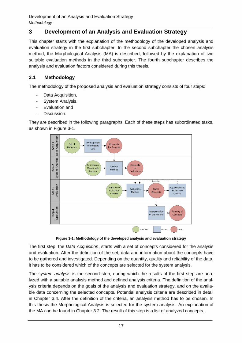
The methodology of the proposed analysis and evaluation strategy consists of four steps:
- Data Acquisition,
- System Analysis,
- Evaluation and
- Discussion.
They are described in the following paragraphs. Each of these steps has subordinated tasks,
as shown in Figure 3-1.
Figure 3-1: Methodology of the developed analysis and evaluation strategy
The first step, the Data Acquisition, starts with a set of concepts considered for the analysis
and evaluation. After the definition of the set, data and information about the concepts have
to be gathered and investigated. Depending on the quantity, quality and reliability of the data,
it has to be considered which of the concepts are selected for the system analysis.
The system analysis is the second step, during which the results of the first step are ana-
lyzed with a suitable analysis method and defined analysis criteria. The definition of the anal-
ysis criteria depends on the goals of the analysis and evaluation strategy, and on the availa-
ble data concerning the selected concepts. Potential analysis criteria are described in detail
in Chapter 3.4. After the definition of the criteria, an analysis method has to be chosen. In
this thesis the Morphological Analysis is selected for the system analysis. An explanation of
the MA can be found in Chapter 3.2. The result of this step is a list of analyzed concepts.

Development of an Analysis and Evaluation Strategy
Analysis Method – The Morphological Analysis
18
At the beginning of the third step, the evaluation, the analyzed concepts of the previous step
has to be split into different groups of concepts, depending on their purpose. Only concepts
with the same purpose can be evaluated and compared to each other. To evaluate the con-
cepts, evaluation criteria has to be defined. Usually, these criteria are a subset of the analy-
sis criteria. Various evaluation methods exist and the analyst has to select an appropriate
method. During this thesis the Equivalent System Mass (ESM) and the Analytical Hierarchy
Process (AHP) are considered to be suitable for the evaluation of greenhouse module con-
cepts. Both methods are described in Chapter 3.3. The output of the evaluation step is a list
of rated concepts. However, when the result does not fit to the expected outcome or other
reasons exist, the evaluation criteria and method can be adjusted. When adjustments are
made, the evaluation has to be repeated.
In the fourth step, the discussion, the results of the analysis and evaluation have to be
checked on their consistency and interpreted by the analyst. The outcome of this step of the
strategy is a ranking of the investigated concepts.
3.2 Analysis Method – The Morphological Analysis
The Morphological Analysis was developed “by Fritz Zwicky, the famous astrophysicist and
jet engine pioneer, to describe a technique for identifying, indexing, counting, and parameter-
izing the collection of all possible devices to achieve a specified functional capability.” [18]
According to reference [19], the procedure of a MA consists of four phases:
Phase 1: Formulation of the problem,
Phase 2: Identification of all characteristic parameters,
Phase 3: Subdivision of each parameter into all possible options,
Phase 4: Analysis and evaluation of all possible parameter-option combinations.
In the first phase a precise formulation of the problem or the wanted functional capability has
to be established.
In the second phase, the identification of all characteristic parameters, all parameters which
affect the problem have to be identified.
During the third phase of the MA, the subdivision of each parameter into all possible options,
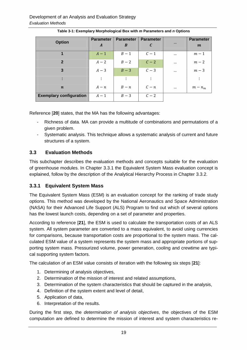
the Morphological Box is constructed. The Morphological Box is the main tool of the MA and
visualizes all parameters and their options in a table. The options have to be carefully select-
ed, so that only one option per parameter is feasible at the same time. An exemplary box is
shown in Table 3-1. A number of possible options exist for each parameter . The green
highlighted options in Table 3-1 form one out of possible configurations.
Usually the fourth phase, the analysis and evaluation of all possible parameter-option com-
binations, is done by a separate evaluation method. The number of combinations for a giv-
en Morphological Box can be calculated by multiplying the number of options of each param-
eter. For the example in Table 3-1 the formula is:
. (3)
Development of an Analysis and Evaluation Strategy
Evaluation Methods
19
Table 3-1: Exemplary Morphological Box with m Parameters and n Options
Option Parameter
Parameter
Parameter
Parameter
1
2
3
Exemplary configuration
Reference [20] states, that the MA has the following advantages:
- Richness of data. MA can provide a multitude of combinations and permutations of a
given problem.
- Systematic analysis. This technique allows a systematic analysis of current and future
structures of a system.
3.3 Evaluation Methods
This subchapter describes the evaluation methods and concepts suitable for the evaluation
of greenhouse modules. In Chapter 3.3.1 the Equivalent System Mass evaluation concept is
explained, follow by the description of the Analytical Hierarchy Process in Chapter 3.3.2.
3.3.1 Equivalent System Mass
The Equivalent System Mass (ESM) is an evaluation concept for the ranking of trade study
options. This method was developed by the National Aeronautics and Space Administration
(NASA) for their Advanced Life Support (ALS) Program to find out which of several options
has the lowest launch costs, depending on a set of parameter and properties.
According to reference [21], the ESM is used to calculate the transportation costs of an ALS
system. All system parameter are converted to a mass equivalent, to avoid using currencies
for comparisons, because transportation costs are proportional to the system mass. The cal-
culated ESM value of a system represents the system mass and appropriate portions of sup-
porting system mass. Pressurized volume, power generation, cooling and crewtime are typi-
cal supporting system factors.
The calculation of an ESM value consists of iteration with the following six steps [21]:
1. Determining of analysis objectives,
2. Determination of the mission of interest and related assumptions,
3. Determination of the system characteristics that should be captured in the analysis,
4. Definition of the system extent and level of detail,
5. Application of data,
6. Interpretation of the results.
During the first step, the determination of analysis objectives, the objectives of the ESM
computation are defined to determine the mission of interest and system characteristics re-
Development of an Analysis and Evaluation Strategy
Evaluation Methods
20
lated to the trade study. Furthermore, the objectives have to be defined in an appropriate
level of detail to avoid complications during the computation.
The second step, the determination of the mission of interest and related assumptions, is
used to make assumptions about the operating environment, the subsystem of interest and
the surrounding system. NASA defines several assumptions and missions of interest in two
reports: the Advanced Life Support Systems Integration, Modeling, and Analysis Reference
Missions Document (ALS RMD, [22]) and the Advanced Life Support Baseline Values and
Assumptions Document (ALS BVAD, [23]).
According to reference [21], the determination of the system characteristics that should be
captured in the analysis is the third step in the process of calculating an ESM value. During
this step the analyst decides which characteristics are investigated during the trade study
based upon the objectives. Characteristics might be excluded from the study due to a lack of
data or other means. Usually, the characteristics are based upon the function, the availability,
the gravity dependence, the noise levels, the safety, the radiation susceptibility or other pa-
rameters of the investigated system.
In the fourth step, the definition of the system extent and level of detail, the analyst has to
define the investigated systems to a level of detail necessary for an appropriate comparison
of the characteristics of interest between the systems. However, functional differences be-
tween the system options can complicate the identification of a suitable level of detail for the
calculation of an ESM value.
The application of data, the sixth step, is necessary to adjust the data gathered from re-
searchers, technology developers or scientific publications for the evaluation with the ESM
method. Reference [21] states the development status adjustment and the system scaling as
the most common types of data modification in an ESM analysis. However, data adjustments
are not limited to both of these. To achieve a reliable result with an ESM evaluation, all study
options have to be normalized to the same development state. Therefore, the analyst has to
assume the future development and the essential parameters of a technology. Usually, data
received from researchers and system developers has to be scaled to an appropriate size for
the ESM study. The scaling factor commonly is a system specific parameter like the mass
flow rate. After determining the scaling factor, all parameter values of the investigated system
have to be adjusted. However, some systems can require more than one scaling factor.
The interpretation of the results is the final step in the ESM process. All results of the proce-
dure have to be interpreted and described in an appropriate style concerning all assumptions
made during the ESM calculation.
The ESM of a system is calculated as the sum of the ESM of each subsystem of the system
of interest. The parameters required for the ESM equation:
∑ [( ) ( ) ( ) ( ) ( )
( ) ( )] , (4)
are shown in Table 3-2.
The initial mass consists of any mass in subsystem i, that is not time- or event-dependent
and not part of the volume, power and cooling terms. The mass for the structure of pressur-
ized volume, for the generation of power and for the provision of cooling is accounted in the
associated terms. The initial volume parameter pertains any pressurized volume required

Development of an Analysis and Evaluation Strategy
Evaluation Methods
21
to house and access subsystem i. The parameter for the required power of subsystem i is .
The cooling term pertains the heat rejection required for subsystem i. is the parameter
for the crewtime required to operate and maintain subsystem i. The time- or event-dependent
mass consists of any mass that is dependent on the mission duration and progress.
Consumables, spare parts and process expendables are examples for this mass term. The
time- or event-dependent volume is the required pressurized volume associated
with . The stowage factors and pertain all equipment required to secure the
system, which can be racks, trays or other equipment. The equivalency factors , ,
and are the ratio of the resource cost, in units of mass, to resource use. In the ALS
BVAD document ( [23]) numerical values and assumptions for the calculation of the stowage
and equivalency factors can be found.
The reliability of an ESM analysis depends on the accuracy of the input data used for the
calculation of the ESM value, as well as on the modification of the data. The ESM evaluation
method is a cost metric. Therefore, the ESM is not capable of taking into account the reliabil-
ity, safety and performance of the investigated systems. Furthermore, it is not feasible to
evaluate qualitative properties of a system with the ESM equation. Consequently, reference
[21] concludes that the ESM concept should not be the only evaluation method used to com-
pare and evaluate trade study options.
Table 3-2: Explanation of ESM equation parameter [21]
Parameter Unit Name
kg Equivalent System Mass value
kg Initial mass of subsystem i
kg/kg Initial mass stowage factor for subsystem i
m3 Initial volume of subsystem i
kg/m3
Mass equivalency factor for the pressurized volume support infrastructure
of subsystem i
kWe Power requirement of subsystem i
kg/kWe Mass equivalency factor for the power generation support infrastructure
of subsystem i
kWth Cooling requirement of subsystem i
kg/kWth Mass equivalency factor for the cooling infrastructure of subsystem i
CM-h/y Crewtime requirement of subsystem i
D y Duration of the mission segment of interest
kg/CM-h Mass equivalency factor for the Crewtime of subsystem i
kg/y time- or event-dependent mass of subsystem i
kg/kg time- or event-dependent mass stowage factor of subsystem i
m3 time- or event-dependent volume of subsystem i
Development of an Analysis and Evaluation Strategy
Evaluation Methods
22
3.3.2 Analytical Hierarchy Process
The Analytic Hierarchy Process (AHP) was developed by T. L. Saaty in the 1970s and is
used in multiple criteria decision making problems. It involves the reduction of complex deci-
sions to a series of pairwise comparisons. After synthesizing the results, decision-makers
arrive at the best decision with a clear rationale for that decision.
According to reference [24], the AHP can be divided into six steps:
1. Illustration of the decision making problem,
2. Pairwise comparison of criteria,
3. Ranking of the criteria and alternatives,
4. Verification of the consistency of the evaluation,
5. Interpretation of the results,
6. Sensitivity analysis of the results.
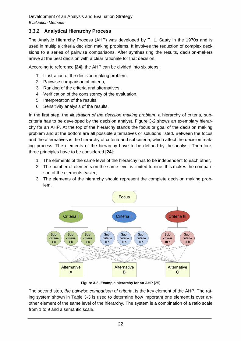
In the first step, the illustration of the decision making problem, a hierarchy of criteria, sub-
criteria has to be developed by the decision analyst. Figure 3-2 shows an exemplary hierar-
chy for an AHP. At the top of the hierarchy stands the focus or goal of the decision making
problem and at the bottom are all possible alternatives or solutions listed. Between the focus
and the alternatives is the hierarchy of criteria and subcriteria, which affect the decision mak-
ing process. The elements of the hierarchy have to be defined by the analyst. Therefore,
three principles have to be considered [24]:
1. The elements of the same level of the hierarchy has to be independent to each other,
2. The number of elements on the same level is limited to nine, this makes the compari-
son of the elements easier,
3. The elements of the hierarchy should represent the complete decision making prob-
lem.
Figure 3-2: Example hierarchy for an AHP [25]
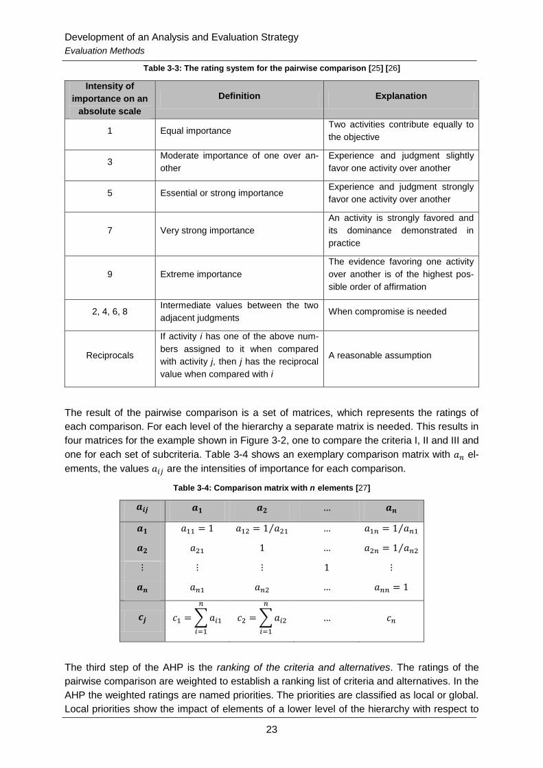
The second step, the pairwise comparison of criteria, is the key element of the AHP. The rat-
ing system shown in Table 3-3 is used to determine how important one element is over an-
other element of the same level of the hierarchy. The system is a combination of a ratio scale
from 1 to 9 and a semantic scale.
Development of an Analysis and Evaluation Strategy
Evaluation Methods
23
Table 3-3: The rating system for the pairwise comparison [25] [26]
Intensity of
importance on an
absolute scale
Definition Explanation
1 Equal importance Two activities contribute equally to
the objective
3 Moderate importance of one over an-
other
Experience and judgment slightly
favor one activity over another
5 Essential or strong importance Experience and judgment strongly
favor one activity over another
7 Very strong importance
An activity is strongly favored and
its dominance demonstrated in
practice
9 Extreme importance
The evidence favoring one activity
over another is of the highest pos-
sible order of affirmation
2, 4, 6, 8 Intermediate values between the two
adjacent judgments When compromise is needed
Reciprocals
If activity i has one of the above num-
bers assigned to it when compared
with activity j, then j has the reciprocal
value when compared with i
A reasonable assumption
The result of the pairwise comparison is a set of matrices, which represents the ratings of
each comparison. For each level of the hierarchy a separate matrix is needed. This results in
four matrices for the example shown in Figure 3-2, one to compare the criteria I, II and III and
one for each set of subcriteria. Table 3-4 shows an exemplary comparison matrix with el-
ements, the values are the intensities of importance for each comparison.
Table 3-4: Comparison matrix with n elements [27]
⁄ ⁄
⁄
∑
∑
The third step of the AHP is the ranking of the criteria and alternatives. The ratings of the
pairwise comparison are weighted to establish a ranking list of criteria and alternatives. In the
AHP the weighted ratings are named priorities. The priorities are classified as local or global.
Local priorities show the impact of elements of a lower level of the hierarchy with respect to
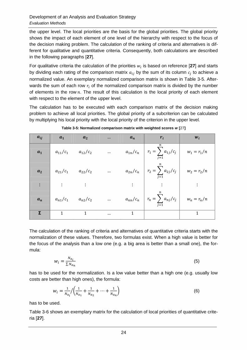
Development of an Analysis and Evaluation Strategy
Evaluation Methods
24
the upper level. The local priorities are the basis for the global priorities. The global priority
shows the impact of each element of one level of the hierarchy with respect to the focus of
the decision making problem. The calculation of the ranking of criteria and alternatives is dif-
ferent for qualitative and quantitative criteria. Consequently, both calculations are described
in the following paragraphs [27].
For qualitative criteria the calculation of the priorities is based on reference [27] and starts
by dividing each rating of the comparison matrix by the sum of its column to achieve a
normalized value. An exemplary normalized comparison matrix is shown in Table 3-5. After-
wards the sum of each row of the normalized comparison matrix is divided by the number
of elements in the row . The result of this calculation is the local priority of each element
with respect to the element of the upper level.
The calculation has to be executed with each comparison matrix of the decision making
problem to achieve all local priorities. The global priority of a subcriterion can be calculated
by multiplying his local priority with the local priority of the criterion in the upper level.
Table 3-5: Normalized comparison matrix with weighted scores w [27]
⁄ ⁄ ⁄ ∑ ⁄
⁄
⁄ ⁄ ⁄ ∑ ⁄
⁄
⁄ ⁄ ⁄ ∑ ⁄
⁄
Σ
The calculation of the ranking of criteria and alternatives of quantitative criteria starts with the
normalization of these values. Therefore, two formulas exist. When a high value is better for
the focus of the analysis than a low one (e.g. a big area is better than a small one), the for-
mula:
∑
(5)
has to be used for the normalization. Is a low value better than a high one (e.g. usually low
costs are better than high ones), the formula:
(
)⁄ (6)
has to be used.
Table 3-6 shows an exemplary matrix for the calculation of local priorities of quantitative crite-
ria [27].

Development of an Analysis and Evaluation Strategy
Evaluation Methods
25
Table 3-6: Weighted and overall alternative scores [27]
Σ
According to reference [24], during the fourth step, the verification of the consistency of the
evaluation, the calculated scores of the previous step are checked on their consistency.
Evaluations are consistent, when the requirements dominance, transitivity and invariance are
met. The fulfillment of the dominance requirement is achieved, when the alternative with the
best rank is presented as the solution of the decision making problem. The invariance cannot
be verified in the AHP. Consequently, the verification of the consistency of the evaluation of
the AHP contains the testing of the transitivity. The more elements are in the hierarchy, the
more complicate is the fulfillment of the requirement.
The calculation of the inconsistency is based on the calculation of the eigenvalue of each el-
ement and is described in detail in reference [27]. However, a short description of the calcu-
lation procedure is described in the following. The first step is the calculation of the eigenval-
ue of each element. Therefore, the mean value has to be calculated for each element. Af-
terwards, the mean value is used to determine the eigenvalues , see Table 3-7.
Table 3-7: Mean matrix and eigenvalue of each element [27]
∑
⁄
∑
⁄
∑
⁄
A decision is consistent, when the maximum eigenvalue is equal to the number of ele-
ments . When the maximum eigenvalue is greater than the number of element, inconsisten-
cy exists. The maximum eigenvalue is calculated with the formula:
∑
. (7)
The consistency index can be calculated out of the maximum eigenvalue and the number
of elements:
. (8)
To judge whether a discrepancy can be tolerated, the consistency relationship is estab-
lished as the division of the consistency index and the random consistency :

Development of an Analysis and Evaluation Strategy
Evaluation Methods
26
. (9)
The random consistency is given as a function of the size of the matrix, see Table 3-8. Dis-
crepancies can be tolerated, when is achieved. Is , the evaluation and/or
the hierarchy has to be reviewed.
Table 3-8: Random consistency R as a function of the size of the matrix [27]
Size of the
matrix 1 2 3 4 5 6 7 8 9 10
Random
consistency R 0.00 0.00 0.52 0.89 1.11 1.25 1.35 1.40 1.45 1.49
In the fifth step, the interpretation of the results, it has to be considered, that the AHP is a
subjective decision making tool. The pairwise comparison is based on individual experiences
and knowledge, the layout of the hierarchy also has a big impact on the results of the AHP.
The interpretation itself can be done by several types of diagrams, graphs and tables.
Reference [24] describes the sensitivity analysis of the results as the sixth step in the AHP.
The sensitivity analysis examines the impacts of changes in the weighting of criteria on the
ranking of the alternatives. Due to continuous changing of the weight of each criteria, borders
are determined, at which the ranking of the alternatives changes. The results of the AHP are
steady, when small changes in the weights do not affect the ranking. The values of the pair-
wise comparison have to be reconsidered, when the results are unsteady.
The AHP is an effective evaluation method for the quantitative examination of unstructured
problems, also with the integration of quantitative values. Furthermore, the AHP is a flexible
tool which allows individuals and groups to define problems according to their approvals and
receive a subjectively preferred solution. The incorporation of expert knowledge can lead to
objectivation of the subjective solution. In addition, the AHP permits the revision of the stabil-
ity and consistency of the solution [27].
Reference [27] summarizes the advantages of the AHP as followed:
- Unity: The AHP is single, easy to understand and flexible model for the analysis of
unstructured problems.
- Complexity: The AHP combines deductive and system approaches for the analysis of
complex problems.
- Interdependency: The AHP can handle interdependencies of system elements and
can break existing paradigm.
- Hierarchy Structure: The AHP incorporates the natural cognitive tendency to order
elements in categories and to group similar elements on the same hierarchy
level.
- Measurement: The AHP provides a scale to measure immaterial criteria and a
method for the determination of priorities.
- Consistency: The AHP incorporates the logical consistency of evaluations, which are
used for the determination of priorities.
- Synthesis: The AHP provides a general approximation of the desirability of each
alternative.
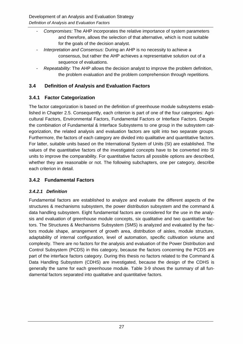
Development of an Analysis and Evaluation Strategy
Definition of Analysis and Evaluation Factors
27
- Compromises: The AHP incorporates the relative importance of system parameters
and therefore, allows the selection of that alternative, which is most suitable
for the goals of the decision analyst.
- Interpretation and Consensus: During an AHP is no necessity to achieve a
consensus, but rather the AHP achieves a representative solution out of a
sequence of evaluations.
- Repeatability: The AHP allows the decision analyst to improve the problem definition,
the problem evaluation and the problem comprehension through repetitions.
3.4 Definition of Analysis and Evaluation Factors
3.4.1 Factor Categorization
The factor categorization is based on the definition of greenhouse module subsystems estab-
lished in Chapter 2.5. Consequently, each criterion is part of one of the four categories: Agri-
cultural Factors, Environmental Factors, Fundamental Factors or Interface Factors. Despite
the combination of Fundamental & Interface Subsystems to one group in the subsystem cat-
egorization, the related analysis and evaluation factors are split into two separate groups.
Furthermore, the factors of each category are divided into qualitative and quantitative factors.
For latter, suitable units based on the International System of Units (SI) are established. The
values of the quantitative factors of the investigated concepts have to be converted into SI
units to improve the comparability. For quantitative factors all possible options are described,
whether they are reasonable or not. The following subchapters, one per category, describe
each criterion in detail.
3.4.2 Fundamental Factors
3.4.2.1 Definition
Fundamental factors are established to analyze and evaluate the different aspects of the
structures & mechanisms subsystem, the power distribution subsystem and the command &
data handling subsystem. Eight fundamental factors are considered for the use in the analy-
sis and evaluation of greenhouse module concepts, six qualitative and two quantitative fac-
tors. The Structures & Mechanisms Subsystem (SMS) is analyzed and evaluated by the fac-
tors module shape, arrangement of growth area, distribution of aisles, module structure,
adaptability of internal configuration, level of automation, specific cultivation volume and
complexity. There are no factors for the analysis and evaluation of the Power Distribution and
Control Subsystem (PCDS) in this category, because the factors concerning the PCDS are
part of the interface factors category. During this thesis no factors related to the Command &
Data Handling Subsystem (CDHS) are investigated, because the design of the CDHS is
generally the same for each greenhouse module. Table 3-9 shows the summary of all fun-
damental factors separated into qualitative and quantitative factors.

Development of an Analysis and Evaluation Strategy
Definition of Analysis and Evaluation Factors
28
Table 3-9: List of Fundamental Factors
Qualitative Factors Quantitative Factors
Module Shape Module Mass
Arrangement of Growth Area Dimensions
Distribution of Aisles Specific Cultivation Volume
Module Structure Complexity
Adaptability of Internal Configura-
tion
Level of Automation
3.4.2.2 Module Shape
Greenhouse modules can have various shapes. The module shape affects the arrangement
of the growth area, the overall growth area and the ratios growth area and growth volume per
total volume. Furthermore, the module mass significantly depends on the shape. Feasible
are:
- prismatic,
- hemispherical,
- spherical or
- irregular
shapes.
Prismatic modules are typically chosen, when the modules are fully integrated on Earth and
launched with rockets. However, the size of prismatic modules integrated on Earth is restrict-
ed to the size of launcher fairings. The base of prisms can be elliptical, polygonal, hemi-
spherical or circular. Today’s modules for space stations are usually prisms with a circular
base, also named cylinders. This results from the aerodynamic cylindrical shape of rockets in
which cylindrical modules have the highest volume efficiency. Due to the experience gained
during the design and construction of space stations in the last decades, prisms and espe-
cially cylindrical ones are a well-known design. Consequently, the development and con-
struction costs for these types are relatively low compared to other shapes.
A hemispherical, or dome like design can be used to cover a big area while keeping the
mass of the construction low. Therefore, a framework of lightweight materials is covered with
a Kevlar based shell. Usually, hemispherical modules are launched as individual components
and have to be assembled at the destination. Consequently, dome greenhouses are only
suitable when a growth area of several hundred square meters is required to feed the crew.
A spherical shape is another option for the design of greenhouse modules. A concept for a
module with a spherical shape was investigated by NASAs Johnson Space Center in 1989 to
be installed at Lacus Veris on Moon [28]. Thereby, an inflatable outer shell was proposed to
form the sphere. The sphere himself was buried half into the lunar, while the upper half was
covered with regolith-filled tubes to protect the crew against radiation. A similar module could
be used as a greenhouse with several floors. An inflatable sphere is light weight and there-
fore, can reduce the launch and transportation costs. However, the sphere has to be enfold-

Development of an Analysis and Evaluation Strategy
Definition of Analysis and Evaluation Factors
29
ed and anchored at the destination which requires a digging device. Furthermore, the sphere
has to be outfitted with the required systems at the destination which causes a high work
load on the crew.
Irregular shapes are theoretically feasible, but until now no concept for a greenhouse module
with an irregular shape exists. However, each design with an irregular shape has to be inves-
tigated in detail on the usefulness for greenhouse modules. When the benefits of the irregu-
lar shape exceed that of regular shapes, it can be considered for greenhouse designs.
3.4.2.3 Arrangement of Growth Area
The arrangement of growth area inside greenhouse modules is an important factor for max-
imizing the yield, because the internal configuration defines the ratios growth area and
growth volume per total volume. The maximum growth height is also affected by the ar-
rangement of growth area. There are several ways to arrange the cultivation area inside
greenhouse modules:
- plain growth area,
- growth area allocated on shelves,
- conveyor like growth area or
- rotating cylinder.
The simplest type of arrangement is a plain growth area, which is similar to the field agricul-
ture on Earth. The volume efficiency of this arrangement is low, because the growth height of
most of the food plants is lower than one meter. Therefore, a field like growth area is less
suitable for extraterrestrial greenhouse modules. A plain growth area is only applicable for
tall growing plants like trees or bushes, but these plants are less considered for the use in
space until now.
Shelf configurations are stacked plain growth areas. Consequently, the ratio of growth vol-
ume per total volume is significantly higher compared to plain growth area configurations.
The height of the different levels of the shelf can vary, so that plants with different growth
heights can be cultivated. Usually, each level of the shelf has its own environmental control
system which provides light, water, air and nutrients to the plants. It is also feasible to divide
each level of the shelf into separated sections, which could be useful to separate different
plant species from each other.
The levels of shelves can be integrated horizontally or angled. A horizontal shelf, see Figure
3-3, provides the same growth height to all plants on it. When a change in available growth
height is needed, the whole level has to be moved into another position, or all plants on the
level have to be switched into another level with an appropriate height. Angled shelves solve
this problem due to their sloped levels. In angled shelves, see Figure 3-4, the plants start as
seedling at the narrow end of the level. While the plants grow they were moved by hand or
automatically to the broad end of the level. The angle and the growth height is designed in a
way, that the plants are matured and ready for harvesting when reaching the broad end of
the level. Once the angle and growth height of a level is adjusted to the plant species it pro-
duces a continuous food output without reconfiguration. Consequently, the work load for an-
gled shelves is lower compared to horizontal shelves.
The width of all shelf constructions is restricted to the nominal arm length of crew members
to assure an ergonomic acceptable work. When the shelves are wider than the nominal
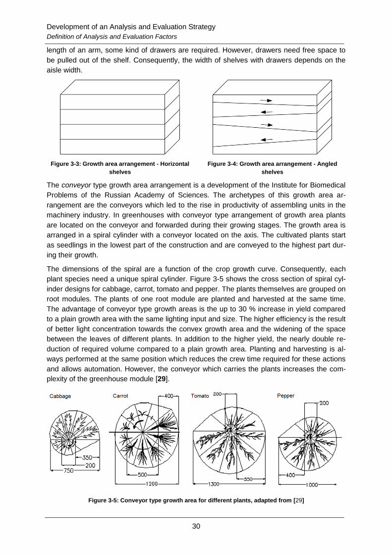
Development of an Analysis and Evaluation Strategy
Definition of Analysis and Evaluation Factors
30
length of an arm, some kind of drawers are required. However, drawers need free space to
be pulled out of the shelf. Consequently, the width of shelves with drawers depends on the
aisle width.
Figure 3-3: Growth area arrangement - Horizontal
shelves
Figure 3-4: Growth area arrangement - Angled
shelves
The conveyor type growth area arrangement is a development of the Institute for Biomedical
Problems of the Russian Academy of Sciences. The archetypes of this growth area ar-
rangement are the conveyors which led to the rise in productivity of assembling units in the
machinery industry. In greenhouses with conveyor type arrangement of growth area plants
are located on the conveyor and forwarded during their growing stages. The growth area is
arranged in a spiral cylinder with a conveyor located on the axis. The cultivated plants start
as seedlings in the lowest part of the construction and are conveyed to the highest part dur-
ing their growth.
The dimensions of the spiral are a function of the crop growth curve. Consequently, each
plant species need a unique spiral cylinder. Figure 3-5 shows the cross section of spiral cyl-
inder designs for cabbage, carrot, tomato and pepper. The plants themselves are grouped on
root modules. The plants of one root module are planted and harvested at the same time.
The advantage of conveyor type growth areas is the up to 30 % increase in yield compared
to a plain growth area with the same lighting input and size. The higher efficiency is the result
of better light concentration towards the convex growth area and the widening of the space
between the leaves of different plants. In addition to the higher yield, the nearly double re-
duction of required volume compared to a plain growth area. Planting and harvesting is al-
ways performed at the same position which reduces the crew time required for these actions
and allows automation. However, the conveyor which carries the plants increases the com-
plexity of the greenhouse module [29].
Figure 3-5: Conveyor type growth area for different plants, adapted from [29]
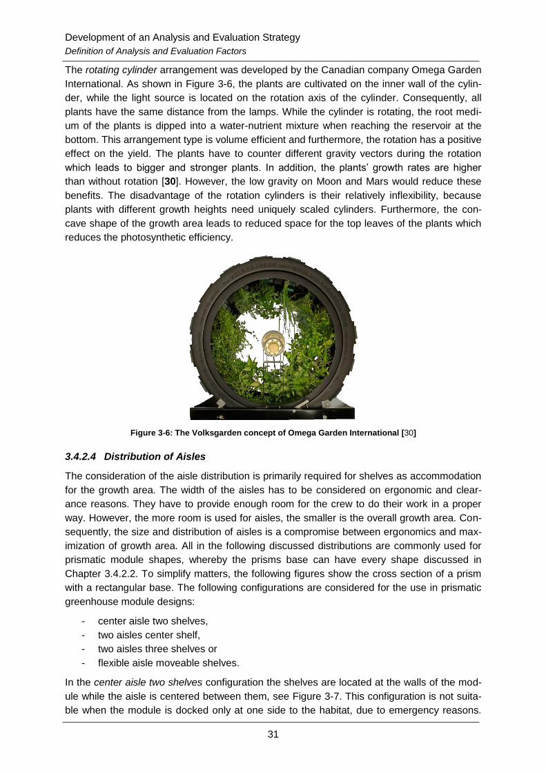
Development of an Analysis and Evaluation Strategy
Definition of Analysis and Evaluation Factors
31
The rotating cylinder arrangement was developed by the Canadian company Omega Garden
International. As shown in Figure 3-6, the plants are cultivated on the inner wall of the cylin-
der, while the light source is located on the rotation axis of the cylinder. Consequently, all
plants have the same distance from the lamps. While the cylinder is rotating, the root medi-
um of the plants is dipped into a water-nutrient mixture when reaching the reservoir at the
bottom. This arrangement type is volume efficient and furthermore, the rotation has a positive
effect on the yield. The plants have to counter different gravity vectors during the rotation
which leads to bigger and stronger plants. In addition, the plants’ growth rates are higher
than without rotation [30]. However, the low gravity on Moon and Mars would reduce these
benefits. The disadvantage of the rotation cylinders is their relatively inflexibility, because
plants with different growth heights need uniquely scaled cylinders. Furthermore, the con-
cave shape of the growth area leads to reduced space for the top leaves of the plants which
reduces the photosynthetic efficiency.
Figure 3-6: The Volksgarden concept of Omega Garden International [30]
3.4.2.4 Distribution of Aisles
The consideration of the aisle distribution is primarily required for shelves as accommodation
for the growth area. The width of the aisles has to be considered on ergonomic and clear-
ance reasons. They have to provide enough room for the crew to do their work in a proper
way. However, the more room is used for aisles, the smaller is the overall growth area. Con-
sequently, the size and distribution of aisles is a compromise between ergonomics and max-
imization of growth area. All in the following discussed distributions are commonly used for
prismatic module shapes, whereby the prisms base can have every shape discussed in
Chapter 3.4.2.2. To simplify matters, the following figures show the cross section of a prism
with a rectangular base. The following configurations are considered for the use in prismatic
greenhouse module designs:
- center aisle two shelves,
- two aisles center shelf,
- two aisles three shelves or
- flexible aisle moveable shelves.
In the center aisle two shelves configuration the shelves are located at the walls of the mod-
ule while the aisle is centered between them, see Figure 3-7. This configuration is not suita-
ble when the module is docked only at one side to the habitat, due to emergency reasons.
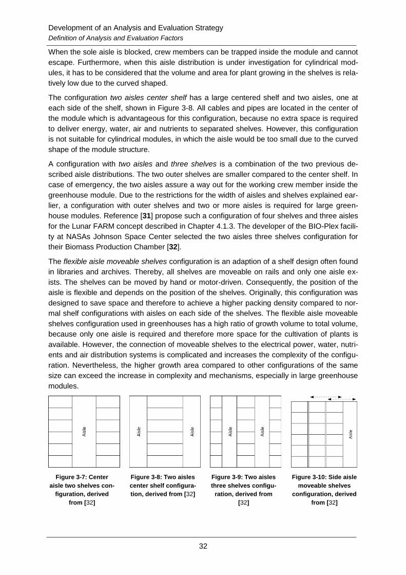
Development of an Analysis and Evaluation Strategy
Definition of Analysis and Evaluation Factors
32
When the sole aisle is blocked, crew members can be trapped inside the module and cannot
escape. Furthermore, when this aisle distribution is under investigation for cylindrical mod-
ules, it has to be considered that the volume and area for plant growing in the shelves is rela-
tively low due to the curved shaped.
The configuration two aisles center shelf has a large centered shelf and two aisles, one at
each side of the shelf, shown in Figure 3-8. All cables and pipes are located in the center of
the module which is advantageous for this configuration, because no extra space is required
to deliver energy, water, air and nutrients to separated shelves. However, this configuration
is not suitable for cylindrical modules, in which the aisle would be too small due to the curved
shape of the module structure.
A configuration with two aisles and three shelves is a combination of the two previous de-
scribed aisle distributions. The two outer shelves are smaller compared to the center shelf. In
case of emergency, the two aisles assure a way out for the working crew member inside the
greenhouse module. Due to the restrictions for the width of aisles and shelves explained ear-
lier, a configuration with outer shelves and two or more aisles is required for large green-
house modules. Reference [31] propose such a configuration of four shelves and three aisles
for the Lunar FARM concept described in Chapter 4.1.3. The developer of the BIO-Plex facili-
ty at NASAs Johnson Space Center selected the two aisles three shelves configuration for
their Biomass Production Chamber [32].
The flexible aisle moveable shelves configuration is an adaption of a shelf design often found
in libraries and archives. Thereby, all shelves are moveable on rails and only one aisle ex-
ists. The shelves can be moved by hand or motor-driven. Consequently, the position of the
aisle is flexible and depends on the position of the shelves. Originally, this configuration was
designed to save space and therefore to achieve a higher packing density compared to nor-
mal shelf configurations with aisles on each side of the shelves. The flexible aisle moveable
shelves configuration used in greenhouses has a high ratio of growth volume to total volume,
because only one aisle is required and therefore more space for the cultivation of plants is
available. However, the connection of moveable shelves to the electrical power, water, nutri-
ents and air distribution systems is complicated and increases the complexity of the configu-
ration. Nevertheless, the higher growth area compared to other configurations of the same
size can exceed the increase in complexity and mechanisms, especially in large greenhouse
modules.
Figure 3-7: Center
aisle two shelves con-
figuration, derived
from [32]
Figure 3-8: Two aisles
center shelf configura-
tion, derived from [32]
Figure 3-9: Two aisles
three shelves configu-
ration, derived from
[32]
Figure 3-10: Side aisle
moveable shelves
configuration, derived
from [32]

Development of an Analysis and Evaluation Strategy
Definition of Analysis and Evaluation Factors
33
3.4.2.5 Module Structure
The module structure affects several other parameters, but mainly the mass and complexity.
Table 3-10 shows the estimated total mass of different types of module structure for an inter-
nal volume of 655 m3. The structure of greenhouse modules can be:
- rigid,
- semi-deployable,
- fully deployable or
- made out of in situ materials.
Rigid structural designs are the common way for the construction of crewed modules. Ac-
cording to reference [31], the advantages of rigid structures are the confidence in the tech-
nology and the pre-installation and verification of all equipment before launch. In addition a
first set of plants can be planted and grown during the transfer to assure a continuous har-
vesting cycle from the arrival at the destination. However, rigid structures have to be strong
enough to withstand the loads during launch from Earth. Therefore, the mass of rigid struc-
tures is significantly higher than for other structural designs. Reference [31] estimates the
mass of a rigid greenhouse module with a length of 12 meters, a diameter of 8 meters and
an internal volume of 655 cubic meters to around 8000 kg. Furthermore, the dimensions of
rigid structures are defined by the fairings of available launch systems.
Semi-deployable or hybrid designs of greenhouses has a rigid structural compartment and
attached deployable sections. Hybrid designs combine the advantages of rigid and deploya-
ble structures with a moderate mass. The mass and volume of semi-deployable designs are
less than for rigid ones, while it is still possible to preinstall systems and plants. The deploy-
ing mechanisms increase the complexity. In addition, the interface between the rigid and the
deployable sections increase the complexity even more and are weak spots for leakages.
Consequently, the complexity of hybrid designs exceeds that of fully deployable systems.
However, a semi-deployable greenhouse module with dimensions of 12 meters length, 8 me-
ters diameter and an internal volume of 655 cubic meters would have a mass around 5500
kg [31].
Fully deployable or inflatable structures are currently under investigation by all space agen-
cies and some companies. Modules with deployable structures usually are packed to a rela-
tively small volume and unfolded at the target location, which reduces the mass of the mod-
ule, but increases the complexity due to the required deploying mechanisms. Reference [31]
estimates the mass of a fully deployable greenhouse module with a length of 14 meters, a
diameter of 8 meters and an internal volume of 655 cubic meters to around 1200 kg. Inflata-
ble structures usually have a shell out of Kevlar combined with other elastic polymeric mate-
rials. The materials make the shell flexible, light weight and strong enough to withstand the
environmental conditions [31]. In fully deployable modules plants cannot be planted until the
structure is completely enfolded, which is disadvantageous, because deployable greenhous-
es need a setup time before the first plants can be harvested. The nutrition of the crew for
this timespan has to be covered with stored food.
Development of an Analysis and Evaluation Strategy
Definition of Analysis and Evaluation Factors
34
Table 3-10: Estimated mass for different structural types for a volume of 655 m3, derived from [31]
Rigid 8000 kg
Semi-deployable 5500 kg
Deployable 1200 kg
The usage of in situ materials is also possible to build greenhouse modules on other plane-
tary bodies. Thereby, the materials can be applied on pre-fabricated structures to shield the
crew against radiation or the materials are used to create construction components for the
greenhouse. In addition, the local terrain, like caves, tunnels, lava tubes, mountains and cra-
ters himself can be used as structures. Therefore, a pressurized environment is created by
sealing the existing terrain formations against the environment to provide a suitable atmos-
phere for plants and humans. Module structures which use or are out of in situ materials
would reduce the launch mass of greenhouse modules significantly. Consequently, the costs
for these modules are lower than for pre-fabricated modules. However, further research in
the usage of in situ materials is required before greenhouse modules build out of them are
feasible [28].
3.4.2.6 Adaptability of Internal Configuration
The internal configuration has to support the plants during all growth stages. To maximize
the yield of the cultivated plants, the internal configuration has to be adapted while the plant
is growing. Furthermore, it is essential that the configuration is somehow adaptable to differ-
ent plant species. Especially, the adaptableness of the growth height is necessary to assure
a customizable internal configuration. The internal configuration of greenhouses can be clas-
sified as:
- inflexible,
- semi-flexible or
- flexible.
Inflexible internal configuration cannot be adapted once they are assembled. Consequently,
the grow height is given through the design of the greenhouse’s internal configuration. This
type of internal configuration does not increase the complexity of the module, but the achiev-
able yield is lower compared to semi-flexible and flexible configurations.
In semi-flexible designs the crew can adjust some parameters of the internal configuration
during the mission to change the plant configuration. Furthermore, semi-flexible designs pro-
vide some options to react on unscheduled events. Depending on the mechanisms used for
the adaptableness, the complexity of the greenhouse module can increase.
Flexible internal configurations are fully adaptable to a broad spectrum of parameter settings,
which increases the amount of required mechanisms and systems significantly. However, the
increase in yield and the ability to change the plant configuration in every way can legitimate
the higher complexity of the greenhouse module.
Development of an Analysis and Evaluation Strategy
Definition of Analysis and Evaluation Factors
35
3.4.2.7 Level of Automation
Automation of processes inside greenhouse modules is important to reduce the crew time
required to plant, cultivate and harvest plants. Crew time is valuable during space missions,
see Chapter 3.4.5.10, and all systems which can reduce the work load of the crew have to be
investigated on their applicability [33]. Nevertheless, a higher level of automation would in-
crease the complexity of greenhouse modules. Furthermore, the direct interaction with plants
can satisfy psychological needs of the crew, see Chapter 3.4.5.11., subsequently the level of
automation of greenhouse modules has to be considered wisely.
Depending on the integrated systems, greenhouse modules can have:
- none,
- partial or
- full
automation.
In greenhouses without any automation processes like planting, harvesting, nutrient mixing,
and monitoring are performed by crew members, which generates high work load. The com-
plexity of greenhouse modules without any automation systems would be very low compared
to the other types of automation. However, such greenhouse modules are not suitable for
planetary habitats, in which the crew size and consequently the available work power are re-
stricted.
Partial automation is common in today’s greenhouse module concepts. Thereby, some tasks
are fulfilled by computers and control algorithms. The automatically control of temperature,
lighting, humidity, ventilation, nutrient mixture and water supply is well known and was tested
in several terrestrial testbeds. A partial automation should be the least level of automation for
greenhouse modules proposed for future planetary habitats.
Fully automated greenhouse modules cover all tasks required to maintain the food produc-
tion at the predicted level. Besides the monitoring and controlling of environmental and met-
abolic conditions, fully automated greenhouses have the ability to plant and harvest the culti-
vated plants without the help of crewmembers. Consequently, the work load on the crew is
limited to monitoring and programming the automation processes. However, greenhouse
modules with full automation have a high complexity compared to the other two types.
3.4.2.8 Module Mass, Dimensions and Volumes
The module mass directly affects the costs of greenhouse modules. Especially, the launch
and transfer costs depend on the mass of the modules. The heavier the module, the higher
are the costs. Furthermore, the overall mass per module should not exceed the launch ca-
pacity of available launch systems. The proposed unit for the module mass is kilogram, kg.
The module dimensions are required for the calculation of overall and pressurized volume.
Typical dimensions are length, height, width and diameter. Dimensions are commonly meas-
ured in meter, m.
For the analysis of the volume of greenhouse modules total volume, pressurized volume and
the ratio of growth volume per total volume have to be considered. The total volume is calcu-
lated by the outer dimensions of the module and is mainly required for the selection of the
launch system and fairing. The pressurized volume is any volume that contains an atmos-

Development of an Analysis and Evaluation Strategy
Definition of Analysis and Evaluation Factors
36
pheric pressure suitable for humans and/or plants. The factor specific cultivation volume is
established to evaluate the efficient use of volume. Growth volume is the volume which can
be used for plant cultivation. It is calculated by the multiplication of the growth area in square
meters with the appropriate maximum growth height in meters. The higher the ratio of cultiva-
tion volume per total volume, the higher is the efficient use of volume. All volumes are re-
ported in cubic meters, m3.
3.4.2.9 Complexity
The complexity of greenhouse modules depends on the number of different elements, on the
amount of interconnections between the elements, on the functionality of the interconnec-
tions, and on the time dependency of the elements. The more elements are implemented in
the greenhouse, the more interconnections are between these elements. Furthermore, the
higher the time dependency of these elements, the higher is the complexity of the green-
house module.
A highly complex system has a greater potential for failures compared to systems with a low-
er complexity. However, a higher complexity often results in reduced work load for the crew
and in higher yields. Therefore, the performance of greenhouse modules with a high level of
complexity can exceed those of low complexity and can be applicable for the use in planetary
habitats. Nevertheless, the complexity of systems cannot be measured as a pure value.
Consequently, the analysis of a greenhouses complexity is generally subjective. During this
thesis the complexity of greenhouse concepts is evaluated by comparing the concepts to
each other.
3.4.3 Environmental Factors
3.4.3.1 Definition
The defined set of environmental factors encompasses all analysis and evaluation factors
related to the environmental control subsystems described in Chapter 2.5. Therefore, the en-
vironmental factors concern the atmosphere control subsystem, the water control subsystem,
the lighting control subsystem and the thermal control subsystem. There were ten environ-
mental factors identified during this thesis, five qualitative and five quantitative. The Air Con-
trol Subsystem (ACS) is analyzed and evaluated with the factors atmospheric composition,
trace gas treatment, humidity, atmospheric pressure and the concentrations of carbon diox-
ide and oxygen. There are no environmental factors defined for the analysis of the Water
Control Subsystem (WCS) during this thesis, because the design of this system is nearly the
same in every greenhouse module. However, some factors related to the WCS are part of
the interface factors category, because they describe the interface of the WCS with the habi-
tat. For the evaluation of the Lighting Control Subsystem (LCS) the factors lighting type, light-
ing strategy and photosynthetic period are established. The type of temperature control and
the air temperature are used to analyze and evaluate the TCS of greenhouse modules. Table
3-11 shows a summary of all environmental factors split into two columns, one for qualitative
factors and one for quantitative factors.
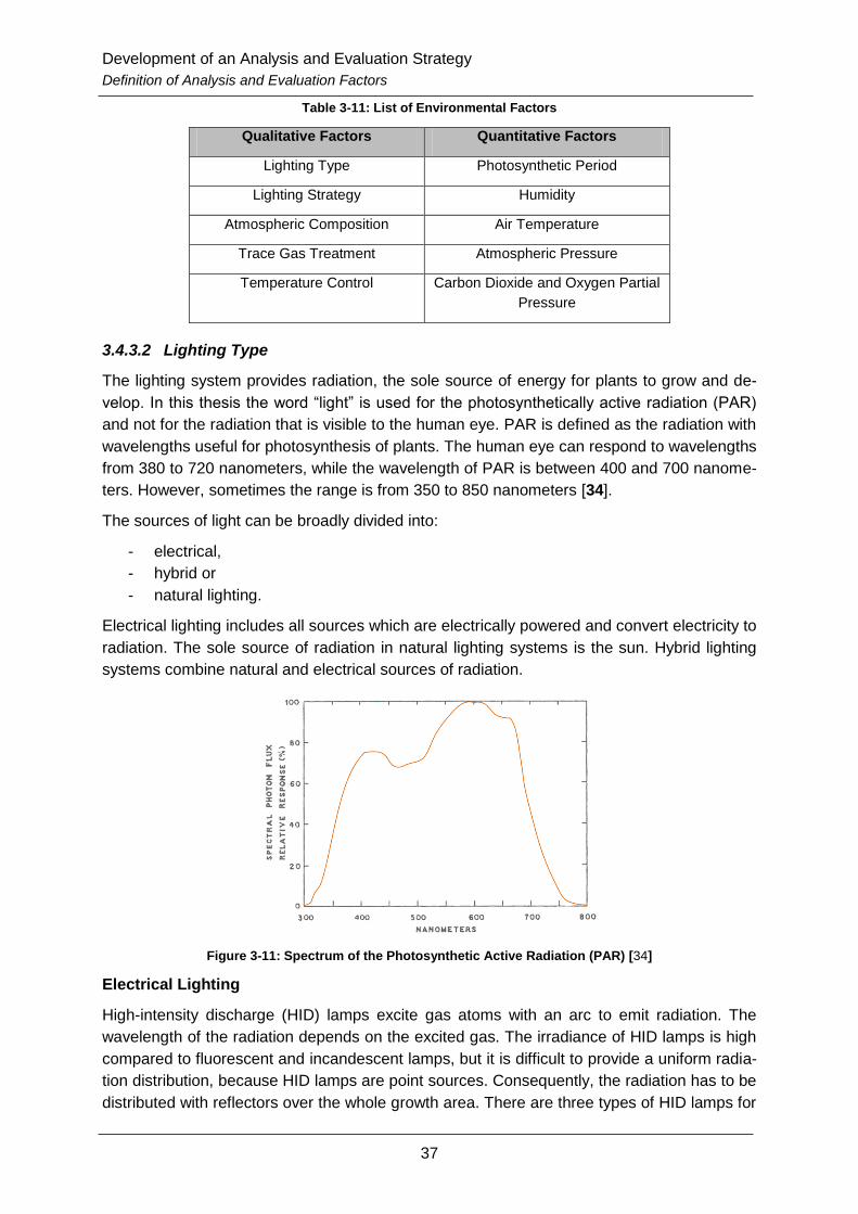
Development of an Analysis and Evaluation Strategy
Definition of Analysis and Evaluation Factors
37
Table 3-11: List of Environmental Factors
Qualitative Factors Quantitative Factors
Lighting Type Photosynthetic Period
Lighting Strategy Humidity
Atmospheric Composition Air Temperature
Trace Gas Treatment Atmospheric Pressure
Temperature Control Carbon Dioxide and Oxygen Partial
Pressure
3.4.3.2 Lighting Type
The lighting system provides radiation, the sole source of energy for plants to grow and de-
velop. In this thesis the word “light” is used for the photosynthetically active radiation (PAR)
and not for the radiation that is visible to the human eye. PAR is defined as the radiation with
wavelengths useful for photosynthesis of plants. The human eye can respond to wavelengths
from 380 to 720 nanometers, while the wavelength of PAR is between 400 and 700 nanome-
ters. However, sometimes the range is from 350 to 850 nanometers [34].
The sources of light can be broadly divided into:
- electrical,
- hybrid or
- natural lighting.
Electrical lighting includes all sources which are electrically powered and convert electricity to
radiation. The sole source of radiation in natural lighting systems is the sun. Hybrid lighting
systems combine natural and electrical sources of radiation.
Figure 3-11: Spectrum of the Photosynthetic Active Radiation (PAR) [34]
Electrical Lighting
High-intensity discharge (HID) lamps excite gas atoms with an arc to emit radiation. The
wavelength of the radiation depends on the excited gas. The irradiance of HID lamps is high
compared to fluorescent and incandescent lamps, but it is difficult to provide a uniform radia-
tion distribution, because HID lamps are point sources. Consequently, the radiation has to be
distributed with reflectors over the whole growth area. There are three types of HID lamps for
Development of an Analysis and Evaluation Strategy
Definition of Analysis and Evaluation Factors
38
the provision of radiation to plants: high-pressure sodium lamps, metal halide lamps and
mercury lamps [34].
High-pressure sodium (HPS) lamps produce radiation through exciting of highly concentrated
sodium vapor and a small amount of mercury with an electrically powered arc. The spectrum
of the emitted radiation is mainly between 550 and 650 nanometers, but low emission be-
tween 400 and 500 nanometers is also produced, see Figure 3-12. Hence, there is low emis-
sion in blue wavelengths. Therefore, lamps with higher irradiance in the blue spectrum have
to be added to the lighting systems to provide this spectrum to the plants. HPS lamps have a
high PAR efficiency compared to fluorescent, incandescence and other HID lamps. In addi-
tion, the lifetime of HPS lamps is high and their intensity is reduced slowly as the lamp ages
[34].
Metal halide (MH) lamps excite vapors of metal halides (iodides of thorium, thallium, of sodi-
um) and small portions of mercury to produce radiation. The wavelengths of the emitted pho-
tons depend on the gas inside the tube of the MH lamps. The main radiation output of MH
lamps is between 400 and 700 nanometers. The spectrum of a MH lamp compared to PAR is
shown in Figure 3-13. The disadvantages of MH lamps are the differences in spectral distri-
bution of different lamps and the spectral shift when the lamps age. The PAR efficiency of
MH lamps is slightly lower than that of HPS lamps. The average lifetime of MH lamps ranges
from 12000 hours for 1000 W lamps to 20000 hours for 400 W lamps. The intensity of MH
lamps decreases rapidly over time. After half of the lifetime the intensity is only 75 % of new
lamps [34].
In mercury lamps vapor of mercury is excited by an electrical arc. The emitted photons have
a bluish spectrum. Mercury lamps have a long average lifetime of 24000 hours, but after half
of the lifetime, the output is only 70 to 85 % compared to new lamps. The biggest disad-
vantage of mercury lamps is the significantly low PAR efficiency. Unless UV or blue wave-
lengths are required, mercury lamps are less recommended for the lighting of plants [34].
Fluorescent lamps are long glass tubes filled with mercury vapor under low pressure and an
inert gas, usually argon. At each end of the glass tube is an electrode. When a proper volt-
age is applied on the electrodes, an electric arc between them is generated. The arc excites
the mercury ions and when they fall back to the ground state, radiation mainly at a wave-
length of 253.7 nanometers is emitted. Photons with this wavelength are not suitable for
plants. Therefore, the inner wall of the glass tube is coated with fluorescent powder, usually
phosphor. The phosphor is activated by the incoming photons and emits new photons pri-
marily at longer wavelengths suitable for plant growing. The spectrum of fluorescent lamps
depends on the used phosphor mixture for the coating; the spectrum of a cool white fluores-
cent lamp is shown in Figure 3-14. Fluorescent lamps provide a continuous and uniformly
distributed radiation when placed closed together. The PAR efficiency of fluorescent lamps is
generally high, but is affected by the ambient temperature. The maximum output of fluores-
cent lamps is at a temperature of 38°C. Therefore, the ambient temperature has to be slightly
below 38°C to provide the maximum output. However, the low operating temperature reduc-
es the heat input into the growing area. During the operation the coating of the electrodes is
evaporated, mainly during the start-up. Consequently, the frequency of turning the lamps on
and off affects the lifetime. During the first 100 hours of operation, the output of fluorescent
lamps decreases rapidly. After this period the degradation is more continuous, leading to 70
% or less after 6000 hours [34].
Development of an Analysis and Evaluation Strategy
Definition of Analysis and Evaluation Factors
39
Incandescent Lamps utilize heated bodies to emit light. The light of incandescent lamps is
blackbody radiation. Consequently, the wavelengths of the photons depend on the tempera-
ture of the heated element. To create light useable by plants a temperature above 2600°K is
required. In commercial incandescent lamps filaments made of tungsten are heated with
electricity to a temperature between 2770 and 3050°K. The higher the voltage, the higher the
temperature raises. The spectrum of the emitted photons has a large component of wave-
lengths in the infrared spectral band. Figure 3-15 shows the comparison of the spectrum of
an incandescent lamp and PAR. Hence, most of the electrical energy used by incandescent
lamps is converted to heat, therefore, the efficiency of these lamps is low and not competitive
to over lamp types. In addition, the heat generated by of incandescent lamps has to be re-
moved out of the growth area to avoid damaging of the plants. The lifetime of commercially
available incandescent lamps ranges from 700 to 1000 hours and the output at the end of life
is about 85 % of the original. The very low lifetime and efficiency compared to other lamp
types leads to the conclusion that incandescent lamps are not recommended for the use in
lighting systems [34].
Low-pressure sodium (LPS) lamps are similar to HPS lamps. Contrary to HPS lamps, the
pressure in LPS lamps is lower and no mercury vapor is present. Thus, only the excited so-
dium provides the radiation output of LPS lamps. The spectrum of the radiation is limited to
wavelengths around 589 nanometers, see Figure 3-16. The output of LPS lamps is not high
enough to provide sufficient lighting for plants. Therefore, LPS lamps are not recommended
as radiation sources for plant growing [34].
Xenon lamps are able to most nearly duplicate the solar spectrum and irradiance. However,
xenon lamps are expensive and generate ozone, which is toxic to plants and humans. The
spectrum of the emitted photons has large quantities of infrared radiation. Infrared radiation
cannot be used by plants and increases the cooling requirements for the growth area. Con-
sequently, xenon lamps have only limited use in experimental growth chambers and are not
recommended for the use in high productive greenhouses [34].
Sulfur Lamps, also known as microwave-powered lamps, are electrodeless lighting devices.
Generally, a sulfur lamp consists of a quartz bulb filled with sulfur vapor and small amounts
of argon vapor. The vapor is excited by microwaves generated by a magnetron. The excita-
tion of the atoms results in an emission of photons [35]. The spectrum of sulfur lamps is
comparable to the suns. However, the intensity of the infrared band is lower for sulfur lamps.
The spectrum of a sulfur lamp compared to PAR is shown in Figure 3-17. Consequently, the
heat production of microwave-powered sulfur lamps is low. The advantages of sulfur lamps
are their small size and their nearly sun-like spectrum. The efficiency for the conversion of
electrical energy to radiation is higher than for HPS lamps, but due to the low efficiency of the
magnetron the overall efficiency is lower than that of HPS lamps. The average lifetime of sul-
fur lamps is around 20000 and the degradation of the radiation output is relatively low, lead-
ing to 90 % of the original value [34].
Light-emitting diodes (LED) are semiconductor devices which convert electricity to radiation.
There are three types of LEDs suitable as radiation sources for plants: discrete LEDs, print-
ed-circuit LEDs, and phosphor-based LEDs. LEDs are a comparatively new technology. The
efficiency, lifetime and output are still increasing, while the costs are decreasing through the
raising demands. The small size, high efficiency and long lifetime compared to other lighting
sources make them very interesting for the usage in plant growing systems. Unlike other

Development of an Analysis and Evaluation Strategy
Definition of Analysis and Evaluation Factors
40
lamp types, the light output of LEDs is current controlled. Hence, the brightness directly af-
fects the required power consumption [34].
Discrete LEDs emit photons with wavelengths in a narrow spectrum, depending on the con-
struction material. Usually, the spectral band is only 50 to 100 nanometers wide. Conse-
quently, LEDs with different colors are required to provide the light spectrum that plants
need. In past studies red, yellow-green and blue LEDs were used in combination. For the
spectrum from blue to green (460 - 550 nm) indium gallium nitride (InGaN) and for the spec-
trum from yellow to red (560 – 630 nm) aluminum gallium indium phosphide (AlGaInP) is
used as the base material. Figure 3-18 shows the spectrum of a blue, a yellow and a red dis-
crete LED compared to PAR. According to reference [36], commercially available LEDs with
more than 20 % efficiency are available and efficiencies over 50 % are expected in the next
decade.
The printed-circuit LEDs are small and applied on wafers in large numbers. This type of LED
has no plastic lenses like discrete LEDs. The package density of printed-circuit LEDs is high,
reaching up to 132 LEDs in an area of 6.25 cm2. This technique provides bright light levels.
Furthermore, each LED can be fabricated out of different materials, and therefore, different
colors are feasible. Consequently, the color mixture of printed-circuit LED arrays can be
adapted to the spectral needs of plants. However, it is not possible to replace a single broken
LED. To repair a printed-circuit LED, the whole array has to be replaced by a new one [37].
Phosphor-based LEDs, also known as white LEDs, are the combination of the common LED
technology with the technique of fluorescent lamps. Usually, a single blue LED made of galli-
um nitride (GaN) is used together with different mixtures of phosphor to generate a uniform,
sun-like white light. Therefore, the inner side of the bulb of a bluish LED is coated with a
phosphor mixture. The phosphor starts to emit a broad spectrum of light when hit by the pho-
tons generated by the LED. The broad spectrum from 500 to 700 nanometers could make
this type of LEDs suitable for plant growing. However, this technology is currently under de-
velopment to replace the commonly used incandescent lamps in household. Consequently,
progress in the commercialization of the technique is expected in the near future [36].

Development of an Analysis and Evaluation Strategy
Definition of Analysis and Evaluation Factors
41
Figure 3-12: HPS lamp spectrum compared to PAR
(orange line) [34]
Figure 3-13: MH lamp spectrum compared to PAR
(orange line), derived from [38]
Figure 3-14: Fluorescent lamp spectrum compared
to PAR (orange line) [34]
Figure 3-15: Incandescent lamp spectrum com-
pared to PAR (orange line) [34]
Figure 3-16: LPS lamp spectrum compared to PAR
(orange line) [34]
Figure 3-17: Sulfur lamp spectrum compared to
PAR (orange line), derived from [38]
Figure 3-18: Spectrum of blue, yellow, red discrete LEDs compared to PAR (orange line) [34]

Development of an Analysis and Evaluation Strategy
Definition of Analysis and Evaluation Factors
42
Natural Lighting
The utilization of sunlight is the basic form for providing plants radiation. All plants originated
on Earth are adapted to use the energy provided by the Sun’s radiation. Greenhouses with
natural lighting systems are established all over the world to grow food in a controlled envi-
ronment. Furthermore, natural lighting systems have the lowest power demands, compared
to electrical and hybrid lighting. Hence, the use of sunlight for growing plants in space and on
other planetary bodies looks promising. There are two ways of using the sun as radiation
source: direct natural lighting and indirect natural lighting.
In direct natural lighting systems the sunlight passes windows or transparent walls to reach
the growth area. Comparable to electrical lighting systems, direct natural lighting systems
need a powerful heat rejection system to reduce the heat generated by the infrared radiation
of the Sun. The environmental conditions of the nearest planetary bodies, Moon and the
Mars, complicate the use of direct natural lighting systems. One day on Moon is usually 28
Earth days long, hence there is 14 days sunlight followed by 14 days night. However, some
locations at the poles of Moon with nearly continuous sunlight exist. The day length on Mars
is similar to Earth, but the higher distance from the Sun lowers the average sunlight intensity
to 43 % of the terrestrial and due to the higher excentricity of the Martian orbit, the variation
of intensity is higher than on Earth. The inclination of Mars causes long seasonal periods,
which leads to long winter periods without sunlight at the poles. Other problems for the usage
of direct natural lighting on Mars are dust and dust storms. The wind on Mars is able to carry
dust over long distances and periodical strong and long lasting dust storms appear. The dust
covers the outside surfaces of windows and have to be removed to provide enough sunlight
for the plants. However, during dust storms the amount of sunlight reaching the surface of
Mars is too low for the demands of plants. Besides the problems with environmental condi-
tions at the location, the direct usage of sunlight can be more effective, and less mass and
cost intensive than electrical lighting [39].
Indirect natural lighting systems also utilize the energy of solar radiation to provide energy for
plant growth. They use reflectors, concentrators and plastic optic fibers to collect and distrib-
ute the sunlight over the whole growth area. Reflectors are polished surfaces or mirrors and
can be up to 95 % effective as direct sunlight systems, but contrary to those systems reflec-
tors reduce the heat input into the growth area and the heat can be directly rejected to the
environment without the need of additional radiators [39]. Concentrators usually consist of a
parabolic mirror and a collector. The mirror concentrates the incoming sunlight at the collec-
tor and the collector feeds fiber optic cables. These cables deliver the sunlight to the internal
lighting system inside the greenhouse and provide radiation for all plants. The power demand
for tracking the Sun is relatively low. The disadvantage of fiber optic cables is their low effi-
ciency. The longer the cables are, the lower is the efficiency. However, currently new tech-
nologies for fiber optic cables are under development and new optic cables with higher effi-
ciencies are expected in the near future. Besides the low heat input and low power demand
of indirect natural lighting systems are other advantages. Fiber optic cables can be easily re-
placed and therefore, it is possible to adjust the location of the light sources inside the
greenhouse. Furthermore, the cables can be used for intracanopy lighting which has ad-
vantages over other lighting distribution systems, see Chapter 3.4.3.3 [31].
Development of an Analysis and Evaluation Strategy
Definition of Analysis and Evaluation Factors
43
Hybrid Lighting
Hybrid lighting systems combine electrical and natural lighting. Both of these have their dis-
advantages, especially the high power demands of electrical lighting, which can be up to 45
% of the total power demand of a greenhouse [35], and the dependency on the sun of natural
lighting systems. Hybrid lighting systems can combine the benefits of both electrical and nat-
ural lighting to compensate their weaknesses. During sunshine the energy of the solar radia-
tion can be utilized for the plant growth, and to generate and store electrical energy. In night
periods the stored electrical energy is converted back to radiation for the plants by using an
electrical lighting system.
3.4.3.3 Lighting Strategy
The previous chapter described the different types of light sources and their advantages and
disadvantages. However, not only the lighting type, but also the lighting strategy affects the
plant growth and the efficiency of the lighting control subsystem. There are three options for
lamp positioning inside greenhouses:
- overhead lighting,
- sidewise lighting or
- intracanopy lighting.
Overhead lighting is the common strategy of positioning lamps. Thereby, the light sources
are attached to the ceiling of the greenhouse. The intensity of light decreases exponentially
when increasing the distance to the source. Therefore, the radiation source has to be close
to the leaves of plants to provide enough intensity while reducing the power demand. Due to
the plant growing, the distance between lamps and plants has to be adjusted to different
plant development stages to ensure a sufficient lighting and reducing the thermal loads to the
leaves. A problem of overhead lighting is shading of lower leaves by those above them,
which leads to net carbon loss via respiration and underdevelopment of plant parts. To re-
duce the effects of shading, the walls of greenhouse modules can be painted white or cov-
ered with polished surfaces to reflect the radiation and provide some light from the sides.
When reflectors are used, it has to be assured, that no spectral shift of the reflected light oc-
curs, because this can cause several problems concerning thermal and plant issues. But
even with reflective surfaces at the walls, shading cannot be totally avoided with overhead
lighting [34].
Sidewise describes a lighting strategy, where lamps are attached to the walls of the green-
house module. This lighting strategy requires a larger amount of space compared to over-
head lighting, but the power demand can be reduced by this type of lighting strategy. How-
ever, sidewise lighting also creates shading of plants that are further away from the walls and
therefore, the light distribution is suboptimal [37].
Intracanopy is the provision of lighting from the inside of the plant canopy. Thereby, the
lamps are located close to the leaves or even touching them. Consequently, this lighting
strategy is only applicable with low temperature light sources, which do not harm the plants.
Promising systems for intracanopy lighting are plastic optic fiber cables, LEDs, or light tubes.
Due to the close distance between leaves and lamps, the power demand of intracanopy is
lower compared to overhead and sidewise lighting. However, a lighting system with intracan-
opy lighting as a sole source of radiation would be complex. A combination of overhead and
Development of an Analysis and Evaluation Strategy
Definition of Analysis and Evaluation Factors
44
intracanopy lighting can increase the edible biomass, decrease the power demand and solve
problems with shading of leaves [37].
3.4.3.4 Atmospheric Composition
The atmospheric composition inside greenhouse modules affects the plant growth and the
humans’ ability to work. For plants the percentage of carbon dioxide in the air is an essential
factor for their welfare and growth. For humans a suitable amount of oxygen is required to
survive, as described in Chapter 2.2. Furthermore, the amount of carbon dioxide in the air is
also important for the health of the crew, who work in the greenhouse. There are three pos-
sible options of an atmospheric composition in greenhouses for space applications:
- local planetary atmosphere,
- an earth-like atmospheric composition or
- an atmosphere enriched with carbon dioxide.
The usage of a local planetary atmosphere in a greenhouse is a theoretical option. In our so-
lar system is no other known planetary body with an atmosphere suitable for plant growth.
However, some atmospheres contain elements that can be used in greenhouses. Especially
the carbon dioxide of the Martian atmosphere, see Chapter 2.1.2, could be extracted and in-
jected into the atmosphere of greenhouse modules to provide higher concentrations.
An earth-like atmosphere is the simplest way of an atmospheric composition inside green-
houses and provides enough carbon dioxide to sustain plant growth and enough oxygen to
allow humans to work without the need of respiratory protection devices. Every carbon diox-
ide concentration below the terrestrial concentration of 300 to 350 ppm decreases photosyn-
thesis and consequently, plant growth [40]. The advantage of an earth-like atmosphere is
that the atmosphere control system of the habitat can be used to maintain the atmosphere
inside the greenhouse. Furthermore, no airlocks are required to seal the atmosphere of the
greenhouse from that of the habitat.
Any atmospheric composition with a carbon dioxide level above the terrestrial is named an
atmosphere enriched with CO2. The responses of plants to elevated concentrations of carbon
dioxide depend on the plant species, developmental stage, irradiance, temperature, mineral
nutrition, and the size of the root zone. Table 3-12 shows a summary of the influences of a
CO2 enriched atmospheric composition on different processes of crop plants. The regulation
of the CO2 is quite difficult, because both plants and humans affect the CO2 in different ways.
The exhaled air of a working human contains 4 to 5 % carbon dioxide. Therefore, the amount
of CO2 in a sealed environment rises within in a few minutes to more than the tenfold of the
normal level. Plants consume CO2 to metabolize it in the photosynthetic process. Photosyn-
thesis requires energy in form of radiation. Consequently, the level of CO2 falls during lighting
periods. Without the energy of light, photosynthesis stop and the CO2 rises again due to res-
piration of plants up to twice as normal [40].
Development of an Analysis and Evaluation Strategy
Definition of Analysis and Evaluation Factors
45
Table 3-12: Responses of crop plants to an increase in CO2 concentration above earth-like atmosphere
[40]
Process Effects on Plants
Leaf photosynthetic rates Increase in all plants on first exposure. Little response above
1000 ppm and levels above 2000 ppm may be toxic.
Inhibition of photosynthesis by
source-sink imbalance
Response occurs in many species.
Leaf transpiration rate Decrease in all plants.
Leaf anatomical and biochemical
adaption
Leaf area, weight per unit area, thickness and number of mes-
ophyll cell layers increase in many species.
Canopy leaf area Usually increases.
Carbon partitioning among organs Proportion of carbon going to roots and stems is increased in
many, but not all, species.
Branching, flowering and fruiting Initiation and/or retention of these organs are increased in
many species.
Fruit and seed Increases in number and/or size of fruits and seeds.
Canopy water-use efficiency Increase in photosynthesis or yield contributes more than re-
duction in transpiration.
Yield Increases 32 % on average between 300 and 660 ppm for
plants in favorable conditions.
3.4.3.5 Trace Gas Treatment
Trace gases or air contaminants are an underestimated source of problems in closed envi-
ronment systems. Until today only little research is done in this field, because of the wide
spectrum of potential sources. The usual small air volume of closed environments emphasiz-
es the effects of trace gases, which are generally never or rarely seen in the terrestrial eco-
system. Air contaminants are sporadically produced by painting, cleaning or remodeling
structures and systems inside greenhouses. In addition to the sporadic production, the out-
gassing of some materials, mainly plastics, causes a constant source of toxic elements. Fur-
thermore, the ethylene exhaled by plants has to be treated. Table 3-13 shows a summary of
sources and effects of some toxic compounds identified during studies. Most of the ad-
dressed problems can be solved by choosing different, non-toxic materials or changing the
design of systems. There are three options of handling trace gases:
- neither monitoring nor treatment,
- monitoring of the amount of air contaminants or
- the combination of monitoring and separation of trace gases.
A greenhouse with neither monitoring nor separation of trace gases is no suitable option for a
controlled environment. The damage and symptoms caused at plants would be not repaira-
ble and could lead to diseases of the humans who ate the plants.
Monitoring of trace gases is the least option that has to be done in a closed environment. To
monitor the contaminants several portable and stationary measurement systems exist.
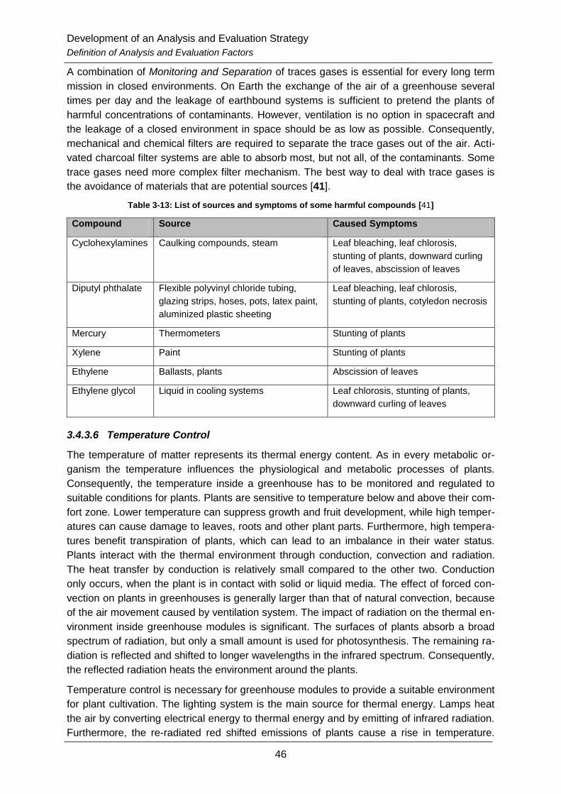
Development of an Analysis and Evaluation Strategy
Definition of Analysis and Evaluation Factors
46
A combination of Monitoring and Separation of traces gases is essential for every long term
mission in closed environments. On Earth the exchange of the air of a greenhouse several
times per day and the leakage of earthbound systems is sufficient to pretend the plants of
harmful concentrations of contaminants. However, ventilation is no option in spacecraft and
the leakage of a closed environment in space should be as low as possible. Consequently,
mechanical and chemical filters are required to separate the trace gases out of the air. Acti-
vated charcoal filter systems are able to absorb most, but not all, of the contaminants. Some
trace gases need more complex filter mechanism. The best way to deal with trace gases is
the avoidance of materials that are potential sources [41].
Table 3-13: List of sources and symptoms of some harmful compounds [41]
Compound Source Caused Symptoms
Cyclohexylamines Caulking compounds, steam Leaf bleaching, leaf chlorosis,
stunting of plants, downward curling
of leaves, abscission of leaves
Diputyl phthalate Flexible polyvinyl chloride tubing,
glazing strips, hoses, pots, latex paint,
aluminized plastic sheeting
Leaf bleaching, leaf chlorosis,
stunting of plants, cotyledon necrosis
Mercury Thermometers Stunting of plants
Xylene Paint Stunting of plants
Ethylene Ballasts, plants Abscission of leaves
Ethylene glycol Liquid in cooling systems Leaf chlorosis, stunting of plants,
downward curling of leaves
3.4.3.6 Temperature Control
The temperature of matter represents its thermal energy content. As in every metabolic or-
ganism the temperature influences the physiological and metabolic processes of plants.
Consequently, the temperature inside a greenhouse has to be monitored and regulated to
suitable conditions for plants. Plants are sensitive to temperature below and above their com-
fort zone. Lower temperature can suppress growth and fruit development, while high temper-
atures can cause damage to leaves, roots and other plant parts. Furthermore, high tempera-
tures benefit transpiration of plants, which can lead to an imbalance in their water status.
Plants interact with the thermal environment through conduction, convection and radiation.
The heat transfer by conduction is relatively small compared to the other two. Conduction
only occurs, when the plant is in contact with solid or liquid media. The effect of forced con-
vection on plants in greenhouses is generally larger than that of natural convection, because
of the air movement caused by ventilation system. The impact of radiation on the thermal en-
vironment inside greenhouse modules is significant. The surfaces of plants absorb a broad
spectrum of radiation, but only a small amount is used for photosynthesis. The remaining ra-
diation is reflected and shifted to longer wavelengths in the infrared spectrum. Consequently,
the reflected radiation heats the environment around the plants.
Temperature control is necessary for greenhouse modules to provide a suitable environment
for plant cultivation. The lighting system is the main source for thermal energy. Lamps heat
the air by converting electrical energy to thermal energy and by emitting of infrared radiation.
Furthermore, the re-radiated red shifted emissions of plants cause a rise in temperature.

Development of an Analysis and Evaluation Strategy
Definition of Analysis and Evaluation Factors
47
Consequently, the primary task of the thermal control subsystem during lighting periods is
cooling the inside of the greenhouse. Heat exchangers using chilled water or ethylene glycol
are the commonly used cooling system. During dark periods, heating units could be required
to maintain a warm enough air temperature. Therefore, electrical resistance heaters are
used. The temperature control system can be designed in three different ways:
- controlling the temperature of the whole greenhouse,
- temperature control for each plant species or
- temperature control per growth unit.
Control limited to the whole greenhouse is the simplest way to maintain the temperature. All
plants will be exposed to the same temperature. Therefore, the average temperature inside
the greenhouse would be a compromise between the requirements of all cultivated plants. In
this case the plants’ yield would be not the potential maximum.
A temperature control adapted to each plant species can maximize the biomass production
and yield. The complexity of such systems is higher than for control systems for the whole
greenhouse. More sensors, larger ventilation and cooling systems are required. Furthermore,
barriers between different plant species are necessary to maintain the temperature differ-
ence. Consequently, the masses of the thermal and air control subsystems are higher for the
temperature control of each plant species.
The monitoring and controlling of the temperature of each growth unit is challenging and re-
quires a complex system of sensors, pipes and fans. However, separate thermal controls for
each growth units can increase the yield due to specific temperatures. The increase in food
output has to be traded against the rise of complexity and mass of the system.
3.4.3.7 Photosynthetic Period
The photosynthetic period is another factor related to the lighting control subsystem. Besides
the provision of radiation with suitable wavelengths, see Chapter 3.4.3.2, the quantity of radi-
ation and the duration of the exposure to light affect the plant health and growth. The quantity
of radiation is named photosynthetic photon flux (PPF). The PPF is the amount of photons of
a specific wavelength that flow through an area in a defined timespan. The unit of PPF is mi-
cro moles per square meter per second for a specific waveband, μmol/(m2*s). The analysis of
the waveband is important to compare the PPF of different greenhouse concepts. Further-
more, it has to be investigated how long the PPF is applied to the plants.
The product of PPF and time is the quantity of energy delivered to the plants. As long as the
quantity of energy is constant, the growth rates of plants are similar. Consequently, continu-
ous exposure to light is possible to reduce the PPF and therefore, the energy required for
electrical lighting. When a continuous photosynthetic period is applied it has to considered,
that the temperature of the leaves can rise to a critical level. Usually, a day-night cycle of 16
hours light exposure and 8 hours darkness with a PPF of 400 to 500 μmol/(m2*s) for the
waveband of PAR leads to suitable growth rates. However, the PPF and duration of the pho-
tosynthetic period are plant specific and should be adjusted to every plant species to maxim-
ize the yield [34].
Development of an Analysis and Evaluation Strategy
Definition of Analysis and Evaluation Factors
48
3.4.3.8 Humidity
Humidity, also known as atmospheric water vapor, has several effects on the behavior of
plants. The energy balance of plants is indirectly affected by humidity. The direct effect of
humidity is the influence on the gas exchange between plants and their environment. Here-
by, the most significant impact of atmospheric water vapor is on transpiration: when humidity
decreases, transpiration increases. The plant water status is the balance of water gained by
roots and water evaporated over the surface of leaves. Low transpiration, as well as high,
can lead to an imbalance of the water status and therefore, can damage the plants or cause
sicknesses. High humidity stimulates the stomata of plants, small openings on the leaf which
can sense humidity and regulate the transpiration rate, to remain closed. Hence, the transpi-
ration and gas exchange is stopped, which leads to a reduced carbon dioxide intake reduced
photosynthesis and therefore, lower yields. Plants use transpiration to cool their body in a
same way humans do. Consequently, transpiration causes a heat transfer from plants to their
environment.
Humidity also affects the temperature control subsystem by increasing specific heat of the air
and due to the heat energy transfer caused by evaporation and condensation. The effects of
humidity on the chemical and biological environment of greenhouse modules are less signifi-
cant. A continuous measurement and control of humidity is challenging, but necessary. The
humidity control mechanisms are usually a combined task of air, water and temperature con-
trol subsystems. The usually small volume of closed environments leads to more extreme
levels of humidity, because the gas exchange with the outside is negligible. The control of
humidity has high energy demands due to the nature of energy required for evaporating and
condensation of water vapor. Condensation is used to reduce the humidity inside the green-
house. Therefore, surfaces with a temperature at or lower the dew point are required. The
condensed water has to be collected and removed out of the greenhouse. To higher the hu-
midity, water vapor is injected to the air.
Several definitions and units are known. For the analysis during this thesis the terms abso-
lute humidity and relative humidity are used. The absolute humidity is also known as water
vapor density or water vapor concentration and is the total amount of water inside a specific
volume of air. The unit is gram per cubic centimeter, g/cm3. The ratio of water vapor con-
tained in the air to that at saturation point at the same temperature is defined as relative hu-
midity and expressed as percentage. The usage of relative humidity for evaluation process is
problematic due to the dependency on the air temperature. However, relative humidity is a
commonly used value and as long as the temperature is also investigated, relative humidity
can be established as factor [42].
3.4.3.9 Air Temperature
The air temperature influences plants as described in Chapter 3.4.3.6. Therefore, an analysis
of the air temperature inside greenhouses of different concepts is essential. The temperature
has to be reported as average and range in degree Celsius, °C. Furthermore, the location of
the temperature is worth knowing, because temperature gradients between sections of the
greenhouse may exist.
Development of an Analysis and Evaluation Strategy
Definition of Analysis and Evaluation Factors
49
3.4.3.10 Atmospheric Pressure
The atmospheric pressure inside greenhouse modules affects the structural design, the leak
rate and the behavior of humans. According to references [43] and [44], the effects of the
atmospheric pressure on plants are negligible. However, the transpiration rate is slightly in-
creased in environments with an atmospheric pressure lower than the terrestrial average.
The design of pressurized modules for space applications is challenging, because the struc-
ture of spacecraft have to withstand the pressure difference between the inside of the mod-
ule and the ambient pressure at the location. Furthermore, the higher the pressure difference
between the inner and the outer of the module is, the higher the leakage rate. Low pressure
modules can be designed to reduce the structural loads and therefore, the mass of the mod-
ule [44]. In addition a reduced atmospheric pressure lowers the leakage rate. Consequently,
a low pressure environment inside greenhouse modules is applicable, as long as the human
requirements described in Chapter 2.2 and the demands of plants are met [45]. The atmos-
pheric pressure has to be reported in kilopascal, kPa.
3.4.3.11 Carbon Dioxide and Oxygen Partial Pressure
The CO2 partial pressure directly affects the yield and growth rates of plants, as described in
Chapter 3.4.3.4. Therefore, it is important to analyze the carbon dioxide level of the atmos-
phere inside greenhouse modules. The photosynthetic periods of plants lead to an oscillation
of the concentration. Consequently, the range and the average of the concentration have to
be investigated. Several units for gas concentrations exist, the most commonly used units
are the partial pressure and parts per million of volume. The proposed unit of this thesis is
the partial pressure in kilopascal, kPa [45].
The O2 partial pressure mainly influences the work ability of humans inside greenhouse
modules. The effects of different oxygen levels on humans are described in detail in Chapter
2.2. While humans need a sufficient partial pressure of oxygen, plants are able to grow with-
out O2. Furthermore, the efficiency of photosynthesis increases under lower concentrations
of oxygen [44]. Consequently, a compromise between the efficiency of plants and the work
ability of humans inside the greenhouse has to be considered. Options for reduced oxygen
levels are oxygen masks or hermetically closed suits for the crew working inside the green-
house, or fully automated greenhouses, which do not need human presence to growth and
harvest plants. Oxygen partial pressure is commonly reported in kilopascal, kPa [45].
3.4.4 Agricultural Factors
3.4.4.1 Definition
Agricultural factors refer to the tasks and requirements of the agricultural subsystem defined
in Chapter 2.5. Consequently, the established agricultural factors are used to analyze and
evaluate the plant cultivation subsystem, the nutrient delivery subsystem and the harvest &
cleaning subsystem. Nine agricultural factors are investigated, five qualitative and four quan-
titative factors. The Plant Cultivation Subsystem (PCS) is analyzed and evaluated on the
used growth medium, the installed plant monitoring system, the plant mixture, the planting
sequence, the cultivated plants, the biomass productivity, the specific growth area and the
grow height. The investigation of the nutrient supply is used for the analysis and evaluation of
the Nutrient Delivery Subsystem (NDS). For the Harvest & Cleaning Subsystem (HCS) no

Development of an Analysis and Evaluation Strategy
Definition of Analysis and Evaluation Factors
50
factors are defined, because the provided tools and stuff of this subsystem are independent
from the design of the greenhouse module. However, the size of the HCS is proportional to
the size of the greenhouse module. Table 3-14 shows a list of all agricultural factors split into
quantitative and qualitative factors.
Table 3-14: List of Agricultural Factors
Qualitative Factors Quantitative Agricultural Factors
Growth Medium Cultivated Plants
Plant Monitoring Biomass Productivity
Nutrient Supply Specific Growth Area
Plant Mixture Growth Height
Planting Sequence
3.4.4.2 Growth Medium
The growth media of greenhouse modules are the substances in which the roots of the culti-
vated plants reach and absorb the nutrients. The selection of an appropriate growth media
for greenhouse modules is challenging, because of several requirements an optimal growth
medium has to fulfill. Basically, the available growth media can be divided into the three cat-
egories:
- soil,
- soil-like or
- soilless.
Soil as growth medium can be either terrestrial or extraterrestrial soil. Soil-like growth media
are usually substrates, thereby, inert and organic substrates are considered. Soilless agricul-
ture methods are hydroponic and aeroponic. They do not use any kind of soil or substrates.
Soil
The growing of plants in terrestrial soil is the most commonly used cultivation method on
Earth. Soil agriculture is utilized by humans since several thousand years. Consequently, the
use of soil as grow medium in open fields and greenhouses is well understood. However,
terrestrial soil as growth medium for environmentally closed greenhouse modules in space is
not suitable. The launch and transportation costs for terrestrial soil are high compared to oth-
er growth media. According to reference [45], problems with microbiological contamination
are unpredictable and can cause a complete failure of the greenhouse module. Furthermore,
the handling of plants grown in soil during planting and harvesting under microgravity is diffi-
cult. Microgravity also inhibits drainage leading to water-logged soil, which can cause anaer-
obic reactions in the soil. Additionally, the absence of convection under microgravity prevents
aeration of the roots. Another problem with soil as growth medium is the potential absorption
of trace gases from the air, which could lead to problematic chemical reactions in the soil.
Since plants do not need terrestrial soil to grow as long as all required nutrients are provided,
terrestrial soil is not recommended for the use in space based greenhouse modules [45].
Extraterrestrial soil as growth medium shares the disadvantages of terrestrial soil, except the
transportation costs for the soil are absent. However, for the conversion of extraterrestrial
surface material to an appropriate growth medium requires special devise and systems.
Development of an Analysis and Evaluation Strategy
Definition of Analysis and Evaluation Factors
51
NASA undertakes research in the usage of lunar surface material, also known as regolith.
However, in its pure form, regolith is not suitable for growing plants, because it inhibits aera-
tion and water flow to the roots. Furthermore, regolith contains only small amounts of the re-
quired nutrients for plants and the potentially of toxicity of chromium and nickel in regolith is
not identified [46]. According to the references [46] and [47], growth media derived from local
planetary surface material look promising for the usage in greenhouse modules, but further
research is required to precisely determine their properties and growth conditions.
Soil-like
For inert substrates as growth medium commonly perlite, rockwool, polystyrenes and zeolites
are available. According to reference [46], zeolites are the most promising inert substrate for
greenhouse modules. Zeolites are crystalline, hydrated aluminosilicates containing loosey-
bound ions of potassium, sodium, calcium and magnesium. In nature about 50 zeolites exist
and several hundreds were developed by mankind in the last decades. The channels and
pores zeolites generally have, allow the storage of nutrient cations without changing the zeo-
lites themselves. Consequently, an inert substrate can act as a nutrient reservoir for plants.
Furthermore, zeolites are sterile to pathogenic microorganisms, which usually cause prob-
lems in soil based greenhouse modules [46]. Zeoponic agriculture is still under development
and further research is required to determine the benefits and disadvantages of this cultiva-
tion method. First experiments show the potential of zeoponics to overcome soil as growth
medium. However, zeolites share some disadvantages with soils [31]. The major disad-
vantage is the degradation of the zeolites over time, which results in a demand of new zeo-
lites after some growth periods. The new zeolites have to be delivered from Earth or pro-
duced in the habitat. Both options increase the resupply respectively launch mass of the
greenhouse module.
Organic substrates like straw or hay can be used as potential growth medium for extraterres-
trial greenhouses. However, organic substrates can react with the nutrient solution and will
decay over time, which increases the growth of pathogenic microorganisms inside the sub-
strate. Furthermore, the rotting of organic substrates creates trace gases and substances
which have to be treated and the decayed substrate has to be replaced with new one fre-
quently. Consequently, organic substrates are not recommended for the use in extraterrestri-
al greenhouse module, because of the unpredictable consequences of occurring bacteria,
fungi and other microorganisms.
Soilless
Hydroponic agriculture is a soilless cultivation method, because the roots of plants are hang
in an aerated, circulating liquid. The liquid mainly consists of water, enriched with nutrients
and oxygen. Reference [45] states, that hydroponic systems provide a precise control of nu-
trient composition, concentration, availability and pH. Hydroponic systems assure an appro-
priate of root zone oxygen and allow precise control of the root zone environment. Further-
more, low watering of plants cannot occur in these systems and it is not necessary to clean
the growth medium between crops, because there is no solid growth medium. The nutrient
delivery to the plants can be precisely controlled and maintained due to the concentration of
nutrients in the water flowing around the roots. Another advantage of hydroponic agriculture
is the possibility to recycle the used liquid nutrient solution, because it consists mainly of wa-
ter. Plants grown in hydroponic cultivation systems have a higher harvest index compared to
plants grown in soil. The harvest index is the ratio of edible biomass to inedible biomass of

Development of an Analysis and Evaluation Strategy
Definition of Analysis and Evaluation Factors
52
harvested plants. The higher harvest index results from a lower root mass of hydroponically
grown plants. Since nutrients and water are continually available in hydroponic systems,
plants need only small roots, which have only 3 to 4 % of the total dry weight, while the roots
of plants cultivated in soil generally have a dry weight of 30 to 40 %. However, the ad-
vantages of hydroponic agriculture bring significant disadvantages with them. Greenhouse
modules with hydroponic systems have a high system mass compared to other solutions,
even higher than soil based systems [45]. Furthermore, the large surfaces covered with wa-
ter can result in evaporation of water and consequently, increased humidity [42]. The transpi-
ration rate of plants grown in hydroponic systems is higher than in soil grown plants [48].
Nevertheless, hydroponic agriculture is a suitable cultivation method for greenhouse modules
in planetary habitats.
In aeroponic agriculture, the plants’ roots are not located in any form of substrate and are not
flowed around by water. They are hanging loosely in the air. Due to the absence of growth
medium, the system mass for an aeroponic greenhouse module is low compared to the other
cultivation methods. The nutrient solution is applied to the roots in the form of a fog created
by sprayers and injectors. Consequently, the required amount of nutrient solution is lower
than for other cultivation methods, because the nutrients are directly supplied to the roots
[45]. Aeroponic cultivation systems provide perfect aeration of the root zone which is im-
portant for an optimal root zone development and plant growth [31]. The nonexistence of a
growth medium leads to a negligible nutrient buffer capacity. Therefore, the nutrient solution
has to be applied on the roots in regular intervals to assure an optimal plant growth. Fur-
thermore, the nutrient composition and pH has to be controlled and adjusted frequently. The
root zone of an aeroponic cultivation system has to be confined to avoid the contact of nutri-
ent solution with the normal atmosphere of the greenhouse module [45]. The confinement of
the root zone is complicated, because the nutrient solution usually is moderately corrosive
and will damage any unprotected electronic and structural components. Furthermore, the nu-
trient solution can contain pathogenic microorganisms and the contact between them and
other plants and especially crew members have to be avoided at any cost. According to ref-
erence [45], aeroponic systems are not recommended for the use in extraterrestrial green-
house modules until the clogging of the sprayers and injectors can be eliminated, because
the cleaning of sprayers and the replacement of broken injectors is complicated and requires
too much crew time and spare parts.
3.4.4.3 Plant Monitoring
Plant monitoring is essential to maintain the optimum growth conditions of plants and to de-
tect diseases or abnormalities. Several plant monitoring systems and sensors exist to ob-
serve plants during their growth. Environmental sensor systems for temperature, humidity
and atmosphere composition can be used for indirect measurements of the plants’ welfare.
Fluorescent imaging systems can be used to observe the photosynthesis of plants. There-
fore, a single leaf of a plant is irradiated with a defined light spectrum. The spectrum of the
reflected radiation is measured and interpreted to achieve information about the photosyn-
thetic efficiency. The nutrient uptake of plants can be investigated by determining the con-
centration of nutrients in the nutrient solution. The dimensions of plant parts like leaves,
stems and blooms are measured manually or with the aid of laser imaging. Image sequences
of plants over a defined timespan can be analyzed by special designed software tools to de-
termine the growth rate. Furthermore, destructive investigation methods are available. These

Development of an Analysis and Evaluation Strategy
Definition of Analysis and Evaluation Factors
53
methods destroy a leaf or another plant part and analyze the residuals. However, destructive
methods are only suitable for research greenhouse modules. For food production green-
houses edible biomass is valuable and should not be destroyed as long as other investiga-
tion methods are feasible. The plant monitoring established during this thesis does not eval-
uate the applied sensor system of the analyzed concepts, but rather evaluates the level of
plant monitoring. The levels of plant monitoring:
- no plant monitoring,
- monitoring per plant species,
- per growth unit or
- per plant
are described in the following paragraphs.
No plant monitoring is only a theoretical option. Greenhouse modules without any plant moni-
toring are not suitable for space application, because the yield cannot be maximized. The
welfare of plants inside such greenhouse modules cannot be observed appropriately and
consequently, diseases and abnormalities can occur and lead to a complete failure.
Plant monitoring per plant species is the least option which should be established in green-
house modules. Thereby, the development and health of one plant per species is observed.
The analysis of this plant’s status then represents the average of all plants of this species.
This monitoring concept is inaccurate compared to the following to monitoring concepts.
However, plant monitoring per plant species is suitable for short duration missions and test
greenhouses.
Plant monitoring per growth unit is the optimal solution for extraterrestrial greenhouse mod-
ules which are usually subdivided into several growth units. A growth unit can contain only
one plant species or mixtures of species which have the same lighting and nutrient require-
ments. Monitoring systems for growth units measure all conditions inside the unit and ob-
serve the development of a selected plant to estimate the health status of all plants inside
this unit. Usually, each growth unit has its own sensor system for environmental parameter.
Investigations of plants’ physiology and welfare are undertaken by a mobile or robotic system
that is responsible for several growth units and examines each unit frequently. Plant monitor-
ing per growth unit is highly recommended for food production greenhouse modules, be-
cause this concept provides all required data for the maintenance of the module and maximi-
zation of the yield.
Monitoring of every plant requires more equipment than the other options and therefore, the
complexity of the monitoring system is high. Furthermore, the monitoring of every plant is not
necessary for the maintenance of greenhouse modules. In large greenhouse modules the
monitoring of every plant is impracticable due to the potentially high amount of plants. How-
ever, the monitoring of every plant can be valuable in test greenhouses, were the responses
of plants to different conditions is investigated.

Development of an Analysis and Evaluation Strategy
Definition of Analysis and Evaluation Factors
54
3.4.4.4 Nutrient Supply
The nutrient supply is part of the Nutrient Delivery System (NDS) as described in Chapter
2.5. This factor describes the way nutrients are provided to the NDS. In extraterrestrial
greenhouses the essential minerals for the plant growth has to be offered to the plants via
the NDS. The NDS itself is responsible for an adequate mixture of different nutrients. There-
fore, for each element of the mixture separate tanks exist. Usually, the nutrient mixture con-
sists of different nitrates and sulfates in combination with water. The nutrients themselves
can be provided as
- stored liquids and solids,
- by partial recycling or
- by full recycling of inedible biomass.
In stored nutrient concepts, nutrients are filled in tanks and taken from Earth with the launch
of the greenhouse module. The mission time of greenhouse modules is restricted to the
amount of nutrients contained in the tanks. For the extension of growth period, nutrients have
to be resupplied from Earth regularly. This type of nutrient supply is only suitable for small,
research or prototype greenhouse modules, because of the higher demand in required re-
supply mass compared to the other types.
Partial recycling concepts extract nutrients out of inedible biomass of harvested plants and
therefore, are able to produce some of the required nutrients. Nevertheless, partial recycling
systems cannot provide all required elements, because some of them are transferred to the
metabolism of the crew while eating the edible biomass of plants. However, this type of nutri-
ent provision reduces the resupply mass of nutrients and can provide up to 60 % of total in-
organic nutrient weight and 20 % of total organic carbon required by plants [45]. Consequent-
ly, partial recycling concepts are suitable for mid-sized greenhouse modules.
Full recycling nutrient supply systems gain the nutrients due to the recycling of all inedible
biomass produced by plants and all feces produced by crewmembers. This type of nutrient
supply is a nearly closed loop system, but leakages and imbalances in bio-chemical pro-
cesses prevent full closure. Nevertheless, a fully recycling concept requires only a very small
amount of resupply mass for nutrients compared to the other two types. Two reduce the re-
supply mass to zero the extraction of nutrients out of extraterrestrial soil has to be investigat-
ed. Consequently, a full recycling concept is suitable for greenhouse modules in large and
permanent extraterrestrial habitats and can reduce the dependency on resupply from Earth.
3.4.4.5 Plant Mixture
The plant mixture factor is established to analyze how plants of different species can be
grown together in greenhouse modules. In greenhouses plants are grown as
- monoculture or
- polyculture.
In greenhouse modules with monoculture, only one plant species is cultivated per growth
unit. This concept is the commonly used option for extraterrestrial greenhouse module con-
cepts. Plant growth is predictable and every plant species receives their perfect nutrient solu-
tions and optimal environmental conditions, because no compromise with other species has
to be made. However, monoculture can lead to inefficient growth area use, when the plant
Development of an Analysis and Evaluation Strategy
Definition of Analysis and Evaluation Factors
55
allocation is not planned appropriately. The lower complexity compared to polyculture rec-
ommends monoculture for the use in greenhouse modules for space applications.
Polycultural greenhouse modules cultivate different plant species together on the same
growth area. When the grown plants are selected carefully they can benefit from the pres-
ence of other plant species. However, polyculture is not suitable for every plant species and
is only recommended when the selected plant combinations are extensively tested over sev-
eral growth periods and generations and no incompatibilities are observed. Incompatibilities
between plant species can induce underdevelopment or even the death of plants. Usually,
most of the problems of polyculture occur in the root zone when the roots of one plant spe-
cies dispense substances which are toxic to the root system of the other plant species. Fur-
thermore, plants in a polyculture should have the same growth periods to assure seeding
and harvesting at the same time, which is necessary to prevent damaging of plants during
the processes. Consequently, polyculture can increase the biomass output per growth area,
but should only be established when the welfare of all plants can be guaranteed.
3.4.4.6 Planting Sequence
The planting sequence describes the way plants are settled into greenhouse modules and
directly affects the harvesting date of plants, assuming known growth durations. The se-
quence has to assure a continuous output of food and oxygen without or with only small fluc-
tuations. Two planting sequences are discussed for the implementation in greenhouse mod-
ules [49]:
- staggered planting or
- batch planting.
Staggered planting sequences, also known as conveyor planting, provide a nearly continu-
ous food and oxygen output, and carbon dioxide intake. This planting sequence is similar to
the just-in-time-production known from several industrial branches. A predefined amount of
plants of one species is seeded at the same time and consequently, harvested at the same
time. Thereby, the number of seeded plants depends on the amount of food needed at the
harvest date. Usually, staggered planting sequences do not produce surplus in food. Con-
sequently, the required storage capacity and therefore, the buffers of food for cases of emer-
gency are relatively small. Furthermore, the continuous production cycle causes a constant
need in crewtime for maintenance [49].
In greenhouse modules with batch planting sequences plants are seeded in clusters at the
same time. Hence, this type of planting sequence can neither provide a continuous food out-
put or gas exchange rate. However, for some plant species, especially all sorts of cereals,
batch planting is advantageous over staggered planting, due to crewtime savings in the pro-
cessing of large quantities of grains compared to low quantities [49].

Development of an Analysis and Evaluation Strategy
Definition of Analysis and Evaluation Factors
56
3.4.4.7 Cultivated Plants
In greenhouse modules cultivated plants are generally food plants. The botanic and biology
have several classification for plants. However, for the analysis of greenhouse modules a
classification system based on the major nutrient contained in plant species is established.
According to the human requirements on different nutrients described in Chapter 2.2, this
thesis proposes the division of food plants into:
- carbohydrate-supplying,
- protein-supplying,
- fat- and oil-supplying,
- vitamins- and minerals-supplying,
- and miscellaneous plants.
The classification system is based on reference [50]. Nevertheless, it has to be considered
that plants naturally contain more than one nutrient. Consequently, some food plants can be
classified in multiple categories. The following description of plant categories and plants is
done very briefly. Due to the complexity of the crop selection for greenhouse modules, this
topic has to be investigated in detail separately. For the analysis this thesis proposes the
documentation of the cultivated plants and the allocated growth area per greenhouse module
concept.
Carbohydrate-supplying plants contain high amounts of starch, sugar and other carbohy-
drates. Carbohydrates are generated by the plants during the photosynthesis and afterwards
delivered to the growing parts and to the storage organs. They provide a high amount of en-
ergy when consumed and therefore plants that produce them are essential to feed a crew.
Especially the carbohydrate-supplying plants with a high content of starch are important for
the provision of energy to the crew. Thereby, cereals and potatoes are the commonly pro-
posed plants [50]. Table 3-15 shows the amount of ingredients in different carbohydrate-
supplying plants. The NASA recommends the cultivation of rice, wheat, white potato and
sweet potato (batate) for their greenhouse module concepts [23].
Table 3-15: Ingredients of some carbohydrate-supplying plants per 100 g edible biomass [50]
Wheat Rye Rice Corn White
Potato
Sweet
Potato
Water [g] 13.2 13.7 13.1 12.5 77.8 69.2
Protein [g] 11.7 8.8 7.2 8.5 2.0 1.6
Fat [g] 2.0 1.7 2.2 3.8 0.1 0.6
Carbohydrate [g] 60.9 60.7 74.0 64.0 14.8 24.0
thereof Starch [g] 58.1 52.4 72.7 61.4 14.1 19.5
Dietary Fiber [g] 10.3 13.1 2.2 9.2 2.0 3.1
Proteins are composed of amino acids. Plants are able to synthesize all required amino ac-
ids, while humans are incapable. Consequently, humans have to gather amino acids through
their food. Protein-supplying plants contain high amounts of proteins, which are broke down
to amino acids during the digestion. Afterwards the human body utilizes the gained amino
acids to create the proteins required for the metabolism. The seeds of legumes have the

Development of an Analysis and Evaluation Strategy
Definition of Analysis and Evaluation Factors
57
highest content of proteins of all plants. Legumes are all sorts of beans, peas and lentils [50].
Table 3-16 shows the amount of water, protein, fat, carbohydrates and dietary fiber of some
protein-supplying plants. Especially, soybeans are essential for the nourishment of humans
with an extraterrestrial greenhouse module, because of their very high protein content com-
pared to other protein-supplying plants combined with a high content of fat [23].
Table 3-16: Ingredients of some protein-supplying plants per 100 g edible biomass [50]
Chick Pea
Garden
Pea Lentil Soybean
Green
Bean
Water [g] 11.0 11.0 11.8 8.5 11.6
Protein [g] 19.8 22.9 23.5 33.7 21.3
Fat [g] 3.4 1.4 1.4 18.1 1.6
Carbohydrate [g] 41.2 41.2 52.0 6.3 40.1
Dietary Fiber [g] 21.4 16.6 10.6 22.0 17.0
Fats and oils are the ingredients of plants with the highest energy density. Hence, fat- and
oil-supplying plants are indispensable for the nourishment of humans with a greenhouse
module. The fat and oil content of plants is naturally low. However, some plants develop
seeds with high contents of fats and oils. These include soybean, rape, sunflower, peanut,
several sorts of palms and olive trees [50]. Palms and sunflowers are not recommended for
the cultivation due to their high growth height. As described in the paragraph about the pro-
tein-supplying plants, soybeans are strongly recommended for the cultivation in a green-
house module. The cultivation of peanut and rape is also suitable [23].
Vitamins- and minerals supplying plants can be divided into vegetable- and salad-supplying,
and fruit-supplying plants. Cooked plant parts served as side dish to energy providing food
are commonly known as vegetables. While plant parts served uncooked are named salads.
The relevance of vegetables and salads for the nutrition is their high content of vitamins,
minerals and secondary ingredients which increase the taste of the food and benefits the
health of the crew [50]. The vegetable- and salad-supplying plants shown in Table 3-17 are
commonly recommended for the cultivation in greenhouse modules [23]. Fruit is commonly
known as plant parts which have a sweet or sour taste and which are consumed uncooked.
All fruit sorts are rich in vitamins and minerals. Consequently, they are of great importance
for the daily nutrition [50]. Unfortunately, most fruits grow on trees or bushes, which make
them less suitable for the cultivation in greenhouse modules. However, for some fruit, sorts
with a low growth height and high food output exist, so called dwarf trees. These dwarf trees
are a possibility to cultivate fruit in greenhouse modules. Strawberry plants are an exception.
Their low growth height predestines them for the cultivation in greenhouse modules and can
be served as incentive food to the crew [31].

Development of an Analysis and Evaluation Strategy
Definition of Analysis and Evaluation Factors
58
Table 3-17: Ingredients of some vitamins- and minerals-supplying plants per 100 g edible biomass [50]
Tomato Cucu-
mber Pepper
Cab-
bage Lettuce
Spin-
ach Carrot Radish
Straw-
berry
Water [g] 94.20 96.80 91.00 90.50 95.00 91.60 88.20 93.50 89.5
Protein [g] 0.95 0.60 1.17 1.37 1.25 2.52 0.98 1.05 0.82
Fat [g] 0.21 0.20 0.33 0.20 0.22 0.30 0.20 0.15 0.40
Carbohydrate [g] 2.60 1.81 2.91 4.16 1.06 0.55 4.80 1.89 5.51
Dietary Fiber [g] 0.95 0.54 3.59 2.96 1.44 2.58 3.63 2.50 1.63
Minerals [g] 0.61 0.60 0.57 0.59 0.72 1.51 0.86 0.75 0.50
β-Carotene [mg] 0.15 0.40 2.50 0.07 1.44 4.70 7.80 0.01 0.02
Vitamin B1 [mg] 0.06 0.02 0.05 0.05 0.06 0.11 0.07 0.03 0.03
Vitamin B2 [mg] 0.04 0.03 0.04 0.04 0.08 0.23 0.05 0.03 0.05
Niacin [mg] 0.53 0.20 0.33 0.32 0.32 0.62 0.58 0.40 0.51
Vitamin C [mg] 24.50 8.00 180.00 45.20 13.00 52.00 7.00 27.00 64.0
Secondary food plants are plants which are not necessary for the nutrition of the crew, but
can provide valuable substances or improve the psychological behavior. Herbs are an exam-
ple for this category. They contain valuable essential oils and improve the taste of the usually
monotonously tasting space food. Medicine producing, coffee or tea plants can also be culti-
vated in greenhouse modules. However, the production of food is the primary purpose of a
greenhouse module. Nevertheless, the crew of permanent planetary habitats will have to cul-
tivate secondary food plants as well.
Technically used plants produce substances or materials for other purposes than nutrition.
These plants can provide fibers, wood, tanning agent, balsam, resin, wax, dyes or other val-
uable substances. The cultivation of technically used plants is only suitable in greenhouses
of permanent habitats with a large crew to make the planetary outpost independent from re-
supply from Earth.
3.4.4.8 Biomass Productivity
The biomass productivity of greenhouse modules is a valuable factor for the evaluation of the
efficiency. Thereby, biomass is the sum of inedible and edible dry mass produced by plants.
The productivity greatly depends on the environmental conditions and on the cultivated plant
species. This factor represents the efficient use of growth area, growth volume and electrical
energy for the production of biomass due to the growing of plants. Consequently, the pro-
posed units for these parameters are gram per square meter per day, g/(m2*d) [49], gram per
cubic meter per day, g/(m3*d) [49], and gram per kilowatt hour per day, g/(kWh*d).
3.4.4.9 Specific Growth Area
The growth area is the area inside greenhouse modules used for plant cultivation. The size
of the growth area directly affects the number of plants that can be grown and consequently,
the food production. Furthermore, the growth area has to be large enough to provide enough
Development of an Analysis and Evaluation Strategy
Definition of Analysis and Evaluation Factors
59
edible biomass for the crew, but as small as possible to reduce the mass and size of the
greenhouse module [45]. The overall growth area of greenhouse modules is measured in
square meters, m2. However, the ratio of area per crewmember is valuable to compare the
efficiency of different concepts. The ratio is reported in square meters per crewmember,
m2/CM.
3.4.4.10 Growth Height
The growth height restricts the plant species which can be grown on the related growth area.
For overhead lighting with high lamp temperatures it has to be taken into account that no
plant part should touch the lamps. Consequently, the maximum growth height usually is
smaller than the available distance between growth area and lamps. For the analysis of
greenhouse modules the growth height and the related growth area has to be investigated.
The proposed units are meter, m, respectively square meters, m2.
3.4.5 Interface Factors
3.4.5.1 Definition
Interface Factors are used to analyze and evaluate the interactions between the greenhouse
module and the habitat, respectively the crew. The three qualitative interface factors describe
the utilization of the greenhouse module for water purification, air revitalization and the re-
supply dependency of the habitat. The quantitative interface factors concern the food provi-
sion, the power and cooling demands of the greenhouse module, as well as the input and
output of water, the required input of carbon dioxide and the oxygen output. Furthermore, the
crew size the greenhouse can provide food for, the required work load to maintain the green-
house module functions and the benefits to the psychological health care of the crew are
quantitative interface factors. Table 3-18 shows a list of all mentioned interface factors split
into qualitative and quantitative factors.
Table 3-18: List of Interface Factors
Qualitative Factors Quantitative Factors
Water Purification Food Provision
Air Revitalization Power Demand
Resupply Dependency Cooling Demand
Water In-/Output
Carbon Dioxide Input and Oxygen
Output
Crew Size and Crew Work Load
Psychological Health Care
3.4.5.2 Water Purification
The main purpose of greenhouses in spacecraft or planetary bases is food production, but
besides that, it can also be used for water purification. Plants absorb water through their
roots and metabolize it during the photosynthesis. However, some of the water is evapo-
transpired from the leaves to the air. Consequently, the humidity inside the greenhouses in-
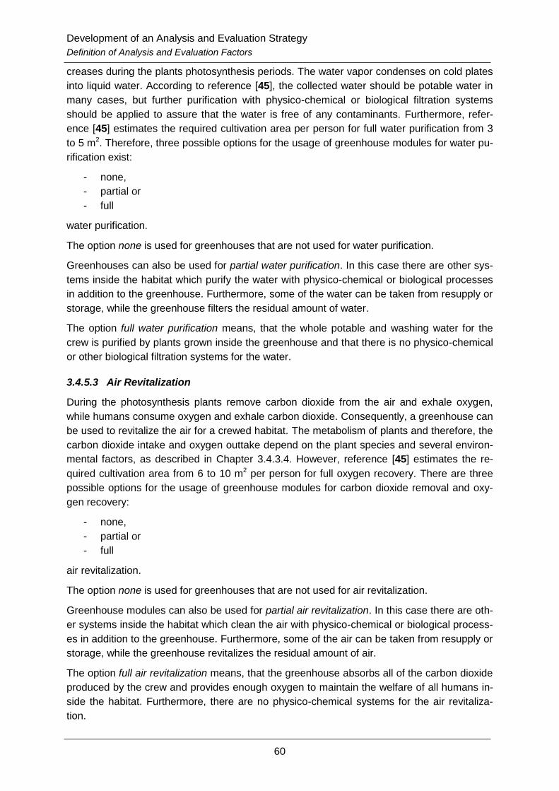
Development of an Analysis and Evaluation Strategy
Definition of Analysis and Evaluation Factors
60
creases during the plants photosynthesis periods. The water vapor condenses on cold plates
into liquid water. According to reference [45], the collected water should be potable water in
many cases, but further purification with physico-chemical or biological filtration systems
should be applied to assure that the water is free of any contaminants. Furthermore, refer-
ence [45] estimates the required cultivation area per person for full water purification from 3
to 5 m2. Therefore, three possible options for the usage of greenhouse modules for water pu-
rification exist:
- none,
- partial or
- full
water purification.
The option none is used for greenhouses that are not used for water purification.
Greenhouses can also be used for partial water purification. In this case there are other sys-
tems inside the habitat which purify the water with physico-chemical or biological processes
in addition to the greenhouse. Furthermore, some of the water can be taken from resupply or
storage, while the greenhouse filters the residual amount of water.
The option full water purification means, that the whole potable and washing water for the
crew is purified by plants grown inside the greenhouse and that there is no physico-chemical
or other biological filtration systems for the water.
3.4.5.3 Air Revitalization
During the photosynthesis plants remove carbon dioxide from the air and exhale oxygen,
while humans consume oxygen and exhale carbon dioxide. Consequently, a greenhouse can
be used to revitalize the air for a crewed habitat. The metabolism of plants and therefore, the
carbon dioxide intake and oxygen outtake depend on the plant species and several environ-
mental factors, as described in Chapter 3.4.3.4. However, reference [45] estimates the re-
quired cultivation area from 6 to 10 m2 per person for full oxygen recovery. There are three
possible options for the usage of greenhouse modules for carbon dioxide removal and oxy-
gen recovery:
- none,
- partial or
- full
air revitalization.
The option none is used for greenhouses that are not used for air revitalization.
Greenhouse modules can also be used for partial air revitalization. In this case there are oth-
er systems inside the habitat which clean the air with physico-chemical or biological process-
es in addition to the greenhouse. Furthermore, some of the air can be taken from resupply or
storage, while the greenhouse revitalizes the residual amount of air.
The option full air revitalization means, that the greenhouse absorbs all of the carbon dioxide
produced by the crew and provides enough oxygen to maintain the welfare of all humans in-
side the habitat. Furthermore, there are no physico-chemical systems for the air revitaliza-
tion.
Development of an Analysis and Evaluation Strategy
Definition of Analysis and Evaluation Factors
61
3.4.5.4 Resupply Dependency
The plant diversity of greenhouse modules describes the type of plants which are cultivated.
The plant types are classified on their ingredients and are similar to the plant categorization
in Chapter 3.4.4.7. Depending on the purpose of the greenhouse module the plant setting
can be composed of plants:
- for fresh food,
- for energy food or
- for a quasi-full nutrition of the crew.
These three categories are the outcome of a trade study made for the Lunar FARM concept
[31], further described in Chapter 4.1.3.
Greenhouse modules with a fresh food plant setup cultivate primarily vegetables with a high
content of water. These vegetables lose quality and palatability after dehydration, stabiliza-
tion and packaging. Consequently, the delivery of them to planetary outposts is not suitable.
In a fresh food scenario crops like wheat or beans are not grown although they are very nu-
trient and efficient. They can easily supplied from Earth, because of their low lose in quality
after dehydration and packaging. However, the high demand of resupply with energy food is
the disadvantage of the fresh food scenario and is therefore, only suitable for short mission
durations or small crews. The cultivation of fresh food is advantageous over nutrition solely
from storage and can be used to cover 26 % of the daily energy intake of the crew. The ben-
efits to the health of the crew are not negligible. Furthermore, the required growth area for
the provision of fresh food is assumed to be 23 m2 per crewmember and the required
crewtime for the work inside the greenhouse module is relatively low compared to the other
two scenarios. Consequently, this scenario should be the least option for a crewed mission to
other planetary bodies [31].
The energy food cultivation scenario can be used for greenhouse modules to produce up to
67 % of the daily energy intake required by the crewmembers. To avoid an imbalance in the
nutrition of the crew the other 33 % of the daily energy intake has to be provided by stored or
supplied food from Earth. In an energy food greenhouse module only plant species with high
energy density and small required growth area are selected for the cultivation. According to
reference [31], eight crops which meet these requirements are beans, carrot, green onion,
pepper, white potato, strawberry, tomato and wheat. The required growth area is estimated
to be around 27 m2 per crewmember. The work load for an energy food greenhouse is higher
than for a fresh food one, but significantly lower than for a quasi-full nutrition scenario. The
energy food option is suitable for medium duration missions [31].
Quasi-full nutrition greenhouses can provide up to 98 % of the daily required energy intake of
the crew. However, some essential vitamins, minerals and proteins have to be provided due
to resupply from Earth. The purpose of this scenario is the achievement of nearly independ-
ency from Earth’s resupply. The pure vegetarian diet and the limitation of some vitamins and
minerals in plants make resupply from Earth indispensable. However, the resupply mass re-
quired is very low compared to the other two scenarios. The required growth area for a qua-
si-full nutrition is assumed to be around 77 m2 per crewmember. Furthermore, the number of
different plant species has to be considered to assure a diversified food composition. Accord-
ing to reference [31], the required crewtime for a quasi-full nutrition greenhouse module is

Development of an Analysis and Evaluation Strategy
Definition of Analysis and Evaluation Factors
62
high and can exceed the available work power of the crew. Therefore, a high level of auto-
mation is necessary for this scenario.
3.4.5.5 Food Provision
The food provision of greenhouse modules is the most important evaluation factors and rep-
resents the amount of edible biomass produced by the plants. The food output is affected by
several environmental and agricultural parameters and additionally depends on the cultivated
plant species. The proposed units for this factor are kilocalories per crewmember per day,
kcal/(CM*d), and gram of dry mass per crewmember per day, g/(CM*d).
3.4.5.6 Power Demand
The intensive lighting required for growing plants causes high power demands for green-
house modules. The required power is primarily dependent on the duration of the lighting pe-
riods and on the chosen lamp types. Usually, the required electrical power is not generated
by the greenhouse modules, but rather generated in special facilities which provide the pow-
er for the whole habitat. Power demands are shown as total power consumption of the mod-
ule in kilowatts, kW, and as power consumption per growth area in kilowatts per square me-
ters, kW/m2. The former value is required for the design of a suitable energy generation facili-
ty, while the latter value is beneficial for the evaluation of different greenhouse module con-
cepts.
3.4.5.7 Cooling Demand
Whether electrical or natural lighting is used as radiation source for plants, the cooling de-
mand is high during the lighting periods. When natural lighting is used, the cooling demand is
affected by the incoming infrared radiation of the sun. In case of electrical lighting, the cool-
ing demand depends on the power demand of the lamps. Nearly all of the electrical energy
required for the lamps is converted to heat. Therefore, it can be assumed, that the cooling
demand is equal to the power demand of the lamps used as radiation source. The proposed
units for the comparison of different greenhouse concepts with respect to the cooling de-
mand are kilowatts, kW, and kilowatts per square meters, kW/m2.
3.4.5.8 Water In-/Output
The water in- and output streams of greenhouses depend on the amount of plants, the plant
species and several environmental conditions. When transpiration water from plants is re-
used as potable or wash water for the crew, or for the watering of the plants, the inwards and
outwards water streams should be nearly equal to each other. The proposed unit for analysis
and evaluation of water in- and output of different greenhouse concepts is kilograms per
square meter per day, kg/(m2*d). The average water streams of greenhouses are estimated
from 5 to 10 kg/(m2*d) in reference [45].
3.4.5.9 Carbon Dioxide Input and Oxygen Output
The carbon dioxide input and the oxygen output of greenhouse modules depend on each
other and on all parameters that influence the photosynthesis of plants. The unit for analyz-
ing and evaluating the streams of CO2 and O2 is kilograms per square meter per day,
kg/(m2*d). The estimated values for the carbon dioxide and oxygen streams are wide spread,
due to the variety of factors that affect the metabolism of plants. However, reference [45]
Development of an Analysis and Evaluation Strategy
Definition of Analysis and Evaluation Factors
63
states the range of carbon dioxide input from 0.04 to 0.30 kg/(m2*d) and the range of oxygen
output from 0.03 to 0.22 kg/(m2*d).
3.4.5.10 Crew Size and Crew Work Load
The factor crew size stands for the amount of humans that one greenhouse module can sup-
port with food, water and air. The supportable crew is directly proportional to the grow area
and efficiency of the greenhouse. The crew size value is required for the normalization of
other parameters and is reported as a number.
The crew work load is the time that the crew needs to fulfill a desired task. Usually, work time
is restricted during space missions. The required time per task is a fix value. Consequently,
the work load can only be lowered by reducing the number of tasks or due to the automation
of processes. Since the number of tasks in greenhouses cannot be lowered without a de-
crease in yield, the work load has to be lowered through automation. Potential options for the
automation of greenhouse modules are discussed in Chapter 3.4.2.7. Table 3-19 shows crew
time values for different greenhouse and domestic activities achieved during the BIOS-3 ex-
periments. Hence, the unit for the time requirement of greenhouse activities is man-hours per
square meter per day, man-hours/(m2*d).
Table 3-19: Crew time requirements for different activities (adapted from BIOS-3) [45]
Activity Time Requirement
Greenhouse Activities [man-hours/(m2*d)]
Planting 0.0199
Harvesting 0.0199
Observation 0.0158
Preventative Maintenance 0.0475
Nutrient Solution Maintenance 0.0300
Wheat Grinding 0.135 man-hours/(d*100 g)
Domestic Activities [man-hours/(CM*d)]
Food Preparation, Eating, Clean-up 1.70
Water Preparation 0.14
Personal Hygiene 0.39
Living Compartment Hygiene 0.27
3.4.5.11 Psychological Health Care
The crew’s psychological health care is an important factor for the success of long-term
space missions and permanent planetary outposts. The permanent isolation from Earth, the
small volume, the potential of system and mission failures, and the risk to die are some of the
broad spectrum of factors that influences the psychological health of the crew. The crew of
spacecraft are tested and trained for the stresses of space missions, but nevertheless they
are not immune to psychological sicknesses. Studies with small greenhouses onboard the
MIR station and the ISS indicate that the crew’s sentiment benefits from handling, growing
and taking care of plants [12]. Besides the crew, plants are the only living creatures onboard

Development of an Analysis and Evaluation Strategy
Summary
64
a spacecraft. According to reference [51], Space Shuttle astronaut Mike Foale loved the ex-
periments with greenhouses, because they reduced his irritability. Furthermore, reference
[12] cites Salyut cosmonaut Valentin Lebedev, that plants were like pets for him during his
missions.
Consequently, a greenhouse has to be designed to offer benefits for the psyche of the crew
in addition to the provision of food, water and air. The interaction with the plants in a techni-
cally dominated environment passively offers benefits to the psyche of the crew [43]. Fur-
thermore, special plants can be grown. Spices have a strong effect on the well-being of the
crew, because they can make the commonly monotone food tastier. In addition, the provision
of incentive food that is not required for the nutrition of the crew can improve the psyche of
the crew [51]. When investigated greenhouse module concepts consider the psyche of the
crew. The implemented options have to be investigated.
3.5 Summary
Chapter 3 starts with the description of the analysis and evaluation strategy proposed in this
thesis in the first subchapter. For the developed methodology an analysis and one or more
evaluation methods are required.
The second subchapter describes the selected analysis method, the Morphological Analysis
(MA). The MA is suitable for the analysis of greenhouse modules, because it allows a sys-
tematic analysis of current and future options for the defined subsystems. Furthermore, the
MA provides a multitude of combinations and permutations for the analysis goal and there-
fore, a framework for the following evaluation. The result of a MA is a Morphological Box
which is hierarchically structured and provides an overview over all measurable factors relat-
ed to the goal of the analysis.
The third subchapter introduces two suitable evaluation methods for greenhouse modules.
The first one, the Equivalent System Mass (ESM), is developed for the evaluation of ECLSS
and is advantageous for evaluation with respect to transportation costs. However, the ESM
method cannot be used for the evaluation of qualitative and performance criteria. The second
evaluation method, the Analytical Hierarchy Process (AHP), is a more general evaluation
method. The AHP requires defined evaluation criteria, whereby qualitative and quantitative
criteria can be established. The criteria are arranged in a hierarchy. For the reduction of bias,
the weighting of the criteria can be executed with a group of experts. Consequently, the AHP
is selected for the evaluation of greenhouse module concepts conducted in Chapter 4.
The fourth subchapter establishes analysis and evaluation factors for greenhouse modules
and a detailed description for each factor is given. The factors are grouped to four major cat-
egories: fundamental factors, environmental factors, agricultural factors and interface factors.
The factors can be divided in qualitative and quantitative factors. In total 46 measurable fac-
tors are identified during this thesis, 13 fundamental, 11 environmental, 10 agricultural and
12 interface factors. Table 3-20 shows a complete summary of all established factors and
their possible options, respectively units. Thereby, the factors are arranged in a Morphologi-
cal Box.
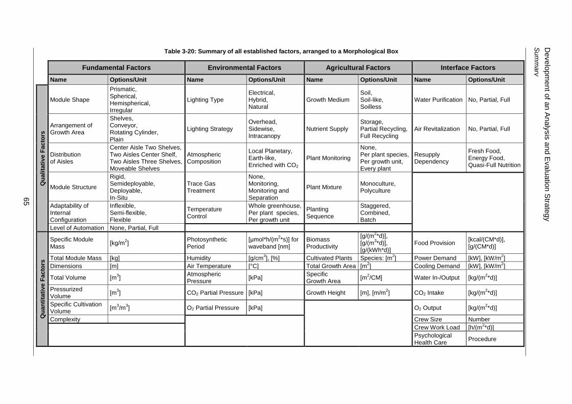
Table 3-20: Summary of all established factors, arranged to a Morphological Box
Fundamental Factors Environmental Factors Agricultural Factors Interface Factors
Name Options/Unit Name Options/Unit Name Options/Unit Name Options/Unit
Qu
ali
tati
ve
Fa
cto
rs
Module Shape
Prismatic, Spherical, Hemispherical, Irregular
Lighting Type Electrical, Hybrid, Natural
Growth Medium Soil, Soil-like, Soilless
Water Purification No, Partial, Full
Arrangement of Growth Area
Shelves, Conveyor, Rotating Cylinder, Plain
Lighting Strategy Overhead, Sidewise, Intracanopy
Nutrient Supply Storage, Partial Recycling, Full Recycling
Air Revitalization No, Partial, Full
Distribution of Aisles
Center Aisle Two Shelves, Two Aisles Center Shelf, Two Aisles Three Shelves, Moveable Shelves
Atmospheric Composition
Local Planetary, Earth-like, Enriched with CO2
Plant Monitoring
None, Per plant species, Per growth unit, Every plant
Resupply Dependency
Fresh Food, Energy Food, Quasi-Full Nutrition
Module Structure
Rigid, Semideployable, Deployable, In-Situ
Trace Gas Treatment
None, Monitoring, Monitoring and Separation
Plant Mixture Monoculture, Polyculture
Adaptability of Internal Configuration
Inflexible, Semi-flexible, Flexible
Temperature Control
Whole greenhouse, Per plant species, Per growth unit
Planting Sequence
Staggered, Combined, Batch
Level of Automation None, Partial, Full
Qu
an
tita
tive
Fa
cto
rs
Specific Module Mass
[kg/m2]
Photosynthetic Period
[μmol*h/(m2*s)] for
waveband [nm] Biomass Productivity
[g/(m2*d)],
[g/(m3*d)],
[g/(kWh*d)] Food Provision
[kcal/(CM*d)], [g/(CM*d)]
Total Module Mass [kg] Humidity [g/cm3], [%] Cultivated Plants Species: [m
2] Power Demand [kW], [kW/m
2]
Dimensions [m] Air Temperature [°C] Total Growth Area [m2] Cooling Demand [kW], [kW/m
2]
Total Volume [m3]
Atmospheric Pressure
[kPa] Specific Growth Area
[m2/CM] Water In-/Output [kg/(m
2*d)]
Pressurized Volume
[m3] CO2 Partial Pressure [kPa] Growth Height [m], [m/m
2] CO2 Intake [kg/(m
2*d)]
Specific Cultivation Volume
[m3/m
3] O2 Partial Pressure [kPa] O2 Output [kg/(m
2*d)]
Complexity Crew Size Number
Crew Work Load [h/(m2*d)]
Psychological Health Care
Procedure
65
De
velo
pm
en
t of a
n A
naly
sis
and
Eva
luatio
n S
trate
gy
Sum
mary

Demonstration of the Developed Evaluation Strategy
Description and Analysis of Selected Concepts and Testbeds
66
4 Demonstration of the Developed Evaluation Strategy
In this chapter a survey of existing greenhouse concepts is accomplished in the first sub-
chapter. Three of these concepts are selected for further investigation. The second subchap-
ter describes the goal of the demonstrated evaluation. The third subchapter establishes the
evaluation criteria and the local and global weighting values for each criterion. In the fourth
subchapter the weighted evaluation criteria are used in an AHP to evaluate the selected con-
cepts.
4.1 Description and Analysis of Selected Concepts and Testbeds
4.1.1 Survey on Existing Greenhouse Concepts
One of the common definitions of a greenhouse can be found in reference [52]: “A green-
house has one purpose: to provide and maintain the environment that will result in optimum
crop production or maximum profit. This includes an environment for work efficiency as well
as for crop growth.” This statement defines the purpose of terrestrial and space greenhouses
correctly. However, plant cultivation systems for space applications can differ from the above
mentioned definition. Systems for plant cultivation in space are broadly divided into plant
growth chambers (PGC) and greenhouse modules (GHM).
Plant Growth Chambers are usually systems with a small cultivation area of less than one
square meter. The main purpose of today’s PGCs is the research of plant development and
growing in a controlled environment under micro gravity. Other purposes of these chambers
is the testing and verification of subsystems in space, the interaction between crew members
and plants, and the psychological effect of plants in a sterile, highly technical environment.
The plants cultivated in PGCs can be edible and inedible, depending on the purpose. How-
ever, the amount of produced edible biomass is generally low and can only be used as an
addition to the normal food. Table 4-1 shows a list of some plant growth chambers and their
key parameters.
Greenhouses are large systems or even independent modules of space stations or planetary
habitats. The purpose of a GHM is the provision of edible biomass to the crew to reduce the
required resupply mass of food. Depending on the mission requirements and the system de-
sign, GHMs can produce different sets of crops ranging from fresh vegetables for short dura-
tion missions over energy food for medium duration missions up to quasi-full nutrition for long
duration missions or permanent planetary habitats. Furthermore, GHMs can be used as part
of the ECLSS. The plants of a GHM can purify water, revitalize air and recycle some of the
bio waste of the crew. As shown in Chapter 2.3 BLSS and therefore, GHMs are required for
long duration and permanent extraterrestrial human settlements.
The variety of GHM concepts and test facilities is high. They can to be divided depending on
their purpose and location into the four groups:
- Terrestrial plant cultivation test facilities,
- Terrestrial human isolation test facilities,
- Arctic and Antarctic plant cultivation test facilities,
- Greenhouse module concepts for space application.
Terrestrial plant cultivation test facilities are designed to research plant cultivation in a con-
trolled environment on Earth. Research in plant growing and subsystem development are the
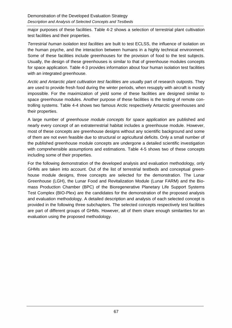
Demonstration of the Developed Evaluation Strategy
Description and Analysis of Selected Concepts and Testbeds
67
major purposes of these facilities. Table 4-2 shows a selection of terrestrial plant cultivation
test facilities and their properties.
Terrestrial human isolation test facilities are built to test ECLSS, the influence of isolation on
the human psyche, and the interaction between humans in a highly technical environment.
Some of these facilities include greenhouses for the provision of food to the test subjects.
Usually, the design of these greenhouses is similar to that of greenhouse modules concepts
for space application. Table 4-3 provides information about four human isolation test facilities
with an integrated greenhouse.
Arctic and Antarctic plant cultivation test facilities are usually part of research outposts. They
are used to provide fresh food during the winter periods, when resupply with aircraft is mostly
impossible. For the maximization of yield some of these facilities are designed similar to
space greenhouse modules. Another purpose of these facilities is the testing of remote con-
trolling systems. Table 4-4 shows two famous Arctic respectively Antarctic greenhouses and
their properties.
A large number of greenhouse module concepts for space application are published and
nearly every concept of an extraterrestrial habitat includes a greenhouse module. However,
most of these concepts are greenhouse designs without any scientific background and some
of them are not even feasible due to structural or agricultural deficits. Only a small number of
the published greenhouse module concepts are undergone a detailed scientific investigation
with comprehensible assumptions and estimations. Table 4-5 shows two of these concepts
including some of their properties.
For the following demonstration of the developed analysis and evaluation methodology, only
GHMs are taken into account. Out of the list of terrestrial testbeds and conceptual green-
house module designs, three concepts are selected for the demonstration. The Lunar
Greenhouse (LGH), the Lunar Food and Revitalization Module (Lunar FARM) and the Bio-
mass Production Chamber (BPC) of the Bioregenerative Planetary Life Support Systems
Test Complex (BIO-Plex) are the candidates for the demonstration of the proposed analysis
and evaluation methodology. A detailed description and analysis of each selected concept is
provided in the following three subchapters. The selected concepts respectively test facilities
are part of different groups of GHMs. However, all of them share enough similarities for an
evaluation using the proposed methodology.
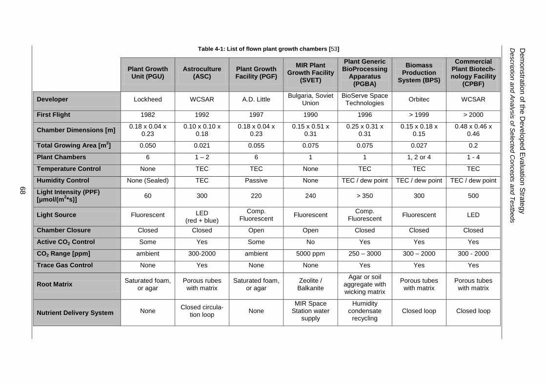
Table 4-1: List of flown plant growth chambers [53]
Plant Growth
Unit (PGU) Astroculture
(ASC) Plant Growth Facility (PGF)
MIR Plant Growth Facility
(SVET)
Plant Generic BioProcessing
Apparatus (PGBA)
Biomass Production
System (BPS)
Commercial Plant Biotech-nology Facility
(CPBF)
Developer Lockheed WCSAR A.D. Little Bulgaria, Soviet
Union BioServe Space
Technologies Orbitec WCSAR
First Flight 1982 1992 1997 1990 1996 > 1999 > 2000
Chamber Dimensions [m] 0.18 x 0.04 x
0.23 0.10 x 0.10 x
0.18 0.18 x 0.04 x
0.23 0.15 x 0.51 x
0.31 0.25 x 0.31 x
0.31 0.15 x 0.18 x
0.15 0.48 x 0.46 x
0.46
Total Growing Area [m2] 0.050 0.021 0.055 0.075 0.075 0.027 0.2
Plant Chambers 6 1 – 2 6 1 1 1, 2 or 4 1 - 4
Temperature Control None TEC TEC None TEC TEC TEC
Humidity Control None (Sealed) TEC Passive None TEC / dew point TEC / dew point TEC / dew point
Light Intensity (PPF) [μmol/(m
2*s)]
60 300 220 240 > 350 300 500
Light Source Fluorescent LED (red + blue)
Comp. Fluorescent
Fluorescent Comp.
Fluorescent Fluorescent LED
Chamber Closure Closed Closed Open Open Closed Closed Closed
Active CO2 Control Some Yes Some No Yes Yes Yes
CO2 Range [ppm] ambient 300-2000 ambient 5000 ppm 250 – 3000 300 – 2000 300 - 2000
Trace Gas Control None Yes None None Yes Yes Yes
Root Matrix Saturated foam,
or agar Porous rubes
with matrix Saturated foam,
or agar Zeolite / Balkanite
Agar or soil aggregate with wicking matrix
Porous tubes with matrix
Porous tubes with matrix
Nutrient Delivery System None Closed circula-
tion loop None
MIR Space Station water
supply
Humidity condensate
recycling Closed loop Closed loop
68
De
mo
nstra
tion
of th
e D
evelo
pe
d E
va
luatio
n S
trate
gy
Descrip
tion a
nd A
naly
sis
of S
ele
cte
d C
oncepts
and T
estb
eds

Table 4-2: List of terrestrial plant cultivation test facilities
Terrestrial Test Facility Organization Research Focus Greenhouse Parameter References
CLESS Experimental Facility (Since 2004)
Department of ECLSS, China Astronaut Research & Training Center (Beijing, China)
Plant cultivation in closed loop & plant-human integrat-ed experiments.
Total Cultivation Area 8.4 m²
[54]
Temperature 15 – 40 °C
Relative Humidity 65 – 85 %
CO2 Concentration 350 – 10000 ppm
Total Pressure Earth-Like
Lighting LED (95 % red, 5 % blue)
PPF 0 – 500 µmol/(m2*s)
Growth Medium Hydroponic
Biomass Production Chamber (1988 – 1996)
NASA Kennedy Space Center (Florida, USA)
Provides an unique oppor-tunity to learn about the mass and energy flow though the CELSS along with the environmental needs for plant growth in a con-cealed environment.
Total Cultivation Area 20 m²
[55], [56], [57]
Temperature 23 °C
Relative Humidity 70 – 80 %
CO2 Concentration 1000 – 1200 ppm
Total Pressure Earth-Like
Lighting 96x 400 W HID Lamps
PPF 200 – 700 µmol/(m2*s)
Growth Medium Hydroponic
Lunar Greenhouse (Since 2005)
Controlled Environment Agriculture Center, University of Arizona & Sadler Machine Company (Tucson, Arizona, USA)
Demonstration of maximum biomass generation and food production within a poly-culture deployable cropping system. Furthermore, com-plete water recycling and revitalization of interior at-mosphere.
Total Cultivation Area 8.8 m²
[58], [59]
Temperature 21.1 °C
Relative Humidity 53.5 %
CO2 Concentration 1000 ppm
Total Pressure Earth-Like
Lighting 6x 1000 W HPS
PPF 300 – 400 µmol/(m2*s)
Growth Medium Hydroponic
69
De
mo
nstra
tion o
f the D
evelo
pe
d E
va
luatio
n S
trate
gy
De
scrip
tion a
nd A
naly
sis
of S
ele
cte
d C
once
pts
an
d T
estb
ed
s
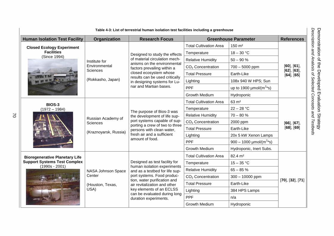
Table 4-3: List of terrestrial human isolation test facilities including a greenhouse
Human Isolation Test Facility Organization Research Focus Greenhouse Parameter References
Closed Ecology Experiment Facilities
(Since 1994)
Institute for Environmental Sciences (Rokkasho, Japan)
Designed to study the effects of material circulation mech-anisms on the environmental factors prevailing within a closed ecosystem whose results can be used critically in designing systems for Lu-nar and Martian bases.
Total Cultivation Area 150 m²
[60], [61], [62], [63], [64], [65]
Temperature 18 – 30 °C
Relative Humidity 50 – 90 %
CO2 Concentration 700 – 5000 ppm
Total Pressure Earth-Like
Lighting 108x 940 W HPS; Sun
PPF up to 1900 µmol/(m2*s)
Growth Medium Hydroponic
BIOS-3 (1972 – 1984)
Russian Academy of Sciences (Kraznoyarsk, Russia)
The purpose of Bios-3 was the development of life sup-port systems capable of sup-porting a crew of two to three persons with clean water, fresh air and a sufficient amount of food.
Total Cultivation Area 63 m²
[66], [67], [68], [69]
Temperature 22 – 28 °C
Relative Humidity 70 – 80 %
CO2 Concentration 2000 ppm
Total Pressure Earth-Like
Lighting 20x 5 kW Xenon Lamps
PPF 900 – 1000 µmol/(m2*s)
Growth Medium Hydroponic, Inert Subs.
Bioregenerative Planetary Life Support Systems Test Complex
(1990s - 2001)
NASA Johnson Space Center (Houston, Texas, USA)
Designed as test facility for human isolation experiments and as a testbed for life sup-port systems. Food produc-tion, water purification and air revitalization and other key elements of an ECLSS can be evaluated during long duration experiments.
Total Cultivation Area 82.4 m²
[70], [32], [71]
Temperature 15 – 35 °C
Relative Humidity 65 – 85 %
CO2 Concentration 300 – 10000 ppm
Total Pressure Earth-Like
Lighting 384 HPS Lamps
PPF n/a
Growth Medium Hydroponic
70
De
mo
nstra
tion
of th
e D
evelo
pe
d E
va
luatio
n S
trate
gy
Descrip
tion a
nd A
naly
sis
of S
ele
cte
d C
oncepts
and T
estb
eds
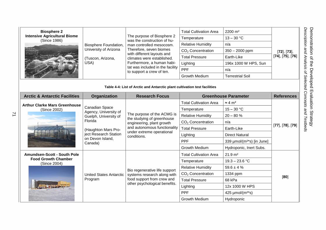
Biosphere 2 Intensive Agricultural Biome
(Since 1986)
Biosphere Foundation, University of Arizona (Tuscon, Arizona, USA)
The purpose of Biosphere 2 was the construction of hu-man controlled mesocosm. Therefore, seven biomes with different layouts and climates were established. Furthermore, a human habi-tat was included in the facility to support a crew of ten.
Total Cultivation Area 2200 m²
[72], [73], [74], [75], [76]
Temperature 13 – 30 °C
Relative Humidity n/a
CO2 Concentration 350 – 2000 ppm
Total Pressure Earth-Like
Lighting 196x 1000 W HPS, Sun
PPF n/a
Growth Medium Terrestrial Soil
Table 4-4: List of Arctic and Antarctic plant cultivation test facilities
Arctic & Antarctic Facilities Organization Research Focus Greenhouse Parameter References
Arthur Clarke Mars Greenhouse (Since 2002)
Canadian Space Agency, University of Guelph, University of Florida (Haughton Mars Pro-ject Research Station on Devon Island, Canada)
The purpose of the ACMG is the studying of greenhouse engineering, plant growth and autonomous functionality under extreme operational conditions.
Total Cultivation Area ≈ 4 m²
[77], [78], [79]
Temperature 15 – 30 °C
Relative Humidity 20 – 80 %
CO2 Concentration n/a
Total Pressure Earth-Like
Lighting Direct Natural
PPF 339 µmol/(m²*s) [in June]
Growth Medium Hydroponic, Inert Subs.
Amundsen-Scott - South Pole Food Growth Chamber
(Since 2004)
United States Antarctic Program
Bio regenerative life support systems research along with food support from crew and other psychological benefits.
Total Cultivation Area 21.9 m²
[80]
Temperature 19.3 – 23.6 °C
Relative Humidity 59.6 ± 4 %
CO2 Concentration 1334 ppm
Total Pressure 68 kPa
Lighting 12x 1000 W HPS
PPF 425 µmol/(m²*s)
Growth Medium Hydroponic
71
De
mo
nstra
tion
of th
e D
evelo
pe
d E
va
luatio
n S
trate
gy
Descrip
tion a
nd A
naly
sis
of S
ele
cte
d C
oncepts
and T
estb
eds

Table 4-5: List of greenhouse module concepts for space applications
GHM for Space Application Organization Research Focus Greenhouse Parameter References
Lunar Food and Air Revitalization Module
(2008)
2nd International Master Course in Space Exploration and Development Systems (SEEDS) (Mt. Malapert, Lunar South Pole)
Designed as a plant growth chamber module to be inte-grated into the Bio regenera-tive life support systems for a Lunar Mission.
Total Cultivation Area 144 m²
[31], [81], [82]
Temperature 17 – 28 °C
Relative Humidity 25 – 75 %
CO2 Concentration 265 ppm
Total Pressure 75.5 kPa
Lighting Indirect Natural, HPS
PPF n/a
Growth Medium Hydroponic
Autonomous Garden Pod (2002)
NASA Mars Port Competition, University of Colorado (Colorado, USA)
Designed as inflatable plant growth chamber module to be integrated into the Bio regenerative life support sys-tems for a Martian Mission.
Total Cultivation Area 9.9 m²
[83]
Temperature n/a
Relative Humidity n/a
CO2 Concentration CO2 rich atmosphere
Total Pressure n/a
Lighting Direct, Indirect Natural
PPF n/a
Growth Medium n/a
72
De
mo
nstra
tion
of th
e D
evelo
pe
d E
va
luatio
n S
trate
gy
Descrip
tion a
nd A
naly
sis
of S
ele
cte
d C
oncepts
and T
estb
eds

Demonstration of the Developed Evaluation Strategy
Description and Analysis of Selected Concepts and Testbeds
73
4.1.2 Lunar Greenhouse
The Lunar Greenhouse (LGH) is a BLSS concept developed by an U.S.-Italian corporation
under the leadership of the University of Arizona’s Controlled Environment Agriculture Center
(UA-CEAC). Other partners are Sadler Machine Company, Thales Alenia Space-Italia, Aero-
Sekur, and the University of Naples Federico II. The project started in 2005 with a feasibility
study and is still running. According to reference [58], the purpose of the Lunar Greenhouse
project is the demonstration of biomass and food production, air and water revitalization, and
waste recycling within a poly-culture deployable cropping system.
The module is designed to meet the requirements for a lunar science outpost established by
NASA’s Global Exploration Strategy. This scenario proposes a lunar outpost with four LGH
modules at the Aitken Basin near the Lunar South Pole for a 4-person crew and mission du-
ration of 180 days. The aim of the greenhouse for this scenario is full water purification and
air revitalization, and the provision of up to 50 % of the required daily energy intake of the
crew. The greenhouse module concept discussed in this chapter is able to fulfill these re-
quirements for one human. Consequently, four modules are required to meet the require-
ments for the lunar outpost scenario [58].
The module consists of a deployable aluminum structure and has a cylindrical shape. Figure
4-1 shows a prototype of the LGH in folded configuration, while Figure 4-2 illustrates the
module fully deployed and operational during a test phase. For outer shell of the module a
fluorocarbon based polymer membrane is used. Due to the absence of a rigid outer shell, the
module has to be covered with one meter of lunar soil to prevent the plants against the cos-
mic radiation. While deployed, the LGH has a length of 5.5 meters and a diameter of 2.06
meters. Consequently, the pressurized volume is around 21 cubic meters [58].
Figure 4-1: Folded Configuration of
the LGH [59]
Figure 4-2: Deployed Configuration of the LGH during a test
period [59]
The growth area is accommodated in two one-level shelves, one at each side of the centered
aisle. The overall cultivation area of one module is around 8.8 square meters. When the aisle
is also be used as growth area, 11.1 square meters growth area are available. The available
growth height depends, due to the cylindrical shape, on the distance to the outer shell. The
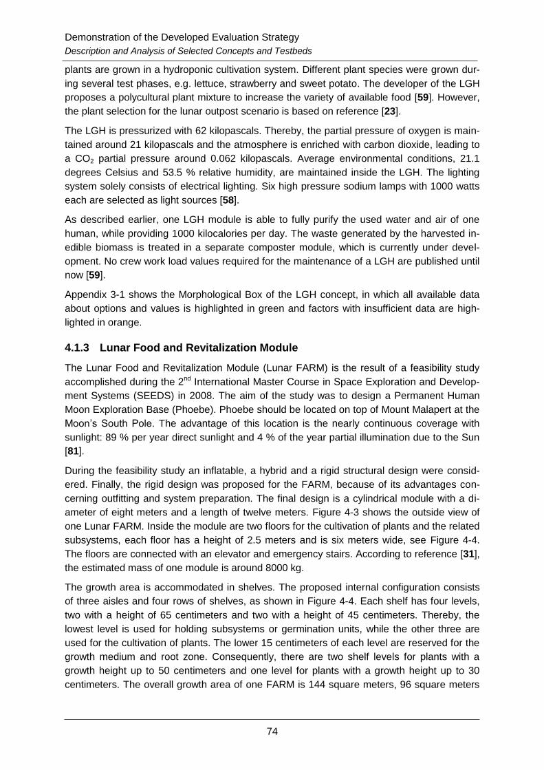
Demonstration of the Developed Evaluation Strategy
Description and Analysis of Selected Concepts and Testbeds
74
plants are grown in a hydroponic cultivation system. Different plant species were grown dur-
ing several test phases, e.g. lettuce, strawberry and sweet potato. The developer of the LGH
proposes a polycultural plant mixture to increase the variety of available food [59]. However,
the plant selection for the lunar outpost scenario is based on reference [23].
The LGH is pressurized with 62 kilopascals. Thereby, the partial pressure of oxygen is main-
tained around 21 kilopascals and the atmosphere is enriched with carbon dioxide, leading to
a CO2 partial pressure around 0.062 kilopascals. Average environmental conditions, 21.1
degrees Celsius and 53.5 % relative humidity, are maintained inside the LGH. The lighting
system solely consists of electrical lighting. Six high pressure sodium lamps with 1000 watts
each are selected as light sources [58].
As described earlier, one LGH module is able to fully purify the used water and air of one
human, while providing 1000 kilocalories per day. The waste generated by the harvested in-
edible biomass is treated in a separate composter module, which is currently under devel-
opment. No crew work load values required for the maintenance of a LGH are published until
now [59].
Appendix 3-1 shows the Morphological Box of the LGH concept, in which all available data
about options and values is highlighted in green and factors with insufficient data are high-
lighted in orange.
4.1.3 Lunar Food and Revitalization Module
The Lunar Food and Revitalization Module (Lunar FARM) is the result of a feasibility study
accomplished during the 2nd International Master Course in Space Exploration and Develop-
ment Systems (SEEDS) in 2008. The aim of the study was to design a Permanent Human
Moon Exploration Base (Phoebe). Phoebe should be located on top of Mount Malapert at the
Moon’s South Pole. The advantage of this location is the nearly continuous coverage with
sunlight: 89 % per year direct sunlight and 4 % of the year partial illumination due to the Sun
[81].
During the feasibility study an inflatable, a hybrid and a rigid structural design were consid-
ered. Finally, the rigid design was proposed for the FARM, because of its advantages con-
cerning outfitting and system preparation. The final design is a cylindrical module with a di-
ameter of eight meters and a length of twelve meters. Figure 4-3 shows the outside view of
one Lunar FARM. Inside the module are two floors for the cultivation of plants and the related
subsystems, each floor has a height of 2.5 meters and is six meters wide, see Figure 4-4.
The floors are connected with an elevator and emergency stairs. According to reference [31],
the estimated mass of one module is around 8000 kg.
The growth area is accommodated in shelves. The proposed internal configuration consists
of three aisles and four rows of shelves, as shown in Figure 4-4. Each shelf has four levels,
two with a height of 65 centimeters and two with a height of 45 centimeters. Thereby, the
lowest level is used for holding subsystems or germination units, while the other three are
used for the cultivation of plants. The lower 15 centimeters of each level are reserved for the
growth medium and root zone. Consequently, there are two shelf levels for plants with a
growth height up to 50 centimeters and one level for plants with a growth height up to 30
centimeters. The overall growth area of one FARM is 144 square meters, 96 square meters
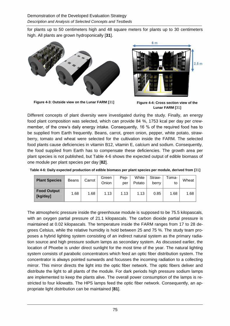
Demonstration of the Developed Evaluation Strategy
Description and Analysis of Selected Concepts and Testbeds
75
for plants up to 50 centimeters high and 48 square meters for plants up to 30 centimeters
high. All plants are grown hydroponically [31].
Figure 4-3: Outside view on the Lunar FARM [31]
Figure 4-4: Cross section view of the
Lunar FARM [31]
Different concepts of plant diversity were investigated during the study. Finally, an energy
food plant composition was selected, which can provide 84 %, 1753 kcal per day per crew-
member, of the crew’s daily energy intake. Consequently, 16 % of the required food has to
be supplied from Earth frequently. Beans, carrot, green onion, pepper, white potato, straw-
berry, tomato and wheat were selected for the cultivation inside the FARM. The selected
food plants cause deficiencies in vitamin B12, vitamin E, calcium and sodium. Consequently,
the food supplied from Earth has to compensate these deficiencies. The growth area per
plant species is not published, but Table 4-6 shows the expected output of edible biomass of
one module per plant species per day [82].
Table 4-6: Daily expected production of edible biomass per plant species per module, derived from [31]
Plant Species Beans Carrot Green
Onion
Pep-
per
White
Potato
Straw-
berry
Toma-
to Wheat
Food Output
[kg/day] 1.68 1.68 1.13 1.13 1.13 0.85 1.68 1.68
The atmospheric pressure inside the greenhouse module is supposed to be 75.5 kilopascals,
with an oxygen partial pressure of 21.1 kilopascals. The carbon dioxide partial pressure is
maintained at 0.02 kilopascals. The temperature inside the FARM ranges from 17 to 28 de-
grees Celsius, while the relative humidity is hold between 25 and 75 %. The study team pro-
poses a hybrid lighting system consisting of an indirect natural system as the primary radia-
tion source and high pressure sodium lamps as secondary system. As discussed earlier, the
location of Phoebe is under direct sunlight for the most time of the year. The natural lighting
system consists of parabolic concentrators which feed an optic fiber distribution system. The
concentrator is always pointed sunwards and focusses the incoming radiation to a collecting
mirror. This mirror directs the light into the optic fiber network. The optic fibers deliver and
distribute the light to all plants of the module. For dark periods high pressure sodium lamps
are implemented to keep the plants alive. The overall power consumption of the lamps is re-
stricted to four kilowatts. The HPS lamps feed the optic fiber network. Consequently, an ap-
propriate light distribution can be maintained [81].

Demonstration of the Developed Evaluation Strategy
Description and Analysis of Selected Concepts and Testbeds
76
The FARM was designed to grow food plants for the nourishment of Phoebe’s crew. The
proposed crew composition is 50 % men and 50 % women and a permanent crew size of 18
people. Furthermore, during crew exchange six additional humans will live in Phoebe for 14
days. The crew exchange was supposed to be every eight weeks. In addition to the crew ex-
change, six visitors will stay at the base for seven days every eight weeks. However, crew
exchange and visiting should never overlap, which leads to a maximum crew size of 24. For
the provision of food to the desired crew size four FARMs are required. Besides the plant cul-
tivation the FARM is used to purify the water and revitalize the air of the whole habitat. The
water output is estimated to be around 36 kilograms per day and the amount of generated
oxygen is calculated to 1.0 kg per crewmember per day. To maintain all functions of one
module and to grow and harvest the desired amount of food, reference [31] assumes a work-
load of ten man-hours per day for the whole module. Consequently, the crew work load is
around 0.07 man hours per square meter per day.
Appendix 3-2 shows the Morphological Box of the Lunar FARM concept, in which all availa-
ble data about options and values is highlighted in green and factors with insufficient data are
highlighted in orange.
4.1.4 Biomass Production Chamber of BIO-Plex
The Bioregenerative Planetary Life Support Systems Test Complex (BIO-Plex) is one of
NASA’s projects of the Advanced Life Support (ALS) program and is located at the Johnson
Space Center (JSC) in Houston. BIO-Plex is designed as test facility for human isolation ex-
periments and as a testbed for life support systems. Systems regarding the food production,
water purification and air revitalization and other key elements of an ECLSS can be integrat-
ed and evaluated during long duration experiments. The purpose of BIO-Plex is the provision
of a closed environment including a small crew for the testing of current and future regenera-
ble systems technologies. The design of the facility began in the early 1990s, but the project
was directed to suspend ongoing activities in 2001 due to the declining NASA budget. Since
2001 the built parts of the facility are placed in a “stand-by” mode. [70].
BIO-Plex consists of six cylindrical chambers and an airlock connected to an interconnecting
tunnel. Figure 4-5 shows an outside view on BIO-Plex during the integration. The transparent
airlock is attached on the right side, while two modules on the left side are still missing. Each
of the six chambers has a different purpose. The habitation chamber accommodates the
crew quarters. The life support chamber contains all systems required to maintain the de-
sired environmental conditions, while the utilities distribution module serves as storage room
for tools. A laboratory chamber is proposed for a later development stage of the complex.
Furthermore, BIO-Plex has two Biomass Production Chambers (BPC). Hence, the BPC de-
sign is described in detail in the following [32].
The BPC has a rigid cylindrical structure as every chamber of BIO-Plex, is 11.3 meters long
and has a diameter of 4.6 meters. Consequently, the BPC has a pressurized volume of 187.8
cubic meters. Most of the crop processing systems are located inside the interconnecting
tunnel. Consequently, a wider door, 168 centimeters, compared to the other chambers is in-
stalled between the BPC and the interconnecting tunnel, which facilitates an easier handling
of seedlings, plants and harvested crops [32].
The growth area is accommodated in shelves. Therefore, four shelf designs were considered
during the design process. Finally, a two aisles three shelves configuration was selected as
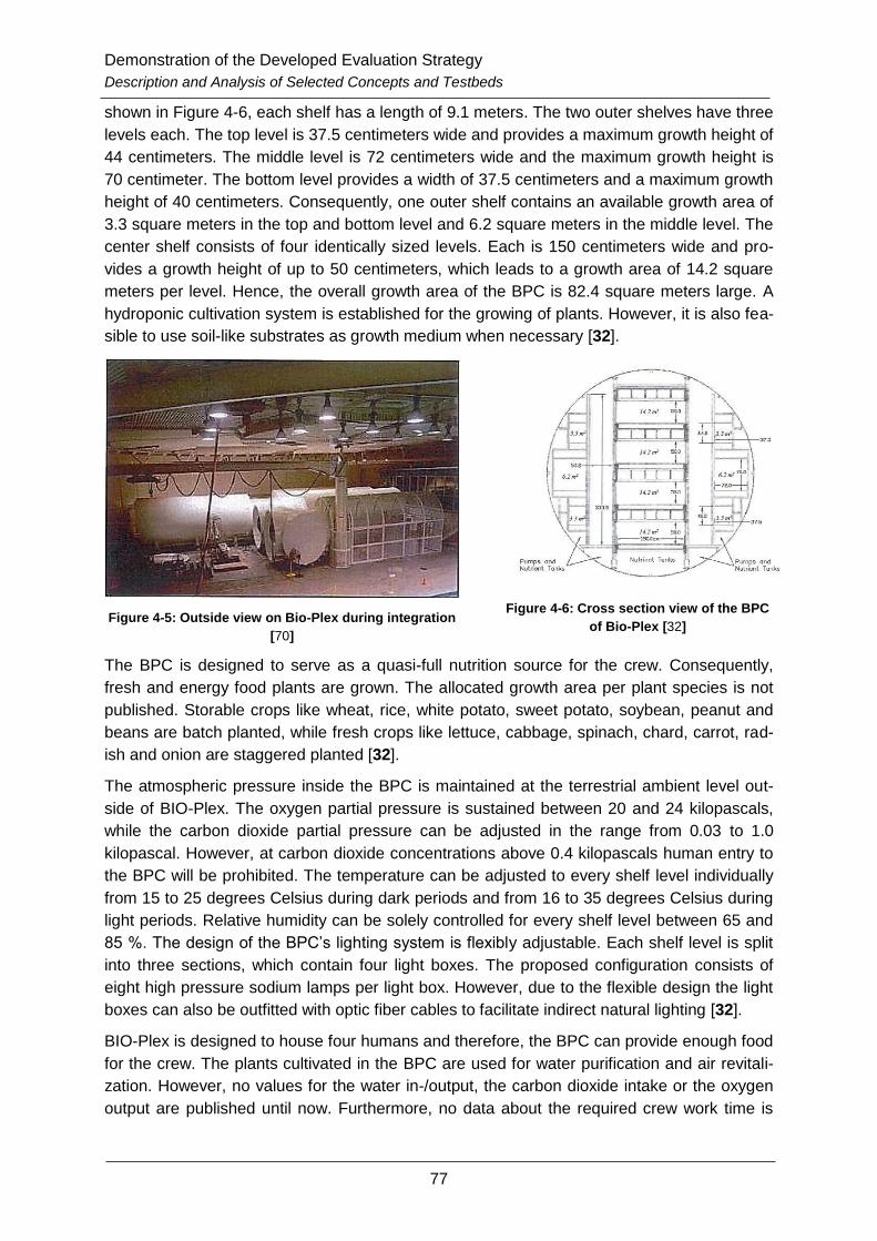
Demonstration of the Developed Evaluation Strategy
Description and Analysis of Selected Concepts and Testbeds
77
shown in Figure 4-6, each shelf has a length of 9.1 meters. The two outer shelves have three
levels each. The top level is 37.5 centimeters wide and provides a maximum growth height of
44 centimeters. The middle level is 72 centimeters wide and the maximum growth height is
70 centimeter. The bottom level provides a width of 37.5 centimeters and a maximum growth
height of 40 centimeters. Consequently, one outer shelf contains an available growth area of
3.3 square meters in the top and bottom level and 6.2 square meters in the middle level. The
center shelf consists of four identically sized levels. Each is 150 centimeters wide and pro-
vides a growth height of up to 50 centimeters, which leads to a growth area of 14.2 square
meters per level. Hence, the overall growth area of the BPC is 82.4 square meters large. A
hydroponic cultivation system is established for the growing of plants. However, it is also fea-
sible to use soil-like substrates as growth medium when necessary [32].
Figure 4-5: Outside view on Bio-Plex during integration
[70]
Figure 4-6: Cross section view of the BPC
of Bio-Plex [32]
The BPC is designed to serve as a quasi-full nutrition source for the crew. Consequently,
fresh and energy food plants are grown. The allocated growth area per plant species is not
published. Storable crops like wheat, rice, white potato, sweet potato, soybean, peanut and
beans are batch planted, while fresh crops like lettuce, cabbage, spinach, chard, carrot, rad-
ish and onion are staggered planted [32].
The atmospheric pressure inside the BPC is maintained at the terrestrial ambient level out-
side of BIO-Plex. The oxygen partial pressure is sustained between 20 and 24 kilopascals,
while the carbon dioxide partial pressure can be adjusted in the range from 0.03 to 1.0
kilopascal. However, at carbon dioxide concentrations above 0.4 kilopascals human entry to
the BPC will be prohibited. The temperature can be adjusted to every shelf level individually
from 15 to 25 degrees Celsius during dark periods and from 16 to 35 degrees Celsius during
light periods. Relative humidity can be solely controlled for every shelf level between 65 and
85 %. The design of the BPC’s lighting system is flexibly adjustable. Each shelf level is split
into three sections, which contain four light boxes. The proposed configuration consists of
eight high pressure sodium lamps per light box. However, due to the flexible design the light
boxes can also be outfitted with optic fiber cables to facilitate indirect natural lighting [32].
BIO-Plex is designed to house four humans and therefore, the BPC can provide enough food
for the crew. The plants cultivated in the BPC are used for water purification and air revitali-
zation. However, no values for the water in-/output, the carbon dioxide intake or the oxygen
output are published until now. Furthermore, no data about the required crew work time is

Demonstration of the Developed Evaluation Strategy
Goal Definition for the Exemplary Evaluation
78
available. Due to the high level of automation, it can be assumed that the work load is rela-
tively low [32].
Appendix 3-3 shows the Morphological Box of the BIO-Plex concept, in which all available
data about options and values is highlighted in green and factors with insufficient data are
highlighted in orange.
4.2 Goal Definition for the Exemplary Evaluation
The goal of the exemplary evaluation in the following subchapters is the comparison of the
three previously selected concepts with a hypothetically optimal greenhouse module. The
characteristics of this optimal greenhouse module are based on the definition of measurable
factors presented in Chapter 3.4. Table 4-7 shows a list of all established factors with the re-
quirements an optimal greenhouse has to fulfill.
The shape, the dimensions, the total mass and the total volume of an optimal greenhouse
module are restricted by the available launch systems. Consequently, the specific cultivation
volume must be as high as possible to reduce the specific module mass. A shelf configura-
tion similar to the presented two aisles three shelves arrangement, see Figure 3-9, can pro-
vide a high specific cultivation volume. The complexity of an optimal greenhouse module is
as low as possible. For cost reduction reasons, the pressurized volume has to be as small as
possible. The module structure should be made out of in-situ materials to reduce the total
mass of the module. The internal configuration has to be flexibly adaptable to different plant
setups. A high level of automation is necessary to reduce the required work load of the crew.
The lighting is an essential part of greenhouse modules. An optimal greenhouse module
would use indirect natural lighting. When natural lighting is not available, LEDs are the most
promising electrical lighting devices. Intracanopy lighting is the most effective light distribu-
tion strategy. The atmosphere in the plant cultivation volume has to be enriched with CO2 to
maximize the yield. Another increase in yield can be achieved by controlling the temperature
of each growth unit separately. Monitoring and separation of trace gases is indispensable.
The photosynthetic period, humidity, temperature, CO2 and O2 concentration, and the atmos-
pheric pressure have to fit the optimal conditions of the cultivated plants.
Hydroponic agriculture is the most promising cultivation method. In an optimal greenhouse
module the plants are grown in monocultures and depending on the plant species they are
planted staggered or as batches. Nutrients have to be recycled and produced out of inedible
biomass and bio waste. Plant monitoring for every growth unit is necessary to control the de-
velopment of the plants. The selected plants have to meet the requirements of a quasi-full
nutrition. The module has to provide the required growth height for every cultivated plant
species. The total growth area and the biomass productivity have to be as high as possible.
An optimal greenhouse module is a high efficient plant cultivation system, which provides a
quasi-full nutrition to the desired amount of crew members. Furthermore, the greenhouse
module should be able to fully revitalize the air and water consumed respectively processed
by the crew. The power and consequently, the cooling demand of an optimal greenhouse
module have to be as low as possible to reduce the required amount of electrical energy.
The crew work load required for the cultivation of plants and the maintenance of all green-
house subsystems should be as low as possible. In addition an optimal greenhouse module
would actively enhance the psychological health of the crew.
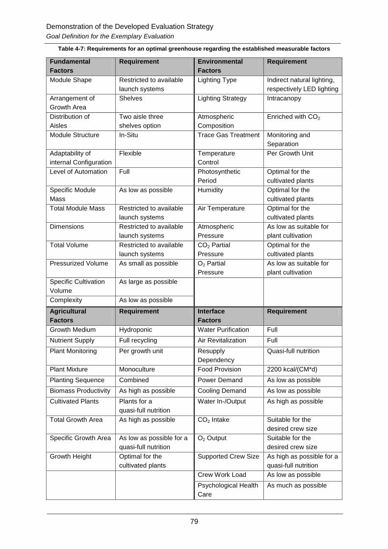
Demonstration of the Developed Evaluation Strategy
Goal Definition for the Exemplary Evaluation
79
Table 4-7: Requirements for an optimal greenhouse regarding the established measurable factors
Fundamental
Factors
Requirement Environmental
Factors
Requirement
Module Shape Restricted to available
launch systems
Lighting Type Indirect natural lighting,
respectively LED lighting
Arrangement of
Growth Area
Shelves Lighting Strategy Intracanopy
Distribution of
Aisles
Two aisle three
shelves option
Atmospheric
Composition
Enriched with CO2
Module Structure In-Situ Trace Gas Treatment Monitoring and
Separation
Adaptability of
internal Configuration
Flexible Temperature
Control
Per Growth Unit
Level of Automation Full Photosynthetic
Period
Optimal for the
cultivated plants
Specific Module
Mass
As low as possible Humidity Optimal for the
cultivated plants
Total Module Mass Restricted to available
launch systems
Air Temperature Optimal for the
cultivated plants
Dimensions Restricted to available
launch systems
Atmospheric
Pressure
As low as suitable for
plant cultivation
Total Volume Restricted to available
launch systems
CO2 Partial
Pressure
Optimal for the
cultivated plants
Pressurized Volume As small as possible O2 Partial
Pressure
As low as suitable for
plant cultivation
Specific Cultivation
Volume
As large as possible
Complexity As low as possible
Agricultural
Factors
Requirement Interface
Factors
Requirement
Growth Medium Hydroponic Water Purification Full
Nutrient Supply Full recycling Air Revitalization Full
Plant Monitoring Per growth unit Resupply
Dependency
Quasi-full nutrition
Plant Mixture Monoculture Food Provision 2200 kcal/(CM*d)
Planting Sequence Combined Power Demand As low as possible
Biomass Productivity As high as possible Cooling Demand As low as possible
Cultivated Plants Plants for a
quasi-full nutrition
Water In-/Output As high as possible
Total Growth Area As high as possible CO2 Intake Suitable for the
desired crew size
Specific Growth Area As low as possible for a
quasi-full nutrition
O2 Output Suitable for the
desired crew size
Growth Height Optimal for the
cultivated plants
Supported Crew Size As high as possible for a
quasi-full nutrition
Crew Work Load As low as possible
Psychological Health
Care
As much as possible
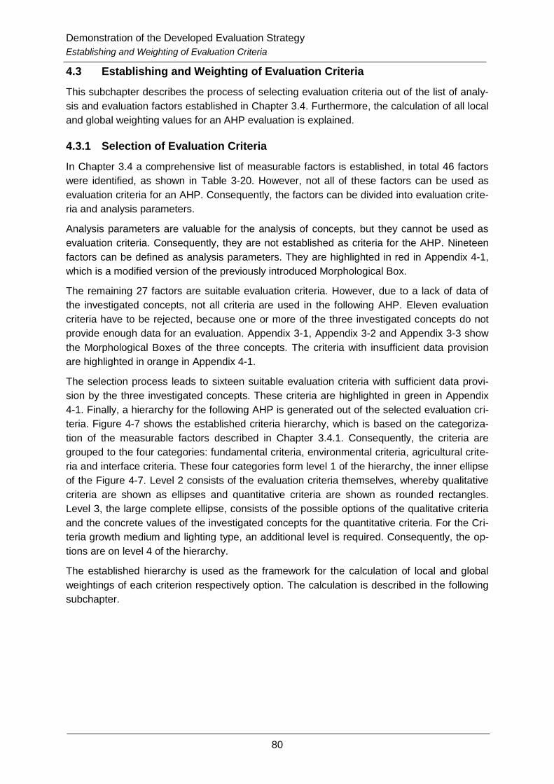
Demonstration of the Developed Evaluation Strategy
Establishing and Weighting of Evaluation Criteria
80
4.3 Establishing and Weighting of Evaluation Criteria
This subchapter describes the process of selecting evaluation criteria out of the list of analy-
sis and evaluation factors established in Chapter 3.4. Furthermore, the calculation of all local
and global weighting values for an AHP evaluation is explained.
4.3.1 Selection of Evaluation Criteria
In Chapter 3.4 a comprehensive list of measurable factors is established, in total 46 factors
were identified, as shown in Table 3-20. However, not all of these factors can be used as
evaluation criteria for an AHP. Consequently, the factors can be divided into evaluation crite-
ria and analysis parameters.
Analysis parameters are valuable for the analysis of concepts, but they cannot be used as
evaluation criteria. Consequently, they are not established as criteria for the AHP. Nineteen
factors can be defined as analysis parameters. They are highlighted in red in Appendix 4-1,
which is a modified version of the previously introduced Morphological Box.
The remaining 27 factors are suitable evaluation criteria. However, due to a lack of data of
the investigated concepts, not all criteria are used in the following AHP. Eleven evaluation
criteria have to be rejected, because one or more of the three investigated concepts do not
provide enough data for an evaluation. Appendix 3-1, Appendix 3-2 and Appendix 3-3 show
the Morphological Boxes of the three concepts. The criteria with insufficient data provision
are highlighted in orange in Appendix 4-1.
The selection process leads to sixteen suitable evaluation criteria with sufficient data provi-
sion by the three investigated concepts. These criteria are highlighted in green in Appendix
4-1. Finally, a hierarchy for the following AHP is generated out of the selected evaluation cri-
teria. Figure 4-7 shows the established criteria hierarchy, which is based on the categoriza-
tion of the measurable factors described in Chapter 3.4.1. Consequently, the criteria are
grouped to the four categories: fundamental criteria, environmental criteria, agricultural crite-
ria and interface criteria. These four categories form level 1 of the hierarchy, the inner ellipse
of the Figure 4-7. Level 2 consists of the evaluation criteria themselves, whereby qualitative
criteria are shown as ellipses and quantitative criteria are shown as rounded rectangles.
Level 3, the large complete ellipse, consists of the possible options of the qualitative criteria
and the concrete values of the investigated concepts for the quantitative criteria. For the Cri-
teria growth medium and lighting type, an additional level is required. Consequently, the op-
tions are on level 4 of the hierarchy.
The established hierarchy is used as the framework for the calculation of local and global
weightings of each criterion respectively option. The calculation is described in the following
subchapter.

Figure 4-7: Hierarchy of the selected evaluation criteria (level 1 to level 4, from the inside to the outside)
81
De
mo
nstra
tion
of th
e D
evelo
pe
d E
va
luatio
n S
trate
gy
Esta
blis
hin
g a
nd W
eig
htin
g o
f Eva
luatio
n C
riteria

Demonstration of the Developed Evaluation Strategy
Establishing and Weighting of Evaluation Criteria
82
4.3.2 Calculation of Local and Global Weightings
The calculation of local and global weightings for the selected evaluation criteria is based on
the equations presented in Chapter 3.3.2. An Excel file is generated for the calculation which
covers all pairwise comparisons, the calculation of weightings and the consistency check.
Furthermore, the evaluation of the three selected greenhouse module concepts is also in-
cluded in the Excel file. This subchapter shows an exemplary calculation and presents all
resulting values for the local and global weighting of the selected criteria.
The weighting of the criteria is based on the goal of the demonstration of the developed
analysis and evaluation methodology. The detailed goal definition is described in Chapter
4.2.
The pairwise comparisons are generally based on scientific background. However, the sub-
jective opinion of the analyst affects the rating of the comparisons. Consequently, a small
group of greenhouse experts working on the greenhouse project of the Institute of Space
Systems of the German Aerospace Center (DLR) in Bremen was formed for the rating of the
pairwise comparisons. The use of a small group of experts during an AHP is a suitable
method to reduce the bias during the establishing of the pairwise comparisons. The group of
experts consisted of the author of this thesis (graduate student in aerospace engineering),
the DLR greenhouse project leader, a graduate student of biology and two other aerospace
engineering graduate students. The final values for the pairwise comparisons are the results
of negotiations and discussions between the five group members.
In the following the calculation of the local weightings of the four criteria categories on level 1
of the hierarchy is shown. The calculation process is same for all local weightings. Conse-
quently, the shown calculation stands representatively for all local weighting calculations.
Level 1 of the AHP hierarchy consists of the four elements:
- Fundamental Criteria (FC),
- Environmental Criteria (EC),
- Agricultural Criteria (AC),
- Interface Criteria (IC).
The weighting calculation starts with the pairwise comparison of the four elements. There-
fore, each element is compared one by one to each of the other elements. For the compari-
son the rating system shown in Table 3-3 is used. The result of the pairwise comparison is
the comparison matrix. Table 4-8 shows the comparison matrix for the calculation of local
weightings for level 1 of the hierarchy. Thereby, the values of the pairwise comparisons are
inserted in the lower left part of the matrix, while the upper right half is the reciprocal of the
lower left half. Consequently, environmental criteria have a strong importance over funda-
mental criteria, or the importance of environmental criteria is four times higher compared to
fundamental criteria. Agricultural criteria have a moderate importance over fundamental crite-
ria, but they are only half important as environmental criteria. The importance of interface cri-
teria compared to fundamental, environmental and agricultural criteria is one third, one ninth
and one fifth.

Demonstration of the Developed Evaluation Strategy
Establishing and Weighting of Evaluation Criteria
83
Table 4-8: Comparison matrix for the calculation of local weightings of hierarchy level 1
Comparison Matrix
FC EC AC IC
FC 1 0.250 0.333 3.000
EC 4.000 1 2.000 9.000
AC 3.000 0.500 1 5.000
IC 0.333 0.111 0.200 1
Σ Column 8.333 1.861 3.533 18.000
The values of the pairwise comparisons are then normalized by the sum of their related col-
umn. Afterwards, the normalized values are summed up row by row. The result is the normal-
ization matrix shown in Table 4-9. Finally, the local weighting is calculated by dividing the
sum of each row by the size of the matrix. In the shown example the matrix has a size of
four.
Table 4-9: Normalization matrix and local weightings of hierarchy level 1
Normalization
Weighting
FC EC AC IC Σ Row w
FC 0.120 0.134 0.094 0.167 0.515 0.129
EC 0.480 0.537 0.566 0.500 2.083 0.521
AC 0.360 0.269 0.283 0.278 1.189 0.297
IC 0.040 0.060 0.057 0.056 0.212 0.053
Σ Column 1.000 1.000 1.000 1.000 4.000 1.000
The exact local weightings for the four elements on level 1 of the hierarchy are:
- Fundamental Criteria = 0.12883,
- Environmental Criteria = 0.52084,
- Agricultural Criteria = 0.29736,
- Interface Criteria = 0.05297.
Consequently, the selected environmental criteria have the highest impact on the total
weighting score of the investigated concepts, followed by the agricultural, the fundamental
and the interface criteria.
The calculation of the local weightings is followed by the consistency check, in which the
consistency of the pairwise comparisons is investigated. Therefore, the mean matrix is gen-
erated to calculate the Eigenvalue of each element of the matrix. Table 4-10 shows the mean
matrix and the related Eigenvalues for each element.
The Eigenvalues are part of the calculation of the consistency relationship (CR), as de-
scribed in Chapter 3.2. The CR value for the local weighting calculations of hierarchy level 1
is 0.014. The boundary value for consistency is 0.1, a CR smaller than the boundary value
leads to a consistent pairwise comparison. Consequently, the pairwise comparisons of level
1 are consistent and therefore, the local weightings are reliable.
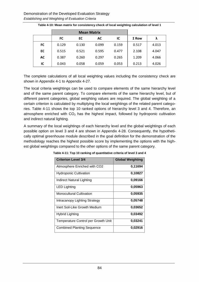
Demonstration of the Developed Evaluation Strategy
Establishing and Weighting of Evaluation Criteria
84
Table 4-10: Mean matrix for consistency check of local weighting calculation of level 1
Mean Matrix
FC EC AC IC Σ Row λ
FC 0.129 0.130 0.099 0.159 0.517 4.013
EC 0.515 0.521 0.595 0.477 2.108 4.047
AC 0.387 0.260 0.297 0.265 1.209 4.066
IC 0.043 0.058 0.059 0.053 0.213 4.026
The complete calculations of all local weighting values including the consistency check are
shown in Appendix 4-1 to Appendix 4-27.
The local criteria weightings can be used to compare elements of the same hierarchy level
and of the same parent category. To compare elements of the same hierarchy level, but of
different parent categories, global weighting values are required. The global weighting of a
certain criterion is calculated by multiplying the local weightings of the related parent catego-
ries. Table 4-11 shows the top 10 ranked options of hierarchy level 3 and 4. Therefore, an
atmosphere enriched with CO2 has the highest impact, followed by hydroponic cultivation
and indirect natural lighting.
A summary of the local weightings of each hierarchy level and the global weightings of each
possible option on level 3 and 4 are shown in Appendix 4-28. Consequently, the hypotheti-
cally optimal greenhouse module described in the goal definition for the demonstration of the
methodology reaches the highest possible score by implementing the options with the high-
est global weightings compared to the other options of the same parent category.
Table 4-11: Top 10 ranking of quantitative criteria of level 3 and 4
Criterion Level 3/4 Global Weighting
Atmosphere Enriched with CO2 0,11694
Hydroponic Cultivation 0,10827
Indirect Natural Lighting 0,09166
LED Lighting 0,05963
Monocultural Cultivation 0,05935
Intracanopy Lighting Strategy 0,05748
Inert Soil-Like Growth Medium 0,03652
Hybrid Lighting 0,03492
Temperature Control per Growth Unit 0,03241
Combined Planting Sequence 0,02916
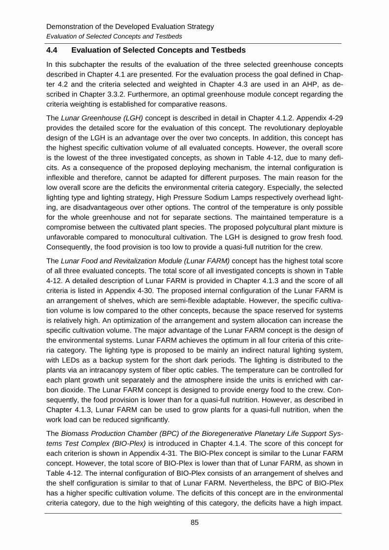
Demonstration of the Developed Evaluation Strategy
Evaluation of Selected Concepts and Testbeds
85
4.4 Evaluation of Selected Concepts and Testbeds
In this subchapter the results of the evaluation of the three selected greenhouse concepts
described in Chapter 4.1 are presented. For the evaluation process the goal defined in Chap-
ter 4.2 and the criteria selected and weighted in Chapter 4.3 are used in an AHP, as de-
scribed in Chapter 3.3.2. Furthermore, an optimal greenhouse module concept regarding the
criteria weighting is established for comparative reasons.
The Lunar Greenhouse (LGH) concept is described in detail in Chapter 4.1.2. Appendix 4-29
provides the detailed score for the evaluation of this concept. The revolutionary deployable
design of the LGH is an advantage over the over two concepts. In addition, this concept has
the highest specific cultivation volume of all evaluated concepts. However, the overall score
is the lowest of the three investigated concepts, as shown in Table 4-12, due to many defi-
cits. As a consequence of the proposed deploying mechanism, the internal configuration is
inflexible and therefore, cannot be adapted for different purposes. The main reason for the
low overall score are the deficits the environmental criteria category. Especially, the selected
lighting type and lighting strategy, High Pressure Sodium Lamps respectively overhead light-
ing, are disadvantageous over other options. The control of the temperature is only possible
for the whole greenhouse and not for separate sections. The maintained temperature is a
compromise between the cultivated plant species. The proposed polycultural plant mixture is
unfavorable compared to monocultural cultivation. The LGH is designed to grow fresh food.
Consequently, the food provision is too low to provide a quasi-full nutrition for the crew.
The Lunar Food and Revitalization Module (Lunar FARM) concept has the highest total score
of all three evaluated concepts. The total score of all investigated concepts is shown in Table
4-12. A detailed description of Lunar FARM is provided in Chapter 4.1.3 and the score of all
criteria is listed in Appendix 4-30. The proposed internal configuration of the Lunar FARM is
an arrangement of shelves, which are semi-flexible adaptable. However, the specific cultiva-
tion volume is low compared to the other concepts, because the space reserved for systems
is relatively high. An optimization of the arrangement and system allocation can increase the
specific cultivation volume. The major advantage of the Lunar FARM concept is the design of
the environmental systems. Lunar FARM achieves the optimum in all four criteria of this crite-
ria category. The lighting type is proposed to be mainly an indirect natural lighting system,
with LEDs as a backup system for the short dark periods. The lighting is distributed to the
plants via an intracanopy system of fiber optic cables. The temperature can be controlled for
each plant growth unit separately and the atmosphere inside the units is enriched with car-
bon dioxide. The Lunar FARM concept is designed to provide energy food to the crew. Con-
sequently, the food provision is lower than for a quasi-full nutrition. However, as described in
Chapter 4.1.3, Lunar FARM can be used to grow plants for a quasi-full nutrition, when the
work load can be reduced significantly.
The Biomass Production Chamber (BPC) of the Bioregenerative Planetary Life Support Sys-
tems Test Complex (BIO-Plex) is introduced in Chapter 4.1.4. The score of this concept for
each criterion is shown in Appendix 4-31. The BIO-Plex concept is similar to the Lunar FARM
concept. However, the total score of BIO-Plex is lower than that of Lunar FARM, as shown in
Table 4-12. The internal configuration of BIO-Plex consists of an arrangement of shelves and
the shelf configuration is similar to that of Lunar FARM. Nevertheless, the BPC of BIO-Plex
has a higher specific cultivation volume. The deficits of this concept are in the environmental
criteria category, due to the high weighting of this category, the deficits have a high impact.
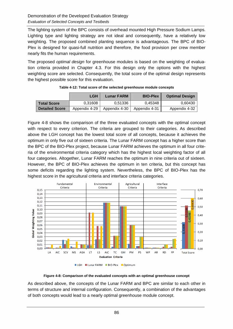
Demonstration of the Developed Evaluation Strategy
Evaluation of Selected Concepts and Testbeds
86
The lighting system of the BPC consists of overhead mounted High Pressure Sodium Lamps.
Lighting type and lighting strategy are not ideal and consequently, have a relatively low
weighting. The proposed combined planting sequence is advantageous. The BPC of BIO-
Plex is designed for quasi-full nutrition and therefore, the food provision per crew member
nearly fits the human requirements.
The proposed optimal design for greenhouse modules is based on the weighting of evalua-
tion criteria provided in Chapter 4.3. For this design only the options with the highest
weighting score are selected. Consequently, the total score of the optimal design represents
the highest possible score for this evaluation.
Table 4-12: Total score of the selected greenhouse module concepts
LGH Lunar FARM BIO-Plex Optimal Design
Total Score 0,31608 0,51336 0,45348 0,60430
Detailed Score Appendix 4-29 Appendix 4-30 Appendix 4-31 Appendix 4-32
Figure 4-8 shows the comparison of the three evaluated concepts with the optimal concept
with respect to every criterion. The criteria are grouped to their categories. As described
above the LGH concept has the lowest total score of all concepts, because it achieves the
optimum in only five out of sixteen criteria. The Lunar FARM concept has a higher score than
the BPC of the BIO-Plex project, because Lunar FARM achieves the optimum in all four crite-
ria of the environmental criteria category which has the highest local weighting factor of all
four categories. Altogether, Lunar FARM reaches the optimum in nine criteria out of sixteen.
However, the BPC of BIO-Plex achieves the optimum in ten criteria, but this concept has
some deficits regarding the lighting system. Nevertheless, the BPC of BIO-Plex has the
highest score in the agricultural criteria and interface criteria categories.
Figure 4-8: Comparison of the evaluated concepts with an optimal greenhouse concept
As described above, the concepts of the Lunar FARM and BPC are similar to each other in
terms of structure and internal configuration. Consequently, a combination of the advantages
of both concepts would lead to a nearly optimal greenhouse module concept.
Demonstration of the Developed Evaluation Strategy
Summary
87
4.5 Summary
Chapter 4 demonstrates the previously developed analysis and evaluation methodology.
Therefore, a survey on existing greenhouse module concepts and test facilities is executed in
the first subchapter. Out of the provided list of greenhouse modules, three concepts were
selected for further investigation. All three greenhouses are analyzed in detail in the first sub-
chapter.
The second subchapter defines the goal of the exemplary evaluation. A hypothetically opti-
mal greenhouse module is established for the demonstration of the methodology. Therefore,
the best options of the previously established evaluation factors are combined. The proper-
ties of the optimal greenhouse module are shown.
The third subchapter describes the selection process of the evaluation criteria. Depending on
the available data of the selected concepts and the characteristics of the established factors,
the evaluation criteria are selected. A hierarchy based on the factor categorization is created
for the AHP evaluation. Furthermore, the local and global weightings for all elements of the
hierarchy are calculated and checked on consistency. The calculation of the weightings is
based on the previously defined goal of the evaluation. The values are calculated by the
equations of the AHP described in Chapter 3.3.2 and are the results of the pairwise compari-
sons of the elements of the hierarchy.
The fourth subchapter utilizes the established criteria weighting for the evaluation of the three
selected greenhouse module concepts. The Lunar Greenhouse (LGH) achieves the lowest
score due to deficits regarding the environmental criteria. The Biomass Production Chamber
(BPC) of the BIO-Plex facility has a high score in the agricultural criteria category. However,
due to minor deficits in the environmental criteria category, especially the lighting system, the
BPC of BIO-Plex achieves only the second highest score of all three concepts. The green-
house module concept with the highest total score is the Lunar Food and Revitalization Mod-
ule (Lunar FARM). Lunar FARM reaches the optimum in all subcriteria of the environmental
criteria category, which has the highest influence. However, even the Lunar FARM concept
has deficits compared to an optimal concept, especially, in the agricultural criteria category.
Finally, a combination of the advantages of Lunar FARM and the BPC of BIO-Plex could
achieve a score similar to the hypothetically optimal greenhouse module design.

Discussion
88
5 Discussion
Terrestrial human isolation test beds like the Japanese Closed Ecology Experiment Facilities
and the Russian BIOS-3 demonstrated the possibility of providing food with greenhouse
modules to humans in a closed environment. Furthermore, the air revitalization and water
purification with the use of the plants inside the greenhouse module worked well. Green-
house modules as part of ECLSS of crewed spacecraft or habitats are necessary for future
long term or even permanent missions to Moon and Mars.
Unfortunately, the prospects for utilization of greenhouse modules in a planetary mission in
the near future are, at this stage, minimal. Neither NASA nor ESA have concrete plans for
crewed long duration missions to planetary bodies in the near future. However, the today’s
research related to greenhouse modules is necessary, because of the not well understood
relation between plants, humans and environmental conditions in closed ecosystems. This
thesis lays a profound scientific background for the ongoing research activities at the DLR
Bremen.
This thesis provides a comprehensive list of measurable factors. However, future research-
ers might think about adding their own factors, which is feasible due to the general nature of
the selected analysis and evaluation methods. Consequently, the proposed methodology can
be adapted to future evaluations by the analysts. This makes the analysis and evaluation
strategy to a favorable tool for the investigation of developed greenhouse modules designs.
The selected evaluation criteria can be freely adapted to fit to the goals of future investiga-
tions of greenhouses. In addition the possibility of recalculating the criteria weighting exists
and could be necessary for other evaluation goals. The generated Excel file can be used as
tool for future calculations of criteria weightings.
However, for the defined goal of the exemplary evaluation of the selected greenhouses, the
criteria weighting is reliable. This reliability can be guaranteed, because of the negotiation of
a group of greenhouse researchers. The weightings himself are checked on consistency and
no inconsistent weighting could be identified. The greenhouse concept with the highest
score, the Lunar FARM, has a sophisticated design and the simulations executed during the
design of this concept provide a good data source. Nevertheless, the evaluation showed, that
even the Lunar FARM concept cannot match with the established hypothetically greenhouse
design.
The relations between the measurable factors are not investigated during this thesis. Espe-
cially, the strong dependencies between the lighting, the air temperature, humidity, CO2 level
and biomass production have to be investigated in future researches. The dependencies be-
tween different factors can affect the criteria weighting. The implementation of the results of a
detailed analysis of the relations can improve the reliability of the proposed analysis and
evaluation methodology.
The adaptability and the generality of the developed strategy allow the use in future investi-
gation of the DLR research efforts in the niche field of greenhouse modules for space appli-
cations. The outcome can be used for future research activities in the system design of
greenhouse modules, laboratories and test facilities.
Summary
89
6 Summary
The topic of this thesis was the system analysis and evaluation of greenhouse modules for
planetary habitats. A survey on existing plant growth chambers, greenhouse modules and
terrestrial test facilities had been executed to accomplish a list of concepts. For the analysis
and evaluation of greenhouse modules a methodology had been developed. Therefore,
measurable factors concerning the performance, agricultural properties and in-/output of
greenhouse modules had been defined. The developed strategy had been executed on se-
lected greenhouse module concepts to demonstrate the workability and reliability.
Chapter 2 of present thesis provides a profound scientific background related to environmen-
tal conditions, human requirements, ECLSS, food provision in crewed spacecraft and green-
house module subsystems.
The first subchapter of Chapter 3 explains the developed analysis and evaluation methodol-
ogy. The strategy consists of a four step approach, starting with the data acquisition, followed
by the system analysis, the evaluation and the discussion. The second subchapter describes
the proposed system analysis method, the Morphological Analysis, which is a suitable analy-
sis method to structure problems. The third subchapter explains the two proposed evaluation
methods, the Equivalent System Mass (ESM) approach and the Analytical Hierarchy Process
(AHP). Finally, the AHP was selected, due to the advantage of using qualitative criteria. The
fourth subchapter defines the investigated measurable factors. A factor categorization had
been established and detailed descriptions for every factor were provided.
Chapter 4 shows an exemplary evaluation of preselected greenhouse modules. This chapter
starts with a survey on existing plant growth chambers, greenhouse module concepts and
terrestrial test facilities. The Lunar Greenhouse (LGH), the Lunar Food and Revitalization
Module (Lunar FARM) and the Biomass Production Chamber (BPC) of the BIO-Plex facility
were selected for further investigation and evaluation. The second subchapter defines the
goal of the evaluation. In the third subchapter, evaluation criteria are shown and the
weighting calculations of each criterion based on the AHP equations are depicted. The fourth
subchapter described the results of the evaluation.
Chapter 5 discusses the outcomes of this thesis. As demonstrated the proposed analysis
and evaluation strategy is suitable and reliable method for the investigation and comparison
of existing greenhouse module concepts. Furthermore, the established measurable factors
and evaluation criteria hierarchies can be expanded if necessary for future evaluations. In
addition to the analysis and evaluation the defined factors can be used in the design phase
of future greenhouse modules and can assists the designing engineer during trade studies of
different systems.

X
List of References
[1] Peter Eckart, "The Extraterrestrial Environment," in Spaceflight Life Support and
Biospherics.: Microcosm Press, Kluwer Academic Publishers, 1996, ch. III.
[2] Erik Gregersen, "The Moon," in The Inner Solar System: The Sun, Mercury, Venus,
Earth, and Mars.: Britannica Educational Publishing, 2010, ch. 6.
[3] Erik Gregersen, "Mars," in The Inner Solar System: The Sun, Mercury, Venus, Earth,
and Mars.: Britannica Educational Publishing, 2010, ch. 8.
[4] Erik Gregersen, "Earth," in The Inner Solar System: The Sun, Mercury, Venus, Earth,
and Mars.: Britannica Educational Publishing, 2010, ch. 5.
[5] NASA, "NASA space flight human-system standard - Volume 2: human factors,
habitability, and environmental health," NASA, NASA-STD-3001, Volume 2, 2011.
[6] Peter Eckart, "Fundamentals of Life Support Systems," in Spaceflight Life Support an
Biospherics.: Microcosm Press, Kluwer Academic Publishers, 1996, ch. IV.
[7] Paul O. Wieland, "ECLS - Purpose and functions," in Designing for human presence in
space - An introduction to environmental control and life support systems.: NASA, 1994,
ch. 2.
[8] NASA, "Advanced life support requirements document ," NASA, CTSD-ADV-245C,
2003.
[9] Ernst Messerschmid and Reinhold Bertrand, "Environmental control and life support
system," in Space stations - systems and utilization.: Springer, 1999, ch. 4.
[10] Peter Eckart, "Physico-Chemical Life Support Subsystems," in Spaceflight Life Support
and Biospherics.: Microcosm Press, Kluwer Academic Publishers, 1996, ch. V.
[11] Paul O. Wieland, "Beyond low earth orbit - The challenge of remote ECLS," in Designing
for human presence in space - An introduction to environmental control and life support
systems.: NASA, 1994, ch. 7.
[12] Sandra Häuplik-Meusburger, "Food," in Architecture for Astronauts - An Activity-based
Approach.: Springer, 2011, ch. 6, pp. 202-229.
[13] Michele Perchonok. (2012, May) Habitability and Environmental Factors - Advanced
Food Technology Project. [Online].
http://www.nasa.gov/centers/johnson/slsd/about/divisions/hefd/project/advanced-
foods.html
[14] Thomas P. Sarafin, Peter G. Doukas, James R. McCandless, and William R. Britton,
"Structures and mechanisms," in Space mission analysis and design.: Microcosm Press
& Kluwer Academic Publishers, 2005, ch. 11.6.
[15] Joseph K. McDermott, "Power," in Space mission analysis and design.: Microcosm
Press & Kluwer Academic Publishers, 2005, ch. 11.4.

XI
[16] Richard T. Berget, "Command and data handling," in Space Mission Analysis and
Design.: Microcosm Press & Kluwer Academic Publishers, 2005, ch. 11.3.
[17] David G. Gilmore, Brian E. Hardt, Robert C. Prager, Eric W. Grob, and Wes Ousley,
"Thermal," in Space mission analysis and design.: Microcosm Press & Kluwer Academic
Publishers, 2005, ch. 11.5.
[18] Robert U. Ayers, "Morphological Analysis," in Technological Forecasting and Long-
Range Planning.: McGraw-Hill Book Company, 1969, ch. 5, p. 72.
[19] Robert U. Ayres, "Morphological Analysis," in Technological Forecasting and Long-
Range Planning.: McGraw-Hill Book Company, 1969, ch. 5.
[20] Jerome C. Glenn and Theodore J. Gordon, "Relevance tree and morphological analysis
- v2.0," in Futures research methodology.: American Council for the United Nations
University - The Millenium Project, 2007, ch. 12.
[21] Julie A. Levri et al., "Advanced Life Support Equivalent System Mass Guidelines
Document," NASA, Ames Research Center, NASA/TM-2003-212278, 2003.
[22] Kristin W. Stafford et al., "Advanced Life Support Systems Integration, Modeling, and
Analysis Reference Missions Document," NASA, Lyndon B. Johnson Space Center,
CTSD-ADV-383, 2001.
[23] Anthony J. Hanford and Michael K. Ewert, "Advanced Life Support Baseline Values and
Assumptions Document," NASA, Lyndon B. Johnson Space Center, NASA/CR—2004–
208941, 2004.
[24] Dieter Brinkmeyer and Rolf A. E. Müller, "Entscheidungsunterstützung mit dem AHP,"
Zeitschrift für Agrarinformatik, pp. 82-92, May 1994.
[25] R. W. Saaty, "The analytic hierarchy process - What it is and how it is used,"
Mathematical Moddeling, vol. 9, no. 3-5, pp. 161-176, 1987.
[26] Thomas L. Saaty, "Decision making with the analytic hierarchy process," Int. J. Services
Sciences, vol. 1, no. 1, pp. 83-98, 2008.
[27] Oliver Meixner and Rainer Haas, Computergestützte Entscheidungsfindung. Expert
Choice und AHP - innovative Werkzeuge zur Lösung komplexer Probleme, 1st ed.:
Redline Wirtschaft, 2002.
[28] Marc M. Cohen and Haym Benaroya, "Lunar-base structures," in Out of this world - The
new field of space architecture.: American Institute of Aeronautics and Astronautics,
2009, ch. 15, pp. 179-204.
[29] Yu. A. Berkovich et al., "Vegetable production facility as a part of a closed life support
system in a Russian Martian space flight scenario," Advances in Space Research, vol.
44, pp. 170-176, March 2009.
[30] Omega Garden International. (2012, March) Omega Garden. [Online].
http://www.omegagarden.com/index.php?content_id=1521#greenhouses

XII
[31] Claudio Finetto, Cesare Lobascio, and Alessandro Rapisarda, "Conept of a lunar FARM:
Food and revitalization module," Acta Astronautica, vol. 66, pp. 1329-1340, 2010.
[32] Daniel J. Barta, Juan M. Castillo, and Russ E. Fortson, "The biomass production system
for the bioregenartive planetary life support systems test complex: Preliminary designs
and considerations," 29th International Conference on Environmental Systems, Denver,
SAE Technical Papers Series 1999-01-2188, July 1999.
[33] T. W. Tibbitts, "Plant considerations for Lunar base agriculture," in Lunar base griculture
- Soils for plant growth.: American Society of Agronomy, Crop Science Society of
America, Soil Science Society of America, 1989, ch. 17, pp. 237-243.
[34] John C. Sager and J. Craig Mc Farlane, "Radiation," in Plant Growth Chamber
Handbook.: Iowa Agriculture and Home Economics Experiment Station, 1997, ch. 1, pp.
1-29.
[35] D. T. Krizek, R. M. Mirecki, and W. A. Bailey, "Uniformity of photosynthetic photon flux
and growth of 'poinsett' cucumber plants under metal halide and microwave-powered
sulfur lamps," Biotronics, vol. 27, pp. 81-92, 1998.
[36] Klaus Streubel, "Visible light-emitting diodes," in Handbook of Optoelectronics.: Taylor &
Francis Group, 2006, ch. B1.1, pp. 329-384.
[37] Gioia D. Massa, Jeffrey C. Emmerich, Robert C. Morrow, C. Mike Bourger, and Cary A.
Mitchell, "Plant-growth lighting for space life support: A review," Gravitational and Space
Biology, vol. 19, no. 2, pp. 19-30, August 2006.
[38] M. A. Dixon, B. Grodzinski, R. Côté, and M. Stasiak, "Sealed environment chamber for
canopy light interception and trace hydrocarbon analysis," Advances in space research,
vol. 24, no. 3, pp. 271-280, 1999.
[39] Alan Drysdale, Takashi Nakamura, Neil Yorio, John Sager, and Ray Wheeler, "Use of
sunlight for plant lighting in a bioregenerative life aupport system - Equivalent system
mass calculations," Advances in space research, vol. 42, pp. 1929-1943, 2008.
[40] Mary M. Peet and Donald T. Krizek, "Carbon dioxide," in Plant Growth Chamber
Handbook.: Iowa Agriculture and Home Economics Experiment Station, 1997, ch. 4, pp.
65-79.
[41] Theodore W. Tibbitts, "Air Contaminants," in Plant Growth Chamber Handbook.: Iowa
Agriculture and Home Economics Experiment Stat, 1997, ch. 5, pp. 81-87.
[42] Peter R. Hicklenton and Royal D. Heins, "Temperature," in Plant Growth Chamber
Handbook.: Iowa Agriculture and Home Economics Experiment Station, 1997, ch. 2, pp.
31-42.
[43] T. W. Tibbitts and D. L. Henninger, "Food production in space: Challenges and
perspectives," in Plant production in closed ecosystems.: Kluwer Academic Publishers,
1996, pp. 189-203.
XIII
[44] E. Goto, "Environmental control for plant production in space CELSS," in Plant
production in closed ecosystems.: Kluwer Academic Publishers, 1996, ch. B, pp. 279-
296.
[45] Peter Eckart, "Bioregenerative Life Support Concepts," in Spaceflight Life Support and
Biospherics.: Microcosm Press, Kluwer Academic Publishers, 1996, ch. VI.
[46] Douglas W. Ming, "Manufactured Soils for Plant Growh at a Lunar Base," in Lunar Base
Agriculture: Soils for Plant Growth.: American Society of Agronomy, Crop Science
Society of America, Soil Science Society of America, 1989, ch. 7, pp. 93-105.
[47] P. A. Helmke and R. B. Corey, "Physical and Chemical Considerations for the
Development of Lunar Derived Soils," in Lunar Base Agriculture: Soils for Plant Growth.:
American Society of Agronomy, Crop Science Society of America, Soil Science Society
of America, 1989, ch. 15, pp. 193-212.
[48] Bruce G. Bugbee and Frank B. Salisbury, "Controlled Environment Crop Production:
Hydroponic vs. Lunar Regolith," in Lunar Base Agriculture: Soils for Plant Growth.:
American Society of Agronomy, Crop Science Society of America, Soil Science Society
of America, 1989, ch. 8, pp. 107-129.
[49] Raymond M. Wheeler, "Expert opinion concerning greenhouse modules," NASA,
Personal Communication 12.02.2012.
[50] Wolfgang Franke, Reinhard Lieberei, and Christoph Reisdorff, "Nahrungspflanzen," in
Nutzpflanzenkunde: Nutzbare Gewächse der gemässigten Breiten, Subtropen und
Tropen, 7th ed.: Thieme, 2007, ch. 4, pp. 67-356.
[51] Sandra Häuplik-Meusburger, Regina Peldszus, and Verena Holzgethan, "Greenhouse
design integratipn benefits for extended spaceflight," Acta Astronautica, vol. 68, pp. 85-
90, 2011.
[52] Robert A. Aldrich and John W. Bartok Jr., "Greenhouse planning," in Greenhouse
engineering, 3rd ed.: Natural Resource, Agriculture, and Engineering Service, 1994, ch.
1, p. 1.
[53] A. Hoehn et al., "Mass transport in a spaceflight plant growth chamber," 28th
International Conference on Environmental Systems, Danvers, SAE Technical Papers
Series 981553, 1998.
[54] S. Guo et al., "Development of a CELSS Experimental Facility," Advances in Space
Research, vol. 41, pp. 725-729, September 2008.
[55] R. M. Wheeler et al., "NASA's biomass production chamber: A testbed for
bioregenerative life support studies," Advances in Space Research, vol. 18, no. 4/5, pp.
215-224, 1996.
[56] W. M. Knott, "The breadboard project: A functioning CELSS plant growth system,"
Advances in Space Research, vol. 12, no. 5, pp. 45-52, 1992.

XIV
[57] R. M. Wheeler et al., "Crop production for advanced life support systems," NASA,
Kennedy Space Center, Technical Report NASA/TM–2003-211184, 2003.
[58] Phil Sadler, Gene Giacomelli, Roberto Furfaro, Randy Patterson, and Murat Kacira,
"Prototype BLSS lunar greenhouse," University of Arizona, Paper 0148-7191, 2009.
[59] P. D. Sadler et al., "Bio-regenerative life support systems for space surface
applications," 41st International Conference on Environmental Systems, Portland,
Oregon, Paper AIAA 2011-5133, 2011.
[60] K. Nitta, K. Otsubo, and A. Ashida, "Integration test project of CEEF," Advances in
Space Research, vol. 26, no. 2, pp. 335-338, 2000.
[61] Keiji Nitta, "Basic design of closed ecology experiment facilities," Advances in Space
Research, vol. 24, no. 3, pp. 343-350, 1999.
[62] Keiji Nitta, "The mini-earth facility and present status of habitation experiment program,"
Advances in Space Research, vol. 35, pp. 1531-1538, March 2005.
[63] Tsuyoshi Masuda, "Food supplies for habitation experiments in an earth-based
advanced life support system," World of Food Science, vol. 2, pp. 1-10, October 2007.
[64] Y. Tako et al., "One-week habitation of two humans in an airtight facility with two goats
and 23 crops - Analysis of carbon, oxygen, and water circulation," Advances in Space
Research, vol. 41, pp. 714-724, 2008.
[65] Yasuhiro Tako et al., "CEEF: Closed ecology experiment facilities," Gravitational and
Space Biology, vol. 23, pp. 13-24, August 2010.
[66] I. I. Gitelson, G. M. Lisovsky, and R. D. MacElroy, "Experiments Testing Prolonged
Human Life in the Bios-3 Life Support System," in Manmade Closed Ecological
Systems.: Taylor & Francis Group, 2003, ch. 9, pp. 231-309.
[67] Frank B. Salisbury, Josef I. Gitelson, and Genry M. Lisovsky, "Bios-3: Siberian
experiments in bioregenerative life support," BioScience, vol. 47, no. 9, pp. 575-585,
October 1997.
[68] Josef I. Gitelson and Genry M. Lisovsky, "Creation of Closed Ecological Life Support
Systems: Results, Critical Problems and Potentials," Journal of Siberian Federal
University, vol. Biology 1, pp. 19-39, January 2008.
[69] J. I. Gitelson et al., "Long-term experiments on man's stay in biological life-support
system," Advances in Space Research, vol. 9, no. 8, pp. 65-71, 1989.
[70] J. D. Villarreal and T. O. Tri, "Bioregenerative Planetary Life Support Systems Test
Complex (BIO-Plex): Progress to Date," 31st International Conference on Environmental
Systems, Orlando, SAE Technical Papers Series 2001-01-2317, Juli 2001.
[71] M. Perchonok, E. Vittadini, B. E. Swango, M. E. Toerne, and L. Peterson,
"Bioregenerative planetary life support systems test complex (BIO-Plex) food processing
system; A dual task approach," NASA - JSC, Houston, Technical Report 2001-01-2321,
2001.
XV
[72] William F. Dempster, "Biosphere 2 engineering design," Ecological Engineering, vol. 13,
pp. 31-42, 1999.
[73] Bruno D. V. Marino and H. T. Odum, "Biosphere 2: Introduction and research progress,"
Ecological Engineering, vol. 13, pp. 3-14, 1999.
[74] Bruno D.V. Marino et al., "The agricultural biome of biosphere 2: Structure, composition
and function," Ecological Engineering, vol. 13, pp. 199-234, 1999.
[75] J. Poynter and D. Bearden, "Biosphere 2: A closed bioregenerative life support system,
An analog for long duration space missions," Plant Production in Closed Ecosystems,
pp. 263-277, 1997.
[76] Peter Eckart, "Biosphere 2 - Lessons Learned for Future CELSS Research," in
Spaceflight Life Support and Biospherics.: Microcosm Press, Kluwer Academic
Publishers, 1996, ch. VII.
[77] M. Bamsey et al., "Developing strategies for automated remote plant production
systems: Environmental control and monitoring of the arthur clarke mars greenhouse in
the canadian high arctic," Advances in Space Research, vol. 44, pp. 1367-1381, August
2009.
[78] M. Bamsey et al., "Canadian advanced life support spacities and future directions,"
Advances in Space Research, vol. 44, pp. 151-161, March 2009.
[79] Richard Giroux et al., "Greenhouses in extreme environments: The arthur clarke mars
greenhouse design and operation overview," Advances in Space Research, vol. 38, pp.
1248-1259, July 2006.
[80] Lane R. Patterson, Gene A. Giacomelli, and Phil D. Sadler, "Ressource and Production
Model for the South Pole Food Growth Chamber," 38th International Conference on
Environmental Systems, San Francisco, California, SAE Technical Paper Series 2008-
01-2011, July 2008.
[81] Claudio Finetto, Alessandro Rapisarda, Daniele Renzoni, Amir Sabbagh, and Cosimo
Sinesi, "Food an Revitalization Module (FARM) for Moon Human Exploration," 38th
International Conference on Environmental Systems, San Francisco, SAE Technical
Papers Series 2008-01-2014, 2008.
[82] Salvatore Cusumano, Alex Karl, Vincent Drevet-Cadet, and Alessandro Fimiani,
"PHOEBE - Permanent human moon exploration base," 2nd International Master Course
in Space Exploration and Development Systems (SEEDS), Executive Summary 2008.
[83] Ryan Ries et al., "RedThumb: A Mars Greenhouse Designfor the 2002 MarsPort
Engineering Design Student Competition," 33rd International Conference on
Environmental Systems, Vancouver, Canada, SAE Technical Paper Series 2003-01-
2676, July 2003.

XVI
Appendix 2-1: Recommended Macronutrient Daily Dietary Intake
The following table can be found in chapter 7 of reference [5].
Nutrients Daily Dietary Intake
Protein 0.8 g/kg
And ≤ 35 % of the total daily energy intake
And 2/3 of the amount in the form of animal protein and 1/3 in the form of
vegetable protein
Carbohydrate 50 – 55 % of the total daily energy intake
Fat 25 – 35 % of the total daily energy intake
Ω-6 fatty acids 14 g
Ω-3 fatty acids 1.1 – 1.6 g
Saturated fat < 7 % of the total energy intake
Trans fatty acids < 1 % of the total energy intake
Cholesterol < 300 mg/d
Fiber 10 – 14 g/4187 kJ
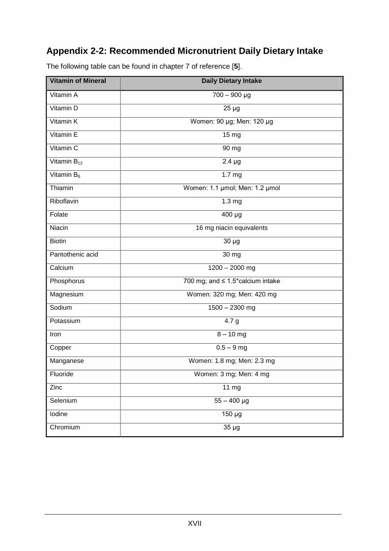
XVII
Appendix 2-2: Recommended Micronutrient Daily Dietary Intake
The following table can be found in chapter 7 of reference [5].
Vitamin of Mineral Daily Dietary Intake
Vitamin A 700 – 900 μg
Vitamin D 25 μg
Vitamin K Women: 90 μg; Men: 120 μg
Vitamin E 15 mg
Vitamin C 90 mg
Vitamin B12 2.4 μg
Vitamin B6 1.7 mg
Thiamin Women: 1.1 μmol; Men: 1.2 μmol
Riboflavin 1.3 mg
Folate 400 μg
Niacin 16 mg niacin equivalents
Biotin 30 μg
Pantothenic acid 30 mg
Calcium 1200 – 2000 mg
Phosphorus 700 mg; and ≤ 1.5*calcium intake
Magnesium Women: 320 mg; Men: 420 mg
Sodium 1500 – 2300 mg
Potassium 4.7 g
Iron 8 – 10 mg
Copper 0.5 – 9 mg
Manganese Women: 1.8 mg; Men: 2.3 mg
Fluoride Women: 3 mg; Men: 4 mg
Zinc 11 mg
Selenium 55 – 400 μg
Iodine 150 μg
Chromium 35 μg
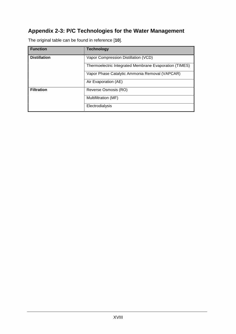
XVIII
Appendix 2-3: P/C Technologies for the Water Management
The original table can be found in reference [10].
Function Technology
Distillation Vapor Compression Distillation (VCD)
Thermoelectric Integrated Membrane Evaporation (TIMES)
Vapor Phase Catalytic Ammonia Removal (VAPCAR)
Air Evaporation (AE)
Filtration Reverse Osmosis (RO)
Multifiltration (MF)
Electrodialysis

XIX
Appendix 2-4: P/C Technologies for Air Revitalization
The original table can be found in reference [10].
Function Technology
Carbon Dioxide Removal 2-bed Molecular Sieve (2BMS)
4-bed Molecular Sieve (4BMS)
Electrochemical Depolarization Concentrator (EDC)
Solid Amine Water Desorption (SAWD)
Air Polarized Concentrators (APC)
Lithium Hydroxide (LiOH)
Carbon Dioxide Reduction Bosch Process
Sabatier Process
Advanced Carbon-Formation Reactor System
Carbon Dioxide Electrolysis
Superoxides
Artificial Gill
Oxygen Generation Static Feed Water Electrolysis (SFWE)
Solid Polymer Water Electrolysis (SPWE)
Water Vapor Electrolysis (WVE)
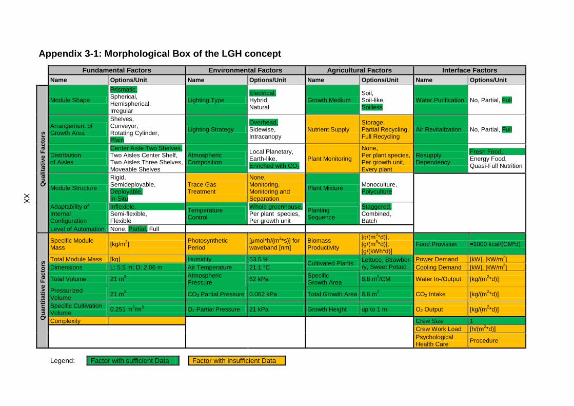
Appendix 3-1: Morphological Box of the LGH concept
Fundamental Factors Environmental Factors Agricultural Factors Interface Factors
Name Options/Unit Name Options/Unit Name Options/Unit Name Options/Unit
Qu
ali
tati
ve
Fa
cto
rs
Module Shape
Prismatic, Spherical, Hemispherical, Irregular
Lighting Type Electrical, Hybrid, Natural
Growth Medium Soil, Soil-like, Soilless
Water Purification No, Partial, Full
Arrangement of Growth Area
Shelves, Conveyor, Rotating Cylinder, Plain
Lighting Strategy Overhead, Sidewise, Intracanopy
Nutrient Supply Storage, Partial Recycling, Full Recycling
Air Revitalization No, Partial, Full
Distribution of Aisles
Center Aisle Two Shelves, Two Aisles Center Shelf, Two Aisles Three Shelves, Moveable Shelves
Atmospheric Composition
Local Planetary, Earth-like, Enriched with CO2
Plant Monitoring
None, Per plant species, Per growth unit, Every plant
Resupply Dependency
Fresh Food, Energy Food, Quasi-Full Nutrition
Module Structure
Rigid, Semideployable, Deployable, In-Situ
Trace Gas Treatment
None, Monitoring, Monitoring and Separation
Plant Mixture Monoculture, Polyculture
Adaptability of Internal Configuration
Inflexible, Semi-flexible, Flexible
Temperature Control
Whole greenhouse, Per plant species, Per growth unit
Planting Sequence
Staggered, Combined, Batch
Level of Automation None, Partial, Full
Qu
an
tita
tive
Fa
cto
rs
Specific Module Mass
[kg/m2]
Photosynthetic Period
[μmol*h/(m2*s)] for
waveband [nm] Biomass Productivity
[g/(m2*d)],
[g/(m3*d)],
[g/(kWh*d)] Food Provision ≈1000 kcal/(CM*d)
Total Module Mass [kg] Humidity 53.5 % Cultivated Plants
Lettuce, Strawber-ry, Sweet Potato
Power Demand [kW], [kW/m2]
Dimensions L: 5.5 m; D: 2.06 m Air Temperature 21.1 °C Cooling Demand [kW], [kW/m2]
Total Volume 21 m3
Atmospheric Pressure
62 kPa Specific Growth Area
8.8 m2/CM Water In-/Output [kg/(m
2*d)]
Pressurized Volume
21 m3 CO2 Partial Pressure 0.062 kPa Total Growth Area 8.8 m
2 CO2 Intake [kg/(m
2*d)]
Specific Cultivation Volume
0.251 m3/m
3 O2 Partial Pressure 21 kPa Growth Height up to 1 m O2 Output [kg/(m
2*d)]
Complexity Crew Size 1
Crew Work Load [h/(m2*d)]
Psychological Health Care
Procedure
Legend: Factor with sufficient Data Factor with insufficient Data
XX

Appendix 3-2: Morphological Box of the Lunar FARM concept
Fundamental Factors Environmental Factors Agricultural Factors Interface Factors
Name Options/Unit Name Options/Unit Name Options/Unit Name Options/Unit
Qu
ali
tati
ve
Fa
cto
rs
Module Shape
Prismatic, Spherical, Hemispherical, Irregular
Lighting Type Electrical, Hybrid, Natural
Growth Medium Soil, Soil-like, Soilless
Water Purification No, Partial, Full
Arrangement of Growth Area
Shelves, Conveyor, Rotating Cylinder, Plain
Lighting Strategy Overhead, Sidewise, Intracanopy
Nutrient Supply Storage, Partial Recycling, Full Recycling
Air Revitalization No, Partial, Full
Distribution of Aisles
Center Aisle Two Shelves, Two Aisles Center Shelf, Two Aisles Three Shelves, Moveable Shelves
Atmospheric Composition
Local Planetary, Earth-like, Enriched with CO2
Plant Monitoring
None, Per plant species, Per growth unit, Every plant
Resupply Dependency
Fresh Food, Energy Food, Quasi-Full Nutrition
Module Structure
Rigid, Semideployable, Deployable, In-Situ
Trace Gas Treatment
None, Monitoring, Monitoring and Separation
Plant Mixture Monoculture, Polyculture
Adaptability of Internal Configuration
Inflexible, Semi-flexible, Flexible
Temperature Control
Whole greenhouse, Per plant species, Per growth unit
Planting Sequence
Staggered, Combined, Batch
Level of Automation None, Partial, Full
Qu
an
tita
tive
Fa
cto
rs
Specific Module Mass
55.56 kg/m2
Photosynthetic Period
[μmol*h/(m2*s)] for
waveband [nm] Biomass Productivity
179.2 g/(m2*d) Food Provision 1753 kcal/(CM*d)
Total Module Mass 8000 kg Humidity 25 – 75 %
Cultivated Plants
Beans, Carrot, Green Onion, Pepper, White Potato, Straw-berry, Tomato, Wheat
Power Demand [kW], [kW/m2]
Dimensions L: 12.0 m; D: 8.0 m Air Temperature 17 – 28 °C Cooling Demand [kW], [kW/m2]
Total Volume 603.2 m3
Atmospheric Pressure
75.5 kPa Water In-/Output 0.252 kg/(m2*d)
Pressurized Volume
432 m3 CO2 Partial Pressure 0.02 kPa CO2 Intake [kg/(m
2*d)]
Specific Cultivation Volume
0.128 m3/m
3 O2 Partial Pressure 21.1 kPa
Specific Growth Area
27 m2/CM O2 Output 1.0 kg/(m
2*d)
Complexity Total Growth Area 144 m2 Crew Size 4.5
Growth Height 0.5 m: 96 m² 0.3 m: 48 m²
Crew Work Load 0.069 h/(m2*d)
Psychological Health Care
Procedure
Legend: Factor with sufficient Data Factor with insufficient Data
XX
I

Appendix 3-3: Morphological Box of the BIO-Plex concept
Fundamental Factors Environmental Factors Agricultural Factors Interface Factors
Name Options/Unit Name Options/Unit Name Options/Unit Name Options/Unit
Qu
ali
tati
ve
Fa
cto
rs
Module Shape
Prismatic, Spherical, Hemispherical, Irregular
Lighting Type Electrical, Hybrid, Natural
Growth Medium Soil, Soil-like, Soilless
Water Purification No, Partial, Full
Arrangement of Growth Area
Shelves, Conveyor, Rotating Cylinder, Plain
Lighting Strategy Overhead, Sidewise, Intracanopy
Nutrient Supply Storage, Partial Recycling, Full Recycling
Air Revitalization No, Partial, Full
Distribution of Aisles
Center Aisle Two Shelves, Two Aisles Center Shelf, Two Aisles Three Shelves, Moveable Shelves
Atmospheric Composition
Local Planetary, Earth-like, Enriched with CO2
Plant Monitoring
None, Per plant species, Per growth unit, Every plant
Resupply Dependency
Fresh Food, Energy Food, Quasi-Full Nutrition
Module Structure
Rigid, Semideployable, Deployable, In-Situ
Trace Gas Treatment
None, Monitoring, Monitoring and Separation
Plant Mixture Monoculture, Polyculture
Adaptability of Internal Configuration
Inflexible, Semi-flexible, Flexible
Temperature Control
Whole greenhouse, Per plant species, Per growth unit
Planting Sequence
Staggered, Combined, Batch
Level of Automation None, Partial, Full
Qu
an
tita
tive
Fa
cto
rs
Specific Module Mass
[kg/m2]
Photosynthetic Period
[μmol*h/(m2*s)] for
waveband [nm] Biomass Productivity
[g/(m2*d)],
[g/(m3*d)],
[g/(kWh*d)] Food Provision 2200 kcal/(CM*d)
Total Module Mass [kg] Humidity 65 – 85 %
Cultivated Plants
e.g.: Wheat, Rice, White Potato, Soybean, Peanut, Lettuce, Chard, …
Power Demand [kW], [kW/m2]
Dimensions L: 11.3 m; D: 4.6 m Air Temperature 16 – 35 °C Cooling Demand [kW], [kW/m2]
Total Volume 187.8 m3
Atmospheric Pressure
101 kPa Water In-/Output [kg/(m2*d)]
Pressurized Volume
187.8 m3 CO2 Partial Pressure 0.03 – 1.0 kPa Total Growth Area 82.4 m
2 CO2 Intake [kg/(m
2*d)]
Specific Cultivation Volume
0.227 m3/m
3 O2 Partial Pressure 20 – 24 kPa
Specific Growth Area
20.6 m2/CM O2 Output [kg/(m
2*d)]
Complexity
Growth Height
0.40 m: 6.6 m² 0.44 m: 6.6 m² 0.50 m: 56.8 m² 0.70 m: 12.4 m²
Crew Size 4
Crew Work Load [h/(m2*d)]
Psychological Health Care
Procedure
Legend: Factor with sufficient Data Factor with insufficient Data
XX
II
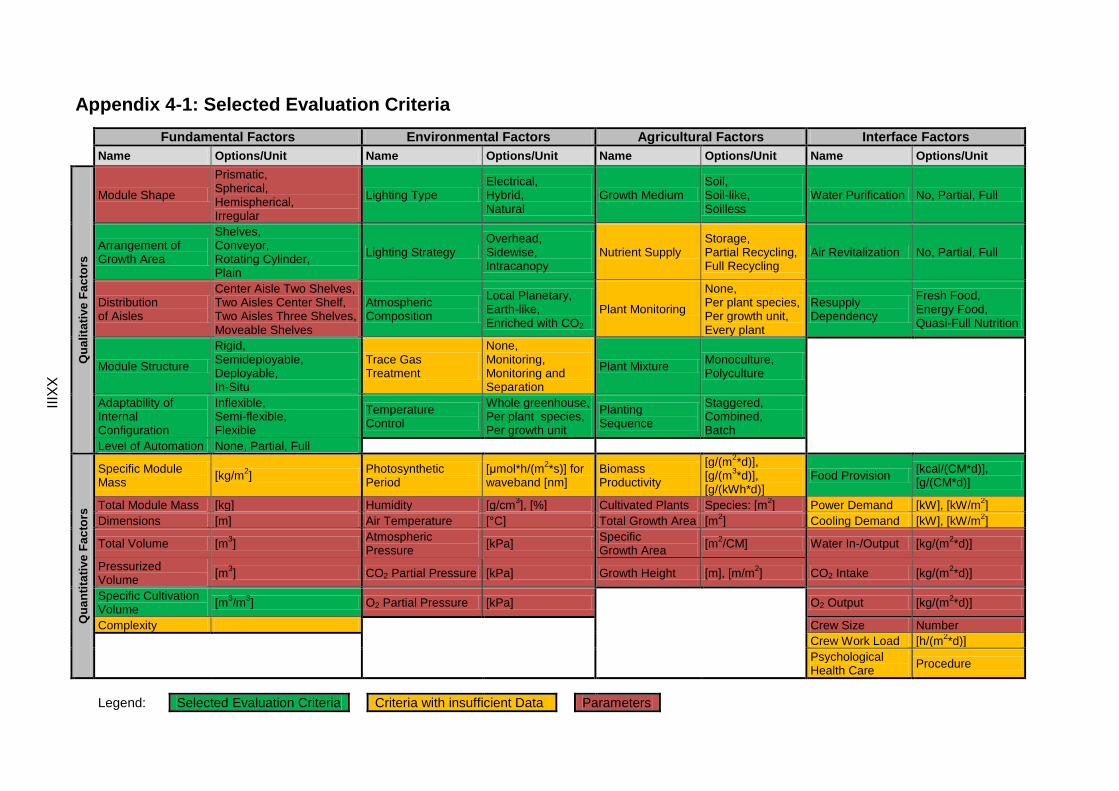
Appendix 4-1: Selected Evaluation Criteria
Fundamental Factors Environmental Factors Agricultural Factors Interface Factors
Name Options/Unit Name Options/Unit Name Options/Unit Name Options/Unit
Qu
ali
tati
ve
Fa
cto
rs
Module Shape
Prismatic, Spherical, Hemispherical, Irregular
Lighting Type Electrical, Hybrid, Natural
Growth Medium Soil, Soil-like, Soilless
Water Purification No, Partial, Full
Arrangement of Growth Area
Shelves, Conveyor, Rotating Cylinder, Plain
Lighting Strategy Overhead, Sidewise, Intracanopy
Nutrient Supply Storage, Partial Recycling, Full Recycling
Air Revitalization No, Partial, Full
Distribution of Aisles
Center Aisle Two Shelves, Two Aisles Center Shelf, Two Aisles Three Shelves, Moveable Shelves
Atmospheric Composition
Local Planetary, Earth-like, Enriched with CO2
Plant Monitoring
None, Per plant species, Per growth unit, Every plant
Resupply Dependency
Fresh Food, Energy Food, Quasi-Full Nutrition
Module Structure
Rigid, Semideployable, Deployable, In-Situ
Trace Gas Treatment
None, Monitoring, Monitoring and Separation
Plant Mixture Monoculture, Polyculture
Adaptability of Internal Configuration
Inflexible, Semi-flexible, Flexible
Temperature Control
Whole greenhouse, Per plant species, Per growth unit
Planting Sequence
Staggered, Combined, Batch
Level of Automation None, Partial, Full
Qu
an
tita
tive
Fa
cto
rs
Specific Module Mass
[kg/m2]
Photosynthetic Period
[μmol*h/(m2*s)] for
waveband [nm] Biomass Productivity
[g/(m2*d)],
[g/(m3*d)],
[g/(kWh*d)] Food Provision
[kcal/(CM*d)], [g/(CM*d)]
Total Module Mass [kg] Humidity [g/cm3], [%] Cultivated Plants Species: [m
2] Power Demand [kW], [kW/m
2]
Dimensions [m] Air Temperature [°C] Total Growth Area [m2] Cooling Demand [kW], [kW/m
2]
Total Volume [m3]
Atmospheric Pressure
[kPa] Specific Growth Area
[m2/CM] Water In-/Output [kg/(m
2*d)]
Pressurized Volume
[m3] CO2 Partial Pressure [kPa] Growth Height [m], [m/m
2] CO2 Intake [kg/(m
2*d)]
Specific Cultivation Volume
[m3/m
3] O2 Partial Pressure [kPa] O2 Output [kg/(m
2*d)]
Complexity Crew Size Number
Crew Work Load [h/(m2*d)]
Psychological Health Care
Procedure
Legend: Selected Evaluation Criteria Criteria with insufficient Data Parameters
XX
III
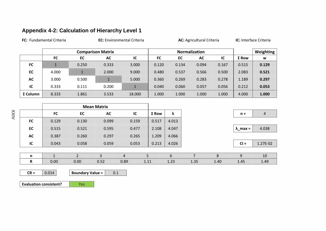
Appendix 4-2: Calculation of Hierarchy Level 1
FC: Fundamental Criteria
EC: Environmental Criteria
AC: Agricultural Criteria
IC: Interface Criteria
Comparison Matrix Normalization
Weighting FC EC AC IC FC EC AC IC Σ Row w
FC 1 0.250 0.333 3.000 0.120 0.134 0.094 0.167 0.515 0.129
EC 4.000 1 2.000 9.000 0.480 0.537 0.566 0.500 2.083 0.521
AC 3.000 0.500 1 5.000 0.360 0.269 0.283 0.278 1.189 0.297
IC 0.333 0.111 0.200 1 0.040 0.060 0.057 0.056 0.212 0.053
Σ Column 8.333 1.861 3.533 18.000 1.000 1.000 1.000 1.000 4.000 1.000
Mean Matrix
FC EC AC IC Σ Row λ
n = 4
FC 0.129 0.130 0.099 0.159 0.517 4.013
EC 0.515 0.521 0.595 0.477 2.108 4.047
λ_max = 4.038
AC 0.387 0.260 0.297 0.265 1.209 4.066
IC 0.043 0.058 0.059 0.053 0.213 4.026
CI = 1.27E-02
n 1 2 3 4 5 6 7 8 9 10 R 0.00 0.00 0.52 0.89 1.11 1.23 1.35 1.40 1.45 1.49
CR = 0.014
Boundary Value = 0.1
Evaluation consistent? Yes
XX
IV
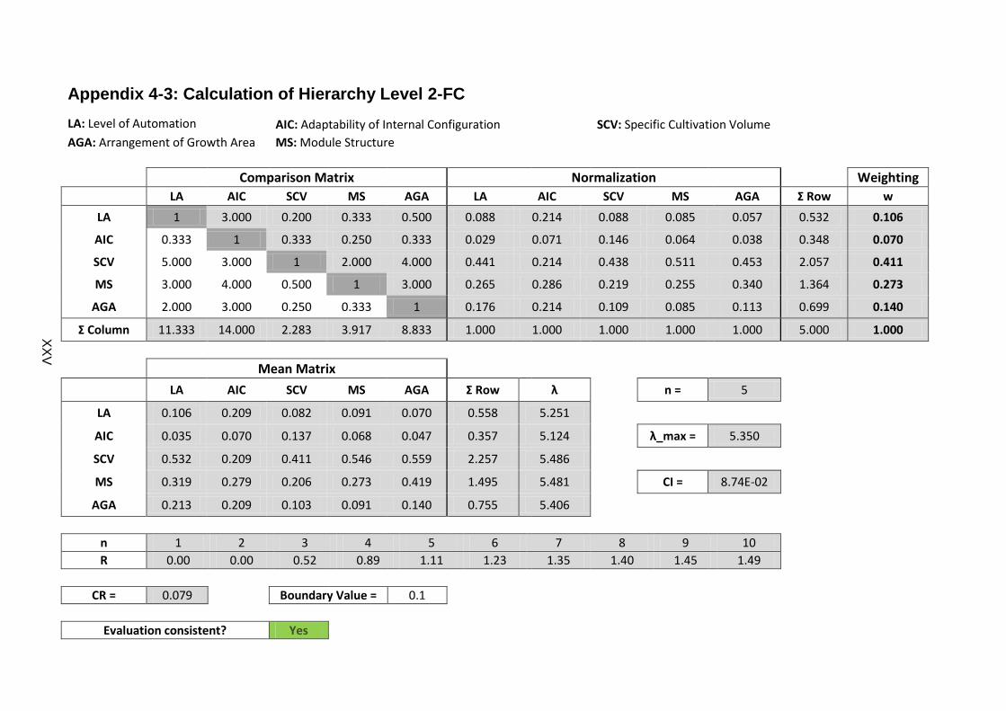
Appendix 4-3: Calculation of Hierarchy Level 2-FC
LA: Level of Automation AIC: Adaptability of Internal Configuration SCV: Specific Cultivation Volume AGA: Arrangement of Growth Area MS: Module Structure
Comparison Matrix Normalization
Weighting
LA AIC SCV MS AGA LA AIC SCV MS AGA Σ Row w
LA 1 3.000 0.200 0.333 0.500 0.088 0.214 0.088 0.085 0.057 0.532 0.106
AIC 0.333 1 0.333 0.250 0.333 0.029 0.071 0.146 0.064 0.038 0.348 0.070
SCV 5.000 3.000 1 2.000 4.000 0.441 0.214 0.438 0.511 0.453 2.057 0.411
MS 3.000 4.000 0.500 1 3.000 0.265 0.286 0.219 0.255 0.340 1.364 0.273
AGA 2.000 3.000 0.250 0.333 1 0.176 0.214 0.109 0.085 0.113 0.699 0.140
Σ Column 11.333 14.000 2.283 3.917 8.833 1.000 1.000 1.000 1.000 1.000 5.000 1.000
Mean Matrix
LA AIC SCV MS AGA Σ Row λ
n = 5
LA 0.106 0.209 0.082 0.091 0.070 0.558 5.251
AIC 0.035 0.070 0.137 0.068 0.047 0.357 5.124
λ_max = 5.350
SCV 0.532 0.209 0.411 0.546 0.559 2.257 5.486
MS 0.319 0.279 0.206 0.273 0.419 1.495 5.481
CI = 8.74E-02
AGA 0.213 0.209 0.103 0.091 0.140 0.755 5.406
n 1 2 3 4 5 6 7 8 9 10 R 0.00 0.00 0.52 0.89 1.11 1.23 1.35 1.40 1.45 1.49
CR = 0.079
Boundary Value = 0.1
Evaluation consistent? Yes
XX
V

Appendix 4-4: Calculation of Hierarchy Level 3-FC-LA
Level of Automation
Comparison Matrix Normalization
Weighting
None Partial Full None Partial Full Σ Row w
None 1 0.333 0.111 0.077 0.045 0.087 0.209 0.070
Partial 3.000 1 0.167 0.231 0.136 0.130 0.498 0.166
Full 9.000 6.000 1 0.692 0.818 0.783 2.293 0.764
Σ Column 13.000 7.333 1.278 1.000 1.000 1.000 3.000 1.000
Mean Matrix
None Partial Full Σ Row λ
n = 3
None 0.070 0.055 0.085 0.210 3.009
Partial 0.209 0.166 0.127 0.503 3.030
λ_max = 3.054
Full 0.628 0.995 0.764 2.388 3.124
CI = 2.72E-02
n 1 2 3 4 5 6 7 8 9 10 R 0.00 0.00 0.52 0.89 1.11 1.23 1.35 1.40 1.45 1.49
CR = 0.052
Boundary Value = 0.1
Evaluation consistent? Yes
XX
VI
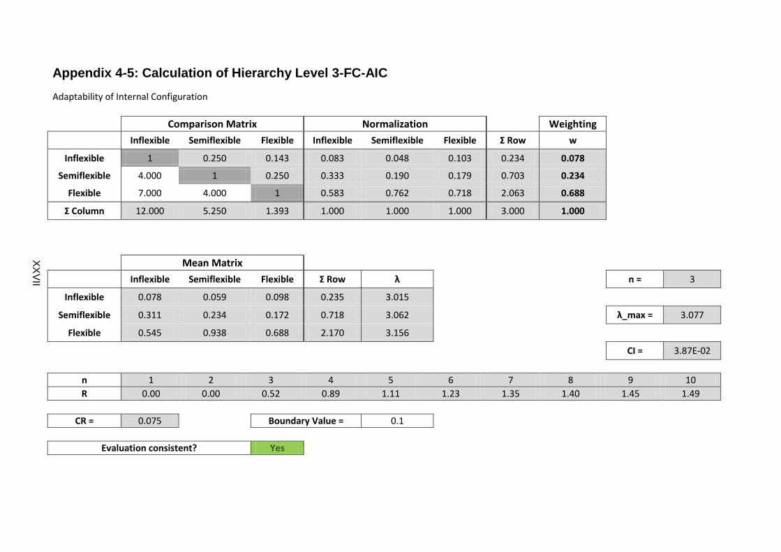
Appendix 4-5: Calculation of Hierarchy Level 3-FC-AIC
Adaptability of Internal Configuration
Comparison Matrix Normalization
Weighting
Inflexible Semiflexible Flexible Inflexible Semiflexible Flexible Σ Row w
Inflexible 1 0.250 0.143 0.083 0.048 0.103 0.234 0.078
Semiflexible 4.000 1 0.250 0.333 0.190 0.179 0.703 0.234
Flexible 7.000 4.000 1 0.583 0.762 0.718 2.063 0.688
Σ Column 12.000 5.250 1.393 1.000 1.000 1.000 3.000 1.000
Mean Matrix Inflexible Semiflexible Flexible Σ Row λ
n = 3
Inflexible 0.078 0.059 0.098 0.235 3.015
Semiflexible 0.311 0.234 0.172 0.718 3.062
λ_max = 3.077
Flexible 0.545 0.938 0.688 2.170 3.156
CI = 3.87E-02
n 1 2 3 4 5 6 7 8 9 10
R 0.00 0.00 0.52 0.89 1.11 1.23 1.35 1.40 1.45 1.49
CR = 0.075
Boundary Value = 0.1
Evaluation consistent? Yes
XX
VII
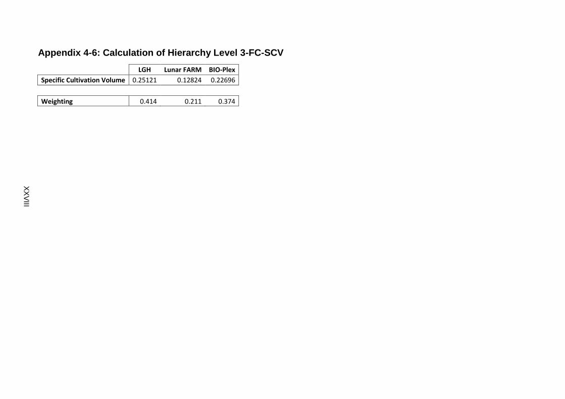
Appendix 4-6: Calculation of Hierarchy Level 3-FC-SCV
LGH Lunar FARM BIO-Plex
Specific Cultivation Volume 0.25121 0.12824 0.22696
Weighting 0.414 0.211 0.374
XX
VIII
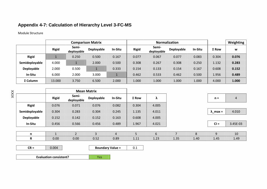
Appendix 4-7: Calculation of Hierarchy Level 3-FC-MS
Module Structure
Comparison Matrix Normalization
Weighting
Rigid
Semi-deployable
Deployable In-Situ Rigid Semi-
deployable Deployable In-Situ Σ Row w
Rigid 1 0.250 0.500 0.167 0.077 0.067 0.077 0.083 0.304 0.076
Semideployable 4.000 1 2.000 0.500 0.308 0.267 0.308 0.250 1.132 0.283
Deployable 2.000 0.500 1 0.333 0.154 0.133 0.154 0.167 0.608 0.152
In-Situ 6.000 2.000 3.000 1 0.462 0.533 0.462 0.500 1.956 0.489
Σ Column 13.000 3.750 6.500 2.000 1.000 1.000 1.000 1.000 4.000 1.000
Mean Matrix
Rigid
Semi-deployable
Deployable In-Situ Σ Row λ
n = 4
Rigid 0.076 0.071 0.076 0.082 0.304 4.005
Semideployable 0.304 0.283 0.304 0.245 1.135 4.011
λ_max = 4.010
Deployable 0.152 0.142 0.152 0.163 0.608 4.005
In-Situ 0.456 0.566 0.456 0.489 1.967 4.021
CI = 3.45E-03
n 1 2 3 4 5 6 7 8 9 10
R 0.00 0.00 0.52 0.89 1.11 1.23 1.35 1.40 1.45 1.49
CR = 0.004
Boundary Value = 0.1
Evaluation consistent? Yes
XX
IX

Appendix 4-8: Calculation of Hierarchy Level 3-FC-AGA
Arrangement of Growth Area
Comparison Matrix Normalization
Weighting
Shelves Conveyor
Rotating Cylinder
Plain Shelves Conveyor Rotating Cylinder
Plain Σ Row w
Shelves 1 3.000 5.000 9.000 0.608 0.646 0.600 0.450 2.304 0.576
Conveyor 0.333 1 2.000 7.000 0.203 0.215 0.240 0.350 1.008 0.252
Rotating Cylinder 0.200 0.500 1 3.000 0.122 0.108 0.120 0.150 0.499 0.125
Plain 0.111 0.143 0.333 1 0.068 0.031 0.040 0.050 0.188 0.047
Σ Column 1.644 4.643 8.333 20.000 1.000 1.000 1.000 1.000 4.000 1.000
Mean Matrix Shelves Conveyor
Rotating Cylinder
Plain Σ Row λ
n = 4
Shelves 0.576 0.756 0.624 0.424 2.380 4.132
Conveyor 0.192 0.252 0.250 0.330 1.023 4.060
λ_max = 4.066
Rotating Cylinder 0.115 0.126 0.125 0.141 0.507 4.064
Plain 0.064 0.036 0.042 0.047 0.189 4.008
CI = 2.20E-02
n 1 2 3 4 5 6 7 8 9 10
R 0.00 0.00 0.52 0.89 1.11 1.23 1.35 1.40 1.45 1.49
CR = 0.025
Boundary Value = 0.1
Evaluation consistent? Yes
XX
X

Appendix 4-9: Calculation of Hierarchy Level 2-EC
LT: Lighting Type LS: Lighting Strategy
AtC: Atmospheric Composition
TC: Temperature Control
Comparison Matrix Normalization
Weighting
LT LS AtC TC LT LS AtC TC Σ Row w
LT 1 3.000 2.000 5.000 0.492 0.409 0.522 0.455 1.877 0.469
LS 0.333 1 0.333 3.000 0.164 0.136 0.087 0.273 0.660 0.165
AtC 0.500 3.000 1 2.000 0.246 0.409 0.261 0.182 1.098 0.274
TC 0.200 0.333 0.500 1 0.098 0.045 0.130 0.091 0.365 0.091
Σ Column 2.033 7.333 3.833 11.000 1.000 1.000 1.000 1.000 4.000 1.000
Mean Matrix LT LS AtC TC Σ Row λ
n = 4
LT 0.469 0.495 0.549 0.456 1.970 4.197
LS 0.156 0.165 0.091 0.274 0.687 4.162
λ_max = 4.204
AtC 0.235 0.495 0.274 0.183 1.187 4.324
TC 0.094 0.055 0.137 0.091 0.377 4.134
CI = 6.81E-02
n 1 2 3 4 5 6 7 8 9 10
R 0.00 0.00 0.52 0.89 1.11 1.23 1.35 1.40 1.45 1.49
CR = 0.076
Boundary Value = 0.1
Evaluation consistent? Yes
XX
XI

Appendix 4-10: Calculation of Hierarchy Level 3-EC-LT
Lighting Type
Comparison Matrix Normalization
Weighting
Electrical Hybrid Natural Electrical Hybrid Natural Σ Row w
Electrical 1 3.000 1.000 0.429 0.429 0.429 1.286 0.429
Hybrid 0.333 1 0.333 0.143 0.143 0.143 0.429 0.143
Natural 1.000 3.000 1 0.429 0.429 0.429 1.286 0.429
Σ Column 2.333 7.000 2.333 1.000 1.000 1.000 3.000 1.000
Mean Matrix
Electrical Hybrid Natural Σ Row λ
n = 3
Electrical 0.429 0.429 0.429 1.286 3.000
Hybrid 0.143 0.143 0.143 0.429 3.000
λ_max = 3.000
Natural 0.429 0.429 0.429 1.286 3.000
CI = 0.00E+00
n 1 2 3 4 5 6 7 8 9 10
R 0.00 0.00 0.52 0.89 1.11 1.23 1.35 1.40 1.45 1.49
CR = 0.000
Boundary Value = 0.1
Evaluation consistent? Yes
XX
XII

Appendix 4-11: Calculation of Hierarchy Level 4-EC-LT-EL
HPS: High Pressure Sodium MH: Metal Halide LED: Light Emitting Diode
Comparison Matrix Normalization
Weighting
HPS MH Fluorescent Sulfur Lamps LED HPS MH Fluorescent Sulfur Lamps LED Σ Row w
HPS 1 2.000 1.000 0.333 0.125 0.074 0.100 0.074 0.069 0.074 0.391 0.078
MH 0.500 1 0.500 0.167 0.111 0.037 0.050 0.037 0.034 0.066 0.224 0.045
Fluorescent 1.000 2.000 1 0.333 0.125 0.074 0.100 0.074 0.069 0.074 0.391 0.078
Sulfur Lamps 3.000 6.000 3.000 1 0.333 0.222 0.300 0.222 0.207 0.197 1.148 0.230
LED 8.000 9.000 8.000 3.000 1 0.593 0.450 0.593 0.621 0.590 2.846 0.569
Σ Column 13.500 20.000 13.500 4.833 1.694 1.000 1.000 1.000 1.000 1.000 5.000 1.000
Mean Matrix
HPS MH Fluorescent Sulfur Lamps LED Σ Row λ
n = 5
HPS 0.078 0.090 0.078 0.077 0.071 0.394 5.036
MH 0.039 0.045 0.039 0.038 0.063 0.225 5.009
λ_max = 5.047
Fluorescent 0.078 0.090 0.078 0.077 0.071 0.394 5.036
Sulfur Lamps 0.235 0.269 0.235 0.230 0.190 1.157 5.041
CI = 1.19E-02
LED 0.625 0.403 0.625 0.689 0.569 2.912 5.116
n 1 2 3 4 5 6 7 8 9 10
R 0.00 0.00 0.52 0.89 1.11 1.23 1.35 1.40 1.45 1.49
CR = 0.011
Boundary Value = 0.1
Evaluation consistent? Yes
XX
XIII
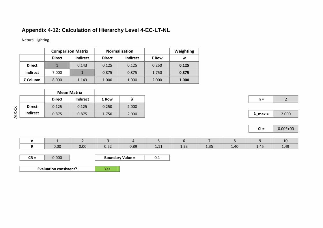
Appendix 4-12: Calculation of Hierarchy Level 4-EC-LT-NL
Natural Lighting
Comparison Matrix Normalization
Weighting
Direct Indirect Direct Indirect Σ Row w
Direct 1 0.143 0.125 0.125 0.250 0.125
Indirect 7.000 1 0.875 0.875 1.750 0.875
Σ Column 8.000 1.143 1.000 1.000 2.000 1.000
Mean Matrix
Direct Indirect Σ Row λ
n = 2
Direct 0.125 0.125 0.250 2.000
Indirect 0.875 0.875 1.750 2.000
λ_max = 2.000
CI = 0.00E+00
n 1 2 3 4 5 6 7 8 9 10
R 0.00 0.00 0.52 0.89 1.11 1.23 1.35 1.40 1.45 1.49
CR = 0.000
Boundary Value = 0.1
Evaluation consistent? Yes
XX
XIV
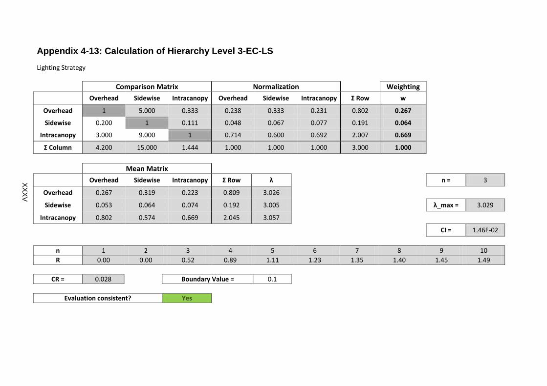
Appendix 4-13: Calculation of Hierarchy Level 3-EC-LS
Lighting Strategy
Comparison Matrix Normalization
Weighting
Overhead Sidewise Intracanopy Overhead Sidewise Intracanopy Σ Row w
Overhead 1 5.000 0.333 0.238 0.333 0.231 0.802 0.267
Sidewise 0.200 1 0.111 0.048 0.067 0.077 0.191 0.064
Intracanopy 3.000 9.000 1 0.714 0.600 0.692 2.007 0.669
Σ Column 4.200 15.000 1.444 1.000 1.000 1.000 3.000 1.000
Mean Matrix
Overhead Sidewise Intracanopy Σ Row λ
n = 3
Overhead 0.267 0.319 0.223 0.809 3.026
Sidewise 0.053 0.064 0.074 0.192 3.005
λ_max = 3.029
Intracanopy 0.802 0.574 0.669 2.045 3.057
CI = 1.46E-02
n 1 2 3 4 5 6 7 8 9 10
R 0.00 0.00 0.52 0.89 1.11 1.23 1.35 1.40 1.45 1.49
CR = 0.028
Boundary Value = 0.1
Evaluation consistent? Yes
XX
XV

Appendix 4-14: Calculation of Hierarchy Level 3-EC-AtC
Atmopsheric Composition
Comparison Matrix Normalization
Weighting
Local Plane-
tary Earth-Like
Enriched with CO2
Local Plane-tary
Earth-Like Enriched with
CO2 Σ Row w
Local Planetary 1 1.000 0.111 0.091 0.091 0.091 0.273 0.091
Earth-Like 1.000 1 0.111 0.091 0.091 0.091 0.273 0.091
Enriched with CO2
9.000 9.000 1 0.818 0.818 0.818 2.455 0.818
Σ Column 11.000 11.000 1.222 1.000 1.000 1.000 3.000 1.000
Mean Matrix Local Plane-
tary Earth-Like
Enriched with CO2
Σ Row λ
n = 3
Local Planetary 0.091 0.091 0.091 0.273 3.000
Earth-Like 0.091 0.091 0.091 0.273 3.000
λ_max = 3.000
Enriched with CO2
0.818 0.818 0.818 2.455 3.000
CI = 0.00E+00
n 1 2 3 4 5 6 7 8 9 10
R 0.00 0.00 0.52 0.89 1.11 1.23 1.35 1.40 1.45 1.49
CR = 0.000
Boundary Value = 0.1
Evaluation consistent? Yes
XX
XV
I

Appendix 4-15: Calculation of Hierarchy Level 3-EC-TC
Temperature Control
Comparison Matrix Normalization
Weighting
Whole Greenhouse
Per Plant Species
Per Growth Unit
Whole Greenhouse
Per Plant Species
Per Growth Unit
Σ Row w
Whole Greenhouse 1 0.333 0.125 0.083 0.077 0.086 0.246 0.082
Per Plant Species 3.000 1 0.333 0.250 0.231 0.229 0.709 0.236
Per Growth Unit 8.000 3.000 1 0.667 0.692 0.686 2.045 0.682
Σ Column 12.000 4.333 1.458 1.000 1.000 1.000 3.000 1.000
Mean Matrix Whole
Greenhouse Per Plant Species
Per Growth Unit
Σ Row λ
n = 3
Whole Greenhouse 0.082 0.079 0.085 0.246 3.000
Per Plant Species 0.246 0.236 0.227 0.710 3.001
λ_max = 3.002
Per Growth Unit 0.656 0.709 0.682 2.047 3.003
CI = 7.71E-04
n 1 2 3 4 5 6 7 8 9 10
R 0.00 0.00 0.52 0.89 1.11 1.23 1.35 1.40 1.45 1.49
CR = 0.001
Boundary Value = 0.1
Evaluation consistent? Yes
XX
XV
II
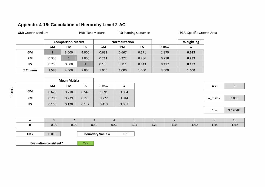
Appendix 4-16: Calculation of Hierarchy Level 2-AC
GM: Growth Medium PM: Plant Mixture PS: Planting Sequence SGA: Specific Growth Area
Comparison Matrix Normalization
Weighting GM PM PS GM PM PS Σ Row w
GM 1 3.000 4.000 0.632 0.667 0.571 1.870 0.623
PM 0.333 1 2.000 0.211 0.222 0.286 0.718 0.239
PS 0.250 0.500 1 0.158 0.111 0.143 0.412 0.137
Σ Column 1.583 4.500 7.000 1.000 1.000 1.000 3.000 1.000
Mean Matrix
GM PM PS Σ Row λ
n = 3
GM 0.623 0.718 0.549 1.891 3.034
PM 0.208 0.239 0.275 0.722 3.014
λ_max = 3.018
PS 0.156 0.120 0.137 0.413 3.007
CI = 9.17E-03
n 1 2 3 4 5 6 7 8 9 10
R 0.00 0.00 0.52 0.89 1.11 1.23 1.35 1.40 1.45 1.49
CR = 0.018
Boundary Value = 0.1
Evaluation consistent? Yes
XX
XV
III
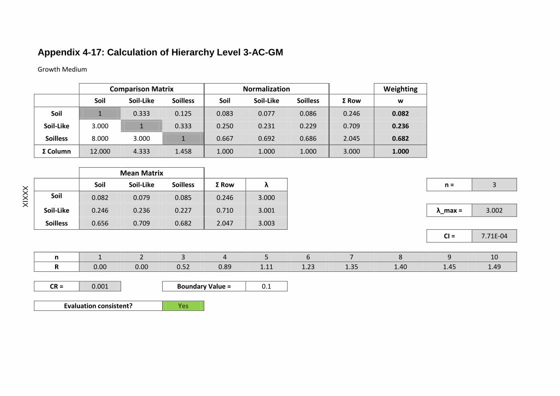
Appendix 4-17: Calculation of Hierarchy Level 3-AC-GM
Growth Medium
Comparison Matrix Normalization
Weighting
Soil Soil-Like Soilless Soil Soil-Like Soilless Σ Row w
Soil 1 0.333 0.125 0.083 0.077 0.086 0.246 0.082
Soil-Like 3.000 1 0.333 0.250 0.231 0.229 0.709 0.236
Soilless 8.000 3.000 1 0.667 0.692 0.686 2.045 0.682
Σ Column 12.000 4.333 1.458 1.000 1.000 1.000 3.000 1.000
Mean Matrix
Soil Soil-Like Soilless Σ Row λ
n = 3
Soil 0.082 0.079 0.085 0.246 3.000
Soil-Like 0.246 0.236 0.227 0.710 3.001
λ_max = 3.002
Soilless 0.656 0.709 0.682 2.047 3.003
CI = 7.71E-04
n 1 2 3 4 5 6 7 8 9 10
R 0.00 0.00 0.52 0.89 1.11 1.23 1.35 1.40 1.45 1.49
CR = 0.001
Boundary Value = 0.1
Evaluation consistent? Yes
XX
XIX

Appendix 4-18: Calculation of Hierarchy Level 4-AC-GM-S
Soil
Comparison Matrix Normalization
Weighting
Terrestrial
Extraterres-trial
Terrestrial Extraterres-
trial Σ Row w
Terrestrial 1 0.250 0.200 0.200 0.400 0.200
Extraterrestrial 4.000 1 0.800 0.800 1.600 0.800
Σ Column 5.000 1.250 1.000 1.000 2.000 1.000
Mean Matrix
Terrestrial
Extraterres-trial
Σ Row λ
n = 2
Terrestrial 0.200 0.200 0.400 2.000
Extraterrestrial 0.800 0.800 1.600 2.000
λ_max = 2.000
CI = 0.00E+00
n 1 2 3 4 5 6 7 8 9 10
R 0.00 0.00 0.52 0.89 1.11 1.23 1.35 1.40 1.45 1.49
CR = 0.000
Boundary Value = 0.1
Evaluation consistent? Yes
XL

Appendix 4-19: Calculation of Hierarchy Level 4-AC-GM-SL
Soil-Like
Comparison Matrix Normalization
Weighting
Organic Inert Organic Inert Σ Row w
Organic 1 0.200 0.167 0.167 0.333 0.167
Inert 5.000 1 0.833 0.833 1.667 0.833
Σ Column 6.000 1.200 1.000 1.000 2.000 1.000
Mean Matrix
Organic Inert Σ Row λ
n = 2
Organic 0.167 0.167 0.333 2.000
Inert 0.833 0.833 1.667 2.000
λ_max = 2.000
CI = 0.00E+00
n 1 2 3 4 5 6 7 8 9 10
R 0.00 0.00 0.52 0.89 1.11 1.23 1.35 1.40 1.45 1.49
CR = 0.000
Boundary Value = 0.1
Evaluation consistent? Yes
XL
I
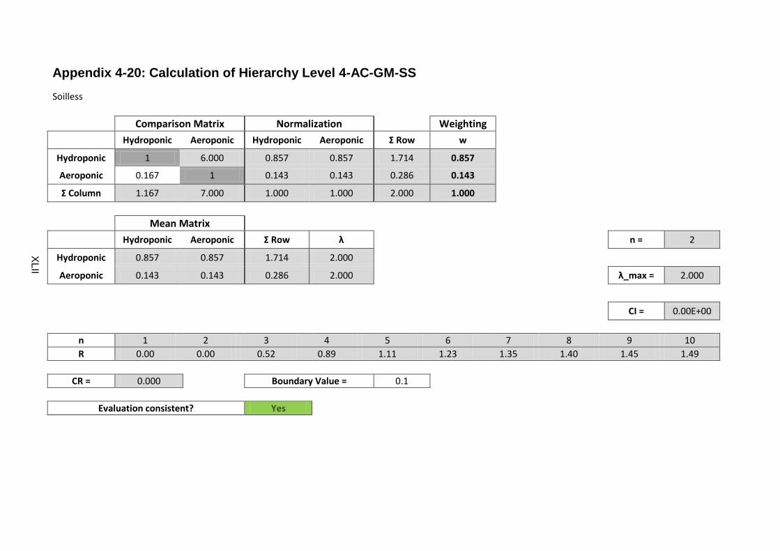
Appendix 4-20: Calculation of Hierarchy Level 4-AC-GM-SS
Soilless
Comparison Matrix Normalization
Weighting
Hydroponic Aeroponic Hydroponic Aeroponic Σ Row w
Hydroponic 1 6.000 0.857 0.857 1.714 0.857
Aeroponic 0.167 1 0.143 0.143 0.286 0.143
Σ Column 1.167 7.000 1.000 1.000 2.000 1.000
Mean Matrix
Hydroponic Aeroponic Σ Row λ
n = 2
Hydroponic 0.857 0.857 1.714 2.000
Aeroponic 0.143 0.143 0.286 2.000
λ_max = 2.000
CI = 0.00E+00
n 1 2 3 4 5 6 7 8 9 10
R 0.00 0.00 0.52 0.89 1.11 1.23 1.35 1.40 1.45 1.49
CR = 0.000
Boundary Value = 0.1
Evaluation consistent? Yes
XL
II
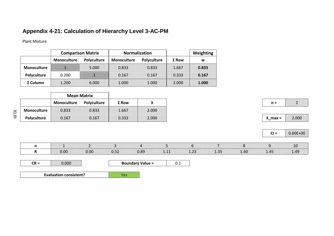
Appendix 4-21: Calculation of Hierarchy Level 3-AC-PM
Plant Mixture
Comparison Matrix Normalization
Weighting
Monoculture Polyculture Monoculture Polyculture Σ Row w
Monoculture 1 5.000 0.833 0.833 1.667 0.833
Polyculture 0.200 1 0.167 0.167 0.333 0.167
Σ Column 1.200 6.000 1.000 1.000 2.000 1.000
Mean Matrix
Monoculture Polyculture Σ Row λ
n = 2
Monoculture 0.833 0.833 1.667 2.000
Polyculture 0.167 0.167 0.333 2.000
λ_max = 2.000
CI = 0.00E+00
n 1 2 3 4 5 6 7 8 9 10
R 0.00 0.00 0.52 0.89 1.11 1.23 1.35 1.40 1.45 1.49
CR = 0.000
Boundary Value = 0.1
Evaluation consistent? Yes
XL
III

Appendix 4-22: Calculation of Hierarchy Level 3-AC-PS
Planting Sequence
Comparison Matrix Normalization
Weighting
Staggered Combined Batch Staggered Combined Batch Σ Row w
Staggered 1 0.200 1.000 0.143 0.143 0.143 0.429 0.143
Combined 5.000 1 5.000 0.714 0.714 0.714 2.143 0.714
Batch 1.000 0.200 1 0.143 0.143 0.143 0.429 0.143
Σ Column 7.000 1.400 7.000 1.000 1.000 1.000 3.000 1.000
Mean Matrix
Staggered Combined Batch Σ Row λ
n = 3
Staggered 0.143 0.143 0.143 0.429 3.000
Combined 0.714 0.714 0.714 2.143 3.000
λ_max = 3.000
Batch 0.143 0.143 0.143 0.429 3.000
CI = 0.00E+00
n 1 2 3 4 5 6 7 8 9 10
R 0.00 0.00 0.52 0.89 1.11 1.23 1.35 1.40 1.45 1.49
CR = 0.000
Boundary Value = 0.1
Evaluation consistent? Yes
XL
IV
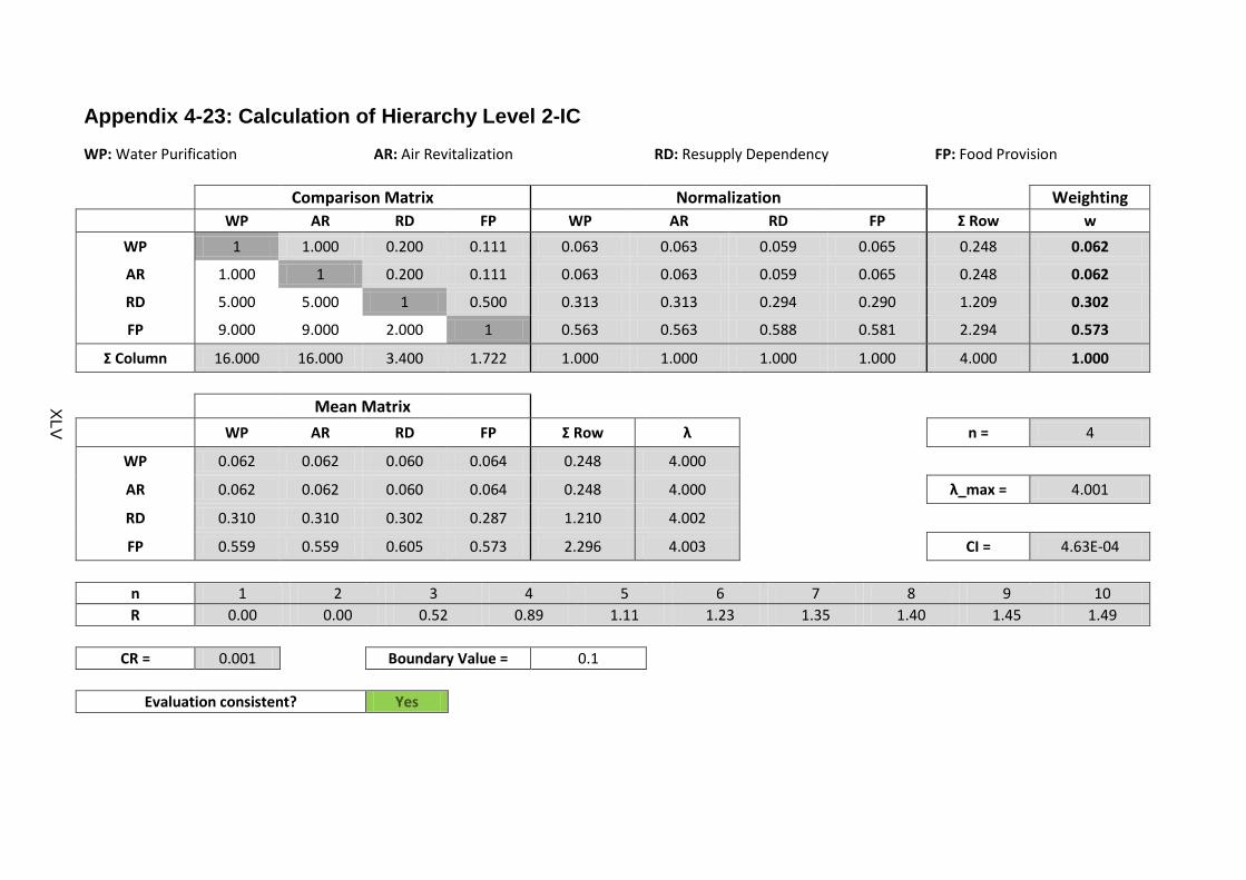
Appendix 4-23: Calculation of Hierarchy Level 2-IC
WP: Water Purification AR: Air Revitalization RD: Resupply Dependency FP: Food Provision
Comparison Matrix Normalization
Weighting
WP AR RD FP WP AR RD FP Σ Row w
WP 1 1.000 0.200 0.111 0.063 0.063 0.059 0.065 0.248 0.062
AR 1.000 1 0.200 0.111 0.063 0.063 0.059 0.065 0.248 0.062
RD 5.000 5.000 1 0.500 0.313 0.313 0.294 0.290 1.209 0.302
FP 9.000 9.000 2.000 1 0.563 0.563 0.588 0.581 2.294 0.573
Σ Column 16.000 16.000 3.400 1.722 1.000 1.000 1.000 1.000 4.000 1.000
Mean Matrix
WP AR RD FP Σ Row λ
n = 4
WP 0.062 0.062 0.060 0.064 0.248 4.000
AR 0.062 0.062 0.060 0.064 0.248 4.000
λ_max = 4.001
RD 0.310 0.310 0.302 0.287 1.210 4.002
FP 0.559 0.559 0.605 0.573 2.296 4.003
CI = 4.63E-04
n 1 2 3 4 5 6 7 8 9 10
R 0.00 0.00 0.52 0.89 1.11 1.23 1.35 1.40 1.45 1.49
CR = 0.001
Boundary Value = 0.1
Evaluation consistent? Yes
XL
V

Appendix 4-24: Calculation of Hierarchy Level 3-IC-WP
Water Purification
Comparison Matrix Normalization
Weighting
No Partial Full No Partial Full Σ Row w
No 1 0.250 0.111 0.071 0.077 0.069 0.217 0.072
Partial 4.000 1 0.500 0.286 0.308 0.310 0.904 0.301
Full 9.000 2.000 1 0.643 0.615 0.621 1.879 0.626
Σ Column 14.000 3.250 1.611 1.000 1.000 1.000 3.000 1.000
Mean Matrix
No Partial Full Σ Row λ
n = 3
No 0.072 0.075 0.070 0.217 3.000
Partial 0.290 0.301 0.313 0.904 3.001
λ_max = 3.002
Full 0.652 0.603 0.626 1.881 3.003
CI = 7.71E-04
n 1 2 3 4 5 6 7 8 9 10
R 0.00 0.00 0.52 0.89 1.11 1.23 1.35 1.40 1.45 1.49
CR = 0.001
Boundary Value = 0.1
Evaluation consistent? Yes
XL
VI

Appendix 4-25: Calculation of Hierarchy Level 3-IC-AR
Air Revitalization
Comparison Matrix Normalization
Weighting
No Partial Full No Partial Full Σ Row w
No 1 0.250 0.111 0.071 0.077 0.069 0.217 0.072
Partial 4.000 1 0.500 0.286 0.308 0.310 0.904 0.301
Full 9.000 2.000 1 0.643 0.615 0.621 1.879 0.626
Σ Column 14.000 3.250 1.611 1.000 1.000 1.000 3.000 1.000
Mean Matrix
No Partial Full Σ Row λ
n = 3
No 0.072 0.075 0.070 0.217 3.000
Partial 0.290 0.301 0.313 0.904 3.001
λ_max = 3.002
Full 0.652 0.603 0.626 1.881 3.003
CI = 7.71E-04
n 1 2 3 4 5 6 7 8 9 10
R 0.00 0.00 0.52 0.89 1.11 1.23 1.35 1.40 1.45 1.49
CR = 0.001
Boundary Value = 0.1
Evaluation consistent? Yes
XL
VII
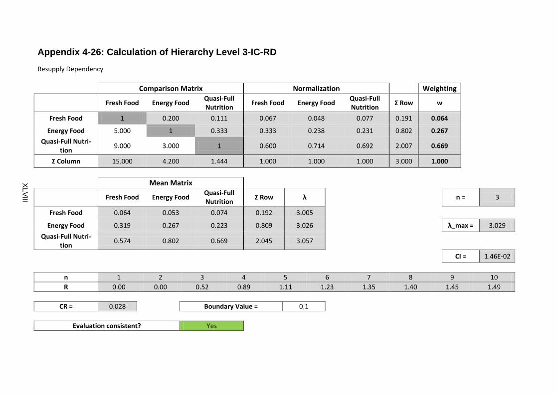
Appendix 4-26: Calculation of Hierarchy Level 3-IC-RD
Resupply Dependency
Comparison Matrix Normalization
Weighting
Fresh Food Energy Food
Quasi-Full Nutrition
Fresh Food Energy Food Quasi-Full Nutrition
Σ Row w
Fresh Food 1 0.200 0.111 0.067 0.048 0.077 0.191 0.064
Energy Food 5.000 1 0.333 0.333 0.238 0.231 0.802 0.267
Quasi-Full Nutri-tion
9.000 3.000 1 0.600 0.714 0.692 2.007 0.669
Σ Column 15.000 4.200 1.444 1.000 1.000 1.000 3.000 1.000
Mean Matrix
Fresh Food Energy Food
Quasi-Full Nutrition
Σ Row λ
n = 3
Fresh Food 0.064 0.053 0.074 0.192 3.005
Energy Food 0.319 0.267 0.223 0.809 3.026
λ_max = 3.029
Quasi-Full Nutri-tion
0.574 0.802 0.669 2.045 3.057
CI = 1.46E-02
n 1 2 3 4 5 6 7 8 9 10
R 0.00 0.00 0.52 0.89 1.11 1.23 1.35 1.40 1.45 1.49
CR = 0.028
Boundary Value = 0.1
Evaluation consistent? Yes
XL
VIII

Appendix 4-27: Calculation of Hierarchy Level 3-IC-FP
Food Provision
LGH Lunar FARM BIO-Plex
Food Provision [kcal/(CM*d)] 1000 1753 2200
Optimum = 2300 kcal/(CM*d)
Difference to Optimum 1300 547 100
Weighting 0.061062737 0.145121679 0.793815584
XL
IX
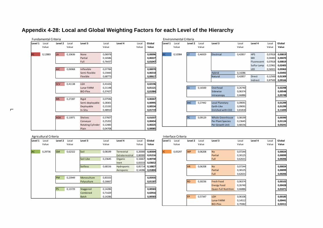
Appendix 4-28: Local and Global Weighting Factors for each Level of the Hierarchy
Level 1 Level 2 Level 3 Level 4 Level 1 Level 2 Level 3 Level 4
FC 0,12883 LA 0,10636 None 0,06978 0,00096 EC 0,52084 LT 0,46929 Electrical 0,42857 HPS 0,07818 0,00819
Partial 0,16586 0,00227 MH 0,04483 0,00470
Full 0,76437 0,01047 Fluorescent 0,07818 0,00819
Sulfur Lamp 0,22961 0,02405
AIC 0,06968 Inflexible 0,07784 0,00070 LED 0,56921 0,05963
Semi-flexible 0,23443 0,00210 Hybrid 0,14286 0,03492
Flexible 0,68773 0,00617 Natural 0,42857 Direct 0,12500 0,01309
Indirect 0,87500 0,09166
SCV 0,41138 LGH 0,41426 0,02196
Lunar FARM 0,21148 0,01121 LS 0,16500 Overhead 0,26740 0,02298
BIO-Plex 0,37427 0,01984 Sidewise 0,06374 0,00548
Intracanopy 0,66886 0,05748
MS 0,27287 Rigid 0,07596 0,00267
Semi-deployable 0,28301 0,00995 AtC 0,27442 Local Planetary 0,09091 0,01299
Deployable 0,15192 0,00534 Earth-Like 0,09091 0,01299
In-Situ 0,48910 0,01719 Enriched with CO2 0,81818 0,11694
AGA 0,13971 Shelves 0,57607 0,01037 TC 0,09129 Whole Greenhouse 0,08199 0,00390
Conveyor 0,25202 0,00454 Per Plant Species 0,23645 0,01124
Rotating Cylinder 0,12483 0,00225 Per Growth Unit 0,68156 0,03241
Plain 0,04708 0,00085
Level 1 Level 2 Level 3 Level 4 Level 1 Level 2 Level 3 Level 4
AC 0,29736 GM 0,62322 Soil 0,08199 Terrestrial 0,20000 0,00304 IC 0,05297 WP 0,06208 No 0,07244 0,00024
Extraterrestrial 0,80000 0,01216 Partial 0,30125 0,00099
Soil-Like 0,23645 Organic 0,16667 0,00730 Full 0,62631 0,00206
Inert 0,83333 0,03652
Soilless 0,68156 Hydroponic 0,85714 0,10827 AR 0,06208 No 0,07244 0,00024
Aeroponic 0,14286 0,01804 Partial 0,30125 0,00099
Full 0,62631 0,00206
PM 0,23949 Monoculture 0,83333 0,05935
Polyculture 0,16667 0,01187 RD 0,30236 Fresh Food 0,06374 0,00102
Energy Food 0,26740 0,00428
PS 0,13729 Staggered 0,14286 0,00583 Quasi-Full Nutrition 0,66886 0,01071
Combined 0,71429 0,02916
Batch 0,14286 0,00583 FP 0,57347 LGH 0,06106 0,00185
Lunar FARM 0,14512 0,00441
BIO-Plex 0,79382 0,02411
Local
Value
Local
Value
Local
Value
Global
Value
Local
Value
Local
Value
Local
Value
Local
Value
Global
Value
Local
Value
Local
Value
Local
Value
Local
Value
Global
Value
Global
Value
Local
Value
Local
Value
Local
Value
Fundamental Criteria Environmental Criteria
Agricultural Criteria Interface Criteria
Local
Value
Local
Value
L
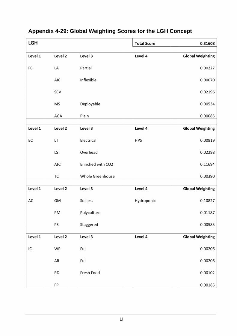
LI
Appendix 4-29: Global Weighting Scores for the LGH Concept
LGH Total Score 0.31608
Level 1 Level 2 Level 3 Level 4 Global Weighting
FC
LA
Partial
0.00227
AIC
Inflexible
0.00070
SCV
0.02196
MS
Deployable
0.00534
AGA Plain 0.00085
Level 1 Level 2 Level 3 Level 4 Global Weighting
EC
LT
Electrical
HPS
0.00819
LS
Overhead
0.02298
AtC
Enriched with CO2
0.11694
TC Whole Greenhouse 0.00390
Level 1 Level 2 Level 3 Level 4 Global Weighting
AC
GM
Soilless
Hydroponic
0.10827
PM
Polyculture
0.01187
PS
Staggered
0.00583
Level 1 Level 2 Level 3 Level 4 Global Weighting
IC
WP
Full
0.00206
AR
Full
0.00206
RD
Fresh Food
0.00102
FP 0.00185

LII
Appendix 4-30: Global Weighting Scores for the Lunar FARM Concept
Lunar FARM Total Score 0.51336
Level 1 Level 2 Level 3 Level 4 Global Weighting
FC
LA
Partial
0.00227
AIC
Semi-flexible
0.00210
SCV
0.01121
MS
Rigid
0.00267
AGA Shelves 0.01037
Level 1 Level 2 Level 3 Level 4 Global Weighting
EC
LT
Natural
Indirect
0.09166
LS
Intracanopy
0.05748
AtC
Enriched with CO2
0.11694
TC Per Growth Unit 0.03241
Level 1 Level 2 Level 3 Level 4 Global Weighting
AC
GM
Soilless
Hydroponic
0.10827
PM
Monoculture
0.05935
PS Batch 0.00583
Level 1 Level 2 Level 3 Level 4 Global Weighting
IC
WP
Full
0.00206
AR
Full
0.00206
RD
Energy Food
0.00428
FP 0.00441

LIII
Appendix 4-31: Global Weighting Scores for the BIO-Plex Concept
BIO-Plex Total Score 0.45348
Level 1 Level 2 Level 3 Level 4 Global Weighting
FC
LA
Partial
0.00227
AIC
Semi-flexible
0.00210
SCV
0.01984
MS
Rigid
0.00267
AGA Shelves 0.01037
Level 1 Level 2 Level 3 Level 4 Global Weighting
EC
LT
Electrical
HPS
0.00819
LS
Overhead
0.02298
AtC
Enriched with CO2
0.11694
TC Per Growth Unit 0.03241
Level 1 Level 2 Level 3 Level 4 Global Weighting
AC
GM
Soilless
Hydroponic
0.10827
PM
Monoculture
0.05935
PS Combined 0.02916
Level 1 Level 2 Level 3 Level 4 Global Weighting
IC
WP
Full
0.00206
AR
Full
0.00206
RD
Quasi-Full Nutrition
0.01071
FP 0.02411
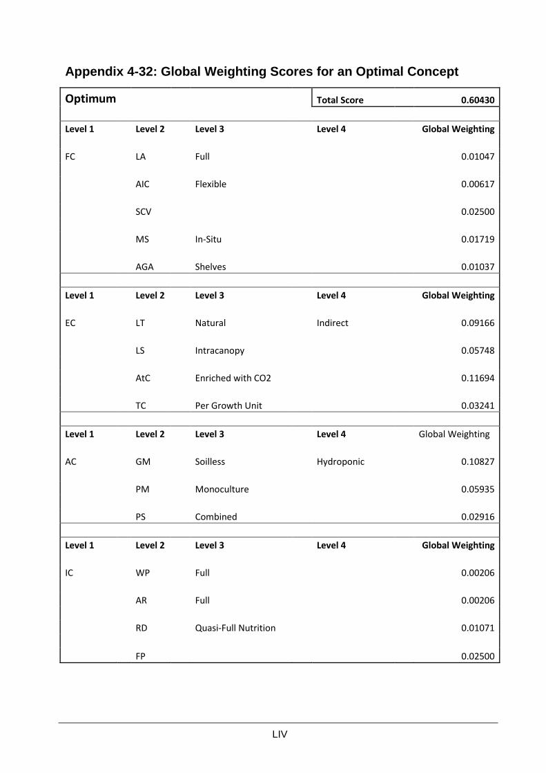
LIV
Appendix 4-32: Global Weighting Scores for an Optimal Concept
Optimum Total Score 0.60430
Level 1 Level 2 Level 3 Level 4 Global Weighting
FC
LA
Full
0.01047
AIC
Flexible
0.00617
SCV
0.02500
MS
In-Situ
0.01719
AGA Shelves 0.01037
Level 1 Level 2 Level 3 Level 4 Global Weighting
EC
LT
Natural
Indirect
0.09166
LS
Intracanopy
0.05748
AtC
Enriched with CO2
0.11694
TC Per Growth Unit 0.03241
Level 1 Level 2 Level 3 Level 4 Global Weighting
AC
GM
Soilless
Hydroponic
0.10827
PM
Monoculture
0.05935
PS Combined 0.02916
Level 1 Level 2 Level 3 Level 4 Global Weighting
IC
WP
Full
0.00206
AR
Full
0.00206
RD
Quasi-Full Nutrition
0.01071
FP 0.02500


