DISSERTATION
Price formation in electricity forward markets: An empirical analysis of
expectations and risk aversion
ausgeführt zum Zwecke der Erlangung des akademischen Grades
eines Doktors der technischen Wissenschaften
unter der Leitung von
Univ.-Prof. Dipl.-Ing. Dr.techn. Reinhard Haas
und
Prof. Dr. Derek W. Bunn
eingereicht an der Technischen Universität Wien
Fakultät für Elektrotechnik und Informationstechnik
von
Dipl.-Ing. Christian Redl
Mat.Nr. 9825692
Josefstädterstr. 82/58
1080 Wien
Wien, im März 2011 ______________________

To my family

Acknowledgements
Sincere thanks go to my supervisors Prof. Reinhard Haas and Prof. Derek Bunn. The
openness of Reinhard Haas and his comments enabled me to develop and perform research on
this topic. While I was visiting Derek Bunn’s research group at the London Business School
my research made substantial progress. I owe the crucial ideas in this thesis to the inspiring
atmosphere at his group and especially to the discussions with Derek Bunn and his comments.
Prof. Bernhard Böhm and Claus Huber took time during the past years to continuously
discuss my work in progress. Before each meeting I was not only looking forward to their
comments but also to having a nice time with them. Discussions with Benoît Sévi clarified
initially intuitive ideas.
At the Night & Day Café, Manchester, UK, the band Delphic was recording a new song while
I came up with the final outline of this thesis. This acoustic environment supported me
substantially.
At the Energy Economics Group my colleagues created an atmosphere that rendered the years
of my PhD studies particularly good. Thanks also to them.

i
Abstract
Futures and forward contracts are important means of risk reduction and transfer for market
participants in liberalised electricity markets. This is reflected in high trading volumes –
eventually exceeding actual physical demand. Sources of uncertainty and risks in power
markets are manifold and range from short, medium and long term fundamental market
uncertainties to open regulatory and policy decisions.
The theoretical literature on electricity futures markets has focused on the expectation
formation of market actors. It demonstrates how forward prices arise from expected future
spot prices. Further the literature maps the effect of risk aversion on the market outcome.
Forward premia, so it reveals, emerge from the stochastic properties of spot prices.
The objective of this thesis is to integrate concepts of expectation formation and risk
assessment of wholesale power market participants. By means of econometric models applied
to the two major European electricity markets, the thesis analyses the determinants of futures
prices and corresponding interactions between spots and forwards. The implications of these
interactions for forward premia and its components are studied.
Firstly, the models reveal a combination of fundamental and behavioural pricing components
of electricity forward prices. More precisely, the forwards are driven by estimates of future
generation costs as well as current spot and forward prices of other maturities. Secondly, this
complex price formation affects and interferes with the risk assessment of market participants
and, in turn, influences their willingness to pay for risk reduction. Forward premia, the models
show thirdly, are a compound function of fundamental, behavioural, market structure,
dynamic and external shock components. Specifically, forward premia being affected by the
unfavourable market structure in terms of concentration and market power effects unfolds
market monitoring issues.
The results, so the conclusion, question the consistency of electricity futures price quotations.
Moreover, there is an interaction effect with realised forward premia which contain
behavioural pricing components. These insights cannot rule out inefficiencies in the analysed
futures markets. In turn, futures prices and corresponding forward premia should be
considered key elements when assessing transaction costs associated with electricity
wholesale market restructuring.

ii
Kurzfassung
Terminkontrakte stellen ein wichtiges Mittel zum Risikomanagement von Akteuren in
liberalisierten Strommärkten dar. Dies widerspiegelt sich in Handelsvolumina, die die
tatsächliche Nachfrage übersteigen. Die Bandbreite von Unsicherheit und Risiken in
Strommärkten reicht von kurz-, mittel- und langfristigen Marktunsicherheiten bis offenen
regulatorischen und politischen Entscheidungen.
Die theoretische Literatur zu Stromterminmärkten fokussiert auf die Erwartungsbildung und
auf Konsequenzen von Risikoaversion. Terminpreise werden über Erwartungen künftiger
Spotpreise und Forwardprämien über die stochastischen Eigenschaften der Spotpreise erklärt.
Das Ziel dieser Arbeit ist Konzepte der Erwartungsbildung und der Risikoeinschätzung zu
integrieren. Konkret werden ökonometrische Modelle auf die zwei wichtigsten europäischen
Strommärkte angewandt um Einflussparameter von Terminpreisen sowie Wechselwirkungen
zwischen kurz- und langfristigen Preisen untersuchen zu können. Des Weiteren werden
entsprechende Implikationen für die Forwardprämien dargestellt und erklärt.
Die Modelle zeigen eine Kombination von fundamentalen und verhaltensbezogenen
Einflüssen auf die Terminpreise. Der Terminmarktpreis wird sowohl von Erwartungen
bezüglich künftiger Erzeugungskosten als auch von aktuellen Spot- und Terminpreisen
anderer Fristigkeiten beeinflusst. Diese komplexe Preisbildung beeinflusst und vermischt sich
mit der Risikobeurteilung der Marktteilnehmer und affektiert deren Zahlungsbereitschaft zur
Reduktion entsprechender Risiken. Die Modelle zeigen, dass Forwardprämien eine Funktion
von fundamentalen, verhaltensökonomischen, strukturellen und dynamischen Komponenten
sind. Weiters beeinflussen externe Schocks die Forwardprämie. Effekte von
Marktkonzentration und Marktmacht werfen Fragen zum Marktmonitoring auf.
Zusammenfassend hinterfragen die Ergebnisse die Konsistenz von Terminpreisnotierungen.
Ineffizienzen können daher in den untersuchten Terminmärkten nicht ausgeschlossen werden.
Terminpreise und korrespondierende Forwardprämien sollten als wesentliche Elemente von
Transaktionskosten interpretiert werden, die es bei der Beurteilung von liberalisierten
Strommärkten zu berücksichtigen gilt.
iii
Executive summary
Motivation
Breaking up the regulated monopoly of electricity supply in the European Union (EU) in 1997
into the potentially competitive segments of generation and supply and the regulated natural
monopoly businesses of transmission and distribution has led to an unprecedented
transformation of the industrial organisation of the power sector. Final customers and
suppliers can, since liberalisation, freely source their electricity, generators may and actually
do enter new business fields, electricity has become a tradable commodity and, accordingly,
organised market places have emerged. Thus, the usage and utilisation of the interregional
power network has changed. Not only contributes it to one of its original functions – security
of supply – but also has to abide by the laws of economics – arbitrage and profit maximisation
– nevertheless still bounded by the constraining forces of physics: Kirchhoff’s laws.
No pain no gain. Generators have to make decentralised investment decisions in an
environment of various short and long term (market and regulatory) uncertainties, consumers
are exposed to a supply side prone to the exercise of market power due to the physical
features of the commodity electricity (and its generation technologies), supply and demand
side characteristics yield a highly volatile market result, and, above all, the EU power market
has to deliver policy targets related to competitiveness, supply security and climate change.
Hence, as with any market, the sources of risk – and demands for compensation – are
manifold.
Theories of industrial organisation, regulation and financial markets have proposed various
treatments of these risks. This thesis is concerned with one potential cure: The forward
market, which should contribute to market completeness – a necessary condition for the
optimality of competitive markets – and the facilitation of risk management and risk transfer.
Specifically, it focused on the empirical assessment of major European long-term futures and
forward markets. The attractiveness of long-term markets from a risk management point of
view is reflected in high trading volumes on these markets – eventually exceeding physical
demand.
High trading volumes and, correspondingly, high market liquidity are generally considered as
indications of mature and well-functioning markets. Yet it is crucial to gain deeper insight
iv
into the price formation process – not at least because of the special characteristics of the
physical commodity electricity, associated consequences for the market structure, and its
importance for the overall economy. These insights enable an efficient and effective design of
the markets and its regulatory and legislative provisions.
Research questions
In particular, the following questions are addressed in this thesis:
1. How are expectations formed in long-term markets?
2. What are the drivers of futures and forward prices?
3. What is the effect of trading of risk averse market actors on the futures-spot bias?
4. How do market structure and supply and demand shocks affect risk assessment and
market outcomes?
5. What, in turn, are the determinants of the forward premium?
6. What are the implications for market efficiency?
Methodology
Some of the above questions are assessed by a review of the theoretical literature and by a
simple analytical equilibrium modelling approach. Most of this thesis is, however, concerned
with empirical analyses of the two main European power markets: The Central-Western
European and the Scandinavian power market. Both reduced-form regression and vector
autoregression models are applied throughout this thesis.
Theory
Forward markets deliver two main functions in an economy: They provide and aggregate
information about future prices and allow for hedging price risks (Newbery and Stiglitz,
1981). Electricity forward prices arise from an equilibrium in expectations and risk aversion
(Keynes, 1930) amongst agents with heterogeneous needs for hedging spot price uncertainty.
The forward price Ft,T quoted at time t for delivery at time T is thereby viewed as being
determined as the expected spot price E(ST) plus an ex ante forward premium FPt,T. In

v
essence, the forward premium constitutes the costs of the hedge in order to insure a fixed
price ahead of the delivery (i.e. the futures price).
Price formation in electricity forward markets: The case of year-ahead futures prices
The analysis shows that year-ahead baseload electricity prices do depend on year-ahead
generation costs in line with economic theory on equilibrium relationships for forward
pricing. The year-ahead generation costs can be interpreted as the market’s best estimate of
future electricity prices. Second, electricity forward prices are also influenced by current spot
prices. Moreover, the recent trend of spot prices has a significant impact on the futures price.
This suggests the existence of a behavioural pricing component in the forward market.
Trading strategies of market participants seem to rely partly on current spot prices instead of
fundamental modelling approaches. Finally, although the EEX and Nord Pool market are
physically only weakly interconnected – resulting in different price levels – main
characteristics with regard to price formation on the year-ahead forward markets are alike
although the supply and demand side characteristics in the EEX market differ significantly
from the fundamentals in the Nord Pool market.
Clearly, the significant influence of current spot market prices on futures prices in both
markets questions the forecasting power of the forward price (i.e. the consistency of the
forward price). Hence, it is important to study the relationship between current spot and
forward prices in detail.
Interaction between spot and forward prices
Clearing on spot and futures markets is a result of market forces and their interactions which
might suggest a simultaneous evolution. Clearly, a link between current spot and current
forward prices should not be anticipated due to the fact that electricity is not storable. Finding
a corresponding relationship, however, would reveal a strong behavioural pricing component
prevailing in the markets.
Benth et al. (2009) contend that the lacking storability of electricity implies that spot prices
are not affected by available information about future price changes (i.e. price changes in the
forward contract market). However, the results of this thesis suggest the opposite. In fact, the
vi
prevalence of behavioural components in the electricity markets’ price formation is
discernible since different product types (i.e. spots and various forwards) mutually influence
each other.
Specifically, Granger-non causality tests have revealed significant interactions among spot
price returns and month-, quarter-, and year-ahead futures price returns casting doubt on a
clear distinction between short and long term markets. This suggests the existence of
behavioural pricing components and rejects claims on a supposedly exogeneity – caused by
the non-storability of electricity – of spot prices on the one hand and forward prices on the
other. Furthermore, these results are confirmed by VAR regression models. More specifically,
the movement of the electricity price system can, to a large extent, be explained by exogenous
supply and demand side variables driving the electricity prices. Still, there are strong
interactions between the electricity price series confirmed by significant regression
coefficients in the VAR models (which accords with Granger non-causality tests). The results
of the regression models cast doubts on the predictive power of forward prices and, in turn, on
market efficiency. Besides these behavioural pricing components risk aversion contributes to
the lacking informational function of the forwards via the emergence of a forward premium.
Components of the forward market premium in electricity
A multifactor analysis of electricity forward premia determinants gave insights into some
important propositions on the electricity forward premium. In general several significant new
effects have been shown:
The ex post nature of the analysis was controlled for by including a margin shock
variable in the regressions, and this was indeed significant in both the peak and
baseload monthly ex post risk premia.
As a derived commodity, electricity translates a substantial amount of the underlying
fuel’s market price of risk (i.e. the peak forward premium is in fact determined partly
due to the gas market).
As part of the energy commodity trading bundle, oil market sentiment spills over, in
that increased oil price volatility increases the forward premium.
Market concentration appears to have a double influence on power prices – in addition
to its potential effect on spot prices, it increases the forward premium. It seems
vii
therefore that whilst the theoretical effect of forward contracting may be to make the
spot market more competitive, generators are able to compensate for this through a
higher forward premium.
The effects of scarcity (reserve margin), spot volatility and skewness were significant
and consistent with propositions on the positive effects of market risk aversion.
The forward premium in electricity is a complex function of fundamental, behavioural,
dynamic, market conduct and shock components. It is clearly an oversimplification in practice
to analyse it only in terms of the stochastic properties of the spot prices (variance and
skewness). Only part of the risk can be attributed to the electricity sector per se, but in that,
risk aversion to scarcity, volatility and extreme events, as well as behavioural adaptation and
oil sentiment spillovers characterises agent behaviour. Furthermore, market concentration
appears to translate market power effects into the risk premium, which may have important
market monitoring implications since forward markets have, so far, been considered to be
procompetitive. Policy makers and regulators seek to increase consumer welfare. In the
context of electricity markets this is associated with measures aiming to reduce the forward
premium. The reserve margin plays a crucial role since increased scarcity increases spot
prices (which is amplified in the case of concentrated markets) and, moreover, also the
forward premium. Hence, consumers take a “double hit” if the margin reduces, and if this is
due to strategic withholding, then it is an important anti-trust concern. In general, some of the
insights presented here suggest that forward premia should be considered key elements of a
transaction cost view of market efficiency in power trading.
Conclusions
The analyses carried out contribute to an assessment of the deregulation exercise of the
European power sector. Firstly, the main drivers of year-ahead futures prices at the two
analysed major European power markets (the EEX and Nord Pool power exchanges) were
analysed. It was followed by a high-frequency analysis of the interaction between spot and
forward prices of different maturities and their drivers. Finally, the price of risk inherent in the
long-term markets was studied by a multifactor analysis of month-ahead forward premia and
viii
their corresponding determinants. These analyses have revealed several new effects as briefly
summarised above.
What are the implications for the performance of electricity wholesale markets? Firstly, the
conducted analyses give insights into the structure of the market participants. The performed
analyses suggest that futures market results are largely determined by market actors with a
physical position (i.e. generators, retailers and large consumers). This is indicated by the
magnitude of realised forward premia in the order of 10% on a monthly basis. The premium
would represent the willingness to pay for risk reduction if systematic forecast errors were
neglected (i.e. market participants forming rational expectations). Forward premia are also
affected by external shocks. Still, it is possible to contend that short-end forward premia are
determined by risk averse buyers due to their magnitude and significant trend effects in the
time to maturity evolution.
Sufficient short selling of futures contracts of “outside” speculators, that is, market actors
without a physical position, would bring down these premia to a level determined by
transaction costs. Yet increased trading activities in markets can cause price volatility to
increase. Forward premia should decrease in absolute terms if the number of speculative
trades grows. It might, however, have implications for the price of risk due to an increased
short-term volatility. These implications are not clear cut in an electricity price system
characterised by repercussions among the price series. They suggest further investigation.
Speculative trading activities in energy commodity markets have caused a lively public debate
about its effects on price levels, especially since prices in the crude oil market rose to
unprecedented highs in 2008. Sole speculative trading can be ruled out to be responsible for
the electricity futures price formation for reasons outlined above. Still, prices on long-term
markets are driven by expectations and corresponding trades bring about an equilibrium
market price. In essence, these trades on derivative markets are zero sum games. Hence, if
markets “don’t get it right” it is also an issue of market participants’ expectations.
The analysis in this thesis has revealed that the futures price formation and, correspondingly,
the expectation formation of the market participants are a compound mix of rational and
several behavioural components. As market equilibrium is linked to equilibrium in
expectations the existence of behavioural effects applies for all groups of market participants.
Future research could build a formal model of different groups of market actors detailing
psychological biases. This could shed light on the specific short and long positions taken in
ix
the forward markets. Moreover, this would allow testing for expectations induced trend
(herding) effects.
Futures prices are affected by behavioural pricing components and a – due to changing
degrees of risk aversion – time-varying market price of risk. In combination with shock (i.e.
uncertainty) induced errors these influences yield, in terms of forecasting power, a biased
futures price. On the month-ahead level this adds up to forward prices being on average in the
order of 10% above subsequent spot prices. This unfolds market monitoring issues. The
analyses suggest that market power effects of concentrated supply structures spill over to
forward premia due to a risk averse demand. Lacking transparency on the positions entered by
market actors not only makes empirical analysis an elusive task but also determines
information asymmetries. Information asymmetry though renders an inefficient resource
allocation on markets (Stiglitz, 2001).
The spill over of market power effects into the forward premium, in turn, has essential
monitoring implications since forward markets have, so far, been considered to be
procompetitive. Analyses concerning market power effects in electricity markets focus
typically on spot markets only. Whereas these studies do confirm the crucial role of excess
supply capacities and of strategic withholding on spot market results the impact of margin and
mark ups on risk aversion is not considered.
Publications of the USA based Commodity Futures Trading Commission (CFTC) list long
and short open interests of different types of traders. If such market transparency programmes
were implemented in the European electricity futures markets this would decrease
asymmetries and increase the data base for new descriptive analysis and new theories on
decision making of market participants. In fact, publication on aggregated trader category
levels would take into account the trade-off between reducing asymmetries and releasing
sensitive business related information.
The analyses in this thesis have relied on aggregated market data – basically settlement prices
of different commodities and fundamental supply and demand quantities. The insights could
be enlarged by the inclusion of data related to the positions taken, at least on aggregate, by
hedgers and speculators and market concentrations. The robustness of the results could be
increased by assessing additional forward contract maturities and taking into account higher
granularities of daily or intra-daily price time series. Still, this would necessitate far higher
transparency levels.

x
New empirical insights can frame new theories of decision making under risk. This thesis
provided empirical insights into the price formation in electricity futures markets. They
suggest expanding existing equilibrium models considering oligopolistic market
environments, psychologically based behavioural concepts and different information levels.
xi
Table of contents
Abstract ....................................................................................................................................... i
Kurzfassung ................................................................................................................................ ii
Executive summary ................................................................................................................... iii
1 Introduction ........................................................................................................................ 1
1.1 Motivation .................................................................................................................. 1
1.2 Core research questions .............................................................................................. 2
1.3 Methodology .............................................................................................................. 2
1.4 Structure ..................................................................................................................... 2
2 Liberalisation, price formation and risk management ........................................................ 4
2.1 Liberalisation of energy markets ................................................................................ 4
2.1.1 Electricity market liberalisation in the EU ........................................................... 4
2.1.2 Price formation in liberalised electricity markets ............................................... 7
2.1.3 Price formation in electricity forward markets .................................................... 8
2.2 The social function of forward markets ................................................................... 12
2.3 Price risk management using forward contracts: A simple analytical model .......... 13
2.3.1 Spot market equilibrium ..................................................................................... 13
2.3.2 Forward market equilibrium .............................................................................. 14
2.3.3 Simulation of market equilibria .......................................................................... 15
3 Price formation in electricity forward markets: The case of year-ahead futures prices .. 18
3.1 Market setting and data analysis .............................................................................. 18
3.2 A model for year-ahead electricity prices ................................................................ 23
3.3 Conclusions .............................................................................................................. 31
4 Interaction between spot and forward prices .................................................................... 33
4.1 The link between current spot and futures prices ..................................................... 36
xii
4.2 A VAR model for electricity spot and forward prices ............................................. 40
4.3 Conclusions .............................................................................................................. 45
5 Components of the forward market premium in electricity ............................................ 46
5.1 Introduction .............................................................................................................. 46
5.2 Research background ............................................................................................... 50
5.2.1 Equilibrium models ............................................................................................ 50
5.2.1.1 The Allaz and Vila model .......................................................................................... 50
5.2.1.2 The Bessembinder and Lemmon model .................................................................... 53
5.2.2 Empirical analysis .............................................................................................. 55
5.3 Market setting and Initial Data Analysis .................................................................. 57
5.4 Excursus: Is the forward premium explained well by stochastic properties of spot
prices? 63
5.4.1 Testing the Bessembinder and Lemmon model ................................................ 63
5.5 A multifactor propositional framework .................................................................... 64
5.6 A model of the ex post forward premium ................................................................ 71
5.6.1 Base load premium model .................................................................................. 71
5.6.2 Peak load premium model .................................................................................. 74
5.6.3 Robustness of model results ............................................................................... 76
5.6.3.1 A note on variable selection: The influence of temperature surprise series on the explanation of the forward premium ......................................................................................... 80
5.7 Conclusions .............................................................................................................. 87
6 Conclusions and Outlook ................................................................................................. 89
References ................................................................................................................................ 93
Appendix A – Modelling the ex post forward premium including dummy variables ........... 100
Appendix B – Time trend effects in the ex post forward premium ........................................ 103
Appendix C – Derivation of the forward market equilibrium ................................................ 106
Appendix D – Cournot duopoly equilibrium ......................................................................... 108

xiii
List of Tables .......................................................................................................................... 109
List of Figures ........................................................................................................................ 111

xiv
Abbreviations
AIC Akaike information criterion
APX Amsterdam Power Exchange
Belpex Belgian Power Exchange
CCGT Combined cycle gas turbine plant
CFTC Commodity Futures Trading Commission
CO2 Carbon dioxide
CUSUM Cumulative sum of recursive residuals
EC European Commission
EEX European Energy Exchange
ETS Emission trading scheme
EU European Union
EXAA Energy Exchange Austria
GWh Gigawatt hour
HC Hard coal fired plant
HQ Hannan–Quinn information criterion
ISO Independent transmission system operator
ITO Independent transmission operator
MC Marginal costs
MR Marginal revenue
MWh Megawatt hour
OLS Ordinary least squares
OTC Over the counter
PolPX Polish Power Exchange
SC Schwarz criterion
SRMC Short run marginal costs
t Metric ton
VAR Vector autoregression
xv
Symbols
a,b Cost parameters
A Coefficient of absolute risk aversion
ARA Amsterdam/Rotterdam/Antwerp ports
b Regression coefficient
c Generation costs
Cov Covariance
cy Convenience yield
ε Residual
E Expectation
η Electrical efficiency
n Number of observations
f CO2 emission factor
F Forward price
FC Fixed costs
FP Forward premium
Log Logarithm
N Number of market actors
π Profit
p Price
PRIM Primary energy
Q Quantity (generation, demand)
r Interest rate
s Storage costs
S Spot price
σ2 Variance
Skew Skewness
TC Total costs
U Utility function
Var Variance
x Vector of exogenous parameters
y Price vector

xvi
Indices
Base Baseload
D Demand
F Forward
i, j Index for market participants
P Generator
Peak Peak load
R Retailer
S Spot
S Speculator
t, T Time interval/period
W Wholesale spot market
Introduction
-1-
1 Introduction
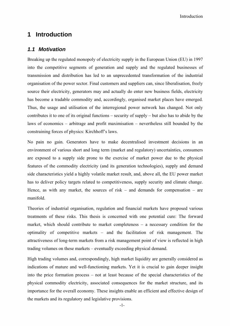
1.1 Motivation
Breaking up the regulated monopoly of electricity supply in the European Union (EU) in 1997
into the competitive segments of generation and supply and the regulated businesses of
transmission and distribution has led to an unprecedented transformation of the industrial
organisation of the power sector. Final customers and suppliers can, since liberalisation, freely
source their electricity, generators may and actually do enter new business fields, electricity
has become a tradable commodity and, accordingly, organised market places have emerged.
Thus, the usage and utilisation of the interregional power network has changed. Not only
contributes it to one of its original functions – security of supply – but also has to abide by the
laws of economics – arbitrage and profit maximisation – nevertheless still bounded by the
constraining forces of physics: Kirchhoff’s laws.
No pain no gain. Generators have to make decentralised investment decisions in an
environment of various short and long term (market and regulatory) uncertainties, consumers
are exposed to a supply side prone to the exercise of market power due to the physical
features of the commodity electricity (and its generation technologies), supply and demand
side characteristics yield a highly volatile market result, and, above all, the EU power market
has to deliver policy targets related to competitiveness, supply security and climate change.
Hence, as with any market, the sources of risk – and demands for compensation – are
manifold.
Theories of industrial organisation, regulation and financial markets have proposed various
treatments of these risks. This thesis is concerned with one potential cure: The forward
market, which should contribute to market completeness – a necessary condition for the
optimality of competitive markets – and the facilitation of risk management. The
attractiveness of long-term markets from a risk management point of view is reflected in high
trading volumes on these markets – eventually exceeding physical demand.
High trading volumes and, correspondingly, high market liquidity are generally considered as
indications of mature and well-functioning markets. Yet it is crucial to gain deeper insight
into the price formation process – not at least because of the special characteristics of the
physical commodity electricity, associated consequences for the market structure, and its
importance for the overall economy. These insights enable an efficient and effective design of
the markets and its regulatory and legislative provisions.

Introduction
-2-
1.2 Core research questions
This thesis analyses electricity forward and futures markets. Specifically it assesses the price
formation in these markets. Key objectives are to gain insights on major price and risk drivers
and to conclude on market efficiency. In particular, the following questions are addressed:
1. How are expectations formed in long-term markets?
2. What are the drivers of futures and forward prices?
3. What is the effect of trading of risk averse market actors on the futures-spot bias?
4. How do market structure and supply and demand shocks affect risk assessment and
market outcomes?
5. What, in turn, are the determinants of the forward premium?
6. What are the implications for market efficiency?
1.3 Methodology
Some of the above questions will be assessed by a review of the theoretical literature and by a
simple analytical equilibrium modelling approach. Most of this thesis is, however, concerned
with empirical analyses of the two main European power markets: The Central-Western
European and the Scandinavian power market. Both reduced-form regression and vector
autoregression models will be applied throughout this thesis.
1.4 Structure
The remainder or this thesis is structured as follows:
The following Chapter 2 unfolds the research problem. It briefly summarises the electricity
liberalisation process in the EU with a focus on the regulatory provisions, discusses and
reviews economic theory with respect to the price formation in liberalised power markets.
Thereby, it focuses on the pricing in forward markets and different theoretical and
methodological approaches. Then the social function of forward markets is discussed and a
simple two-stage equilibrium model is introduced. This model focuses on the price risk
management using forward contracts and explains stylised facts with respect to the emergence
of the futures-spot bias.
Chapters 3, 4 and 5 contain the specific empirical analyses mentioned above. These analyses
answer distinct though interlinked research questions. Common background information to all
analyses is provided in Chapter 2. In each case chapters 3 to 5 contain a detailed motivation
and introduction, describe the specific methodological approach and analysed data, present

Introduction
-3-
results and draw corresponding conclusions. Chapter 3 analyses the price formation in year-
ahead futures markets, Chapter 4 discusses the links between spot prices and futures prices of
different maturities and Chapter 5 assesses the drivers of the forward premium.
Overall conclusions from the analyses are drawn in Chapter 6. Appendix A contains an
additional robustness analysis of the model of the ex post forward premium presented in
Chapter 5. Appendix B dynamises a sub analysis of Chapter 5. Appendix C derives the
forward market equilibrium presented in section 2.3.2. Finally, Appendix D describes the
classical Cournot duopoly solution.
Liberalisation, price formation and risk management
-4-
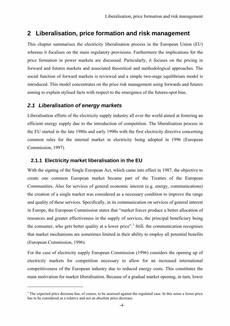
2 Liberalisation, price formation and risk management
This chapter summarises the electricity liberalisation process in the European Union (EU)
whereas it focalises on the main regulatory provisions. Furthermore the implications for the
price formation in power markets are discussed. Particularly, it focuses on the pricing in
forward and futures markets and associated theoretical and methodological approaches. The
social function of forward markets is reviewed and a simple two-stage equilibrium model is
introduced. This model concentrates on the price risk management using forwards and futures
aiming to explain stylised facts with respect to the emergence of the futures-spot bias.
2.1 Liberalisation of energy markets
Liberalisation efforts of the electricity supply industry all over the world aimed at fostering an
efficient energy supply due to the introduction of competition. The liberalisation process in
the EU started in the late 1980s and early 1990s with the first electricity directive concerning
common rules for the internal market in electricity being adopted in 1996 (European
Commission, 1997).
2.1.1 Electricity market liberalisation in the EU
With the signing of the Single European Act, which came into effect in 1987, the objective to
create one common European market became part of the Treaties of the European
Communities. Also for services of general economic interest (e.g. energy, communications)
the creation of a single market was considered as a necessary condition to improve the range
and quality of these services. Specifically, in its communication on services of general interest
in Europe, the European Commission states that “market forces produce a better allocation of
resources and greater effectiveness in the supply of services, the principal beneficiary being
the consumer, who gets better quality at a lower price”.1 Still, the communication recognises
that market mechanisms are sometimes limited in their ability to employ all potential benefits
(European Commission, 1996).
For the case of electricity supply European Commission (1996) considers the opening up of
electricity markets for competition necessary to allow for an increased international
competitiveness of the European industry due to reduced energy costs. This constitutes the
main motivation for market liberalisation. Because of a gradual market opening, in turn, lower
1 The expected price decrease has, of course, to be assessed against the regulated case. In this sense a lower price has to be considered as a relative and not an absolute price decrease.

Liberalisation, price formation and risk management
-5-
prices should also result for household consumers. The communication does not call for
privatisation of the energy sector. Instead, it focuses on the creation of competitive integrated
markets.
The restructuring of the electricity sector in the EU was finally triggered by the Directive
96/92/EC of the European Parliament and of the Council concerning common rules for the
internal market in electricity. Specifically, this directive contained three major provisions
(European Commission, 1997):
Regulating a minimum level of separation (unbundling) of the network (transmission
and distribution grid):
The formerly vertically electricity supply businesses had to separate their transmission
and distribution activities from generation and supply by means of unbundling of
accounts. In general, unbundling is of crucial importance in order to avoid possible
distortion of competition, discrimination and cross subsidies between different
segments of the supply chain (Haas et al., 2009).
Specification of network access models:
The directive foresaw two forms of third party access, negotiated or regulated, as well
as a single buyer procedure.
Opening up of former supply monopolies to allow eligible customers free choice of
their suppliers:
First, large customers with an annual consumption 40 GWh were eligible to choose
their supplier. This consumption limit was gradually decreased to 9 GWh six years
after the directive entered into force.
As recognised by European Commission (2007a) the minimum requirements set out by the
directive resulted in a diverse implementation and, hence, in considerable differences
regarding the level of market opening among the Member States. Furthermore, these
minimum legal requirements were not sufficient for implementing truly competitive markets.
Hence, a follow up directive2 containing stricter rules and responsibilities for the electricity
supply industry – and also for national authorities – entered into force in 2003 (European
Commission, 2003):
2 Directive 2003/54/EC of the European Parliament and of the Council. Official Journal of the European Union L176/37.
Liberalisation, price formation and risk management
-6-
Unbundling:
In addition to the unbundling of accounting and management the directive called for
legal unbundling. Hence, the transmission and distribution systems must be operated
through legally separate entities.
Network access:
Access to the system must be organised through a regulated third party access based
on published, objective and non discriminating tariffs monitored and methodologically
set by a regulatory authority.
Market opening:
The provisions pursued full market opening with non-household customers being
eligible from July 2004 and household customers from July 2007 on.
However, European Commission (2007b) questioned that, even after the second directive had
been implemented, electricity prices were the result of a truly competitive market
environment. Furthermore, insufficient unbundling provisions, discriminated third party
network access and lacking regulatory competences were observed. Considering this
unsatisfying process of achieving the internal market in electricity a third directive was set in
force in 2009 – yet again containing stricter rules. These rules have to be implemented in
national legislation by 2011. The most important provisions concern the unbundling of
integrated utilities (European Commission, 2009):
Unbundling:
The new directive calls for ownership unbundling as the preferred way to remove non-
competitive incentives of integrated incumbents. Possible alternatives to ownership
unbundling are the independent transmission system operator (ISO) which has control
over the network but ownership retains at the integrated utility and the independent
transmission operator (ITO) where the ownership and control of the network retain
within the integrated company subject to stricter regulation and oversight.
Furthermore, the competences and tasks of national regulators are increased and
provisions to stipulate cross border trade and investments are reinforced.
Liberalisation of the sector clearly effects the price formation of the commodity electricity. In
the former pre-liberalised times prices were regulated and equalled the average costs of power
generation. The next section will discuss price formation in liberalised markets.
Liberalisation, price formation and risk management
-7-
2.1.2 Price formation in liberalised electricity markets 3
In a competitive power market the price of electricity on the wholesale market is determined
by the generation costs of the marginal technology; that is the short run marginal costs of the
most expensive plant needed to meet demand. The price equals the so called system marginal
costs.4
The short run marginal costs mainly consist of the costs for input fuels (e.g. natural gas) and
CO2 certificates and to a lesser extent of other variable costs (e.g. operation and maintenance
cost). In this thesis, without affecting the results of the analysis in the following chapters,
short run marginal costs of different power plant technologies are modelled by considering
fuel and CO2 costs only.
When the generation capacity Q of all power plants in an electricity market is ordered by
short run generation costs c the total supply curve results. Since in a first approximation the
individual generation technologies have constant marginal costs until their capacity limit the
total supply curve is a stepped and discontinuous function of total capacity. As the utilisation
of the power plant park increases, typically, the supply curve is steeply increasing since the
individual plants eventually rely on more expensive fuels and are characterised by a
decreasing efficiency. Figure 2.1 shows a stylised supply curve where the generation costs are
plotted against the generation capacity. Typically run of river hydro power plants are
characterised by generation costs close to zero, followed by nuclear power plants, lignite, gas
and coal fired plants with oil fired plants usually constituting the most expensive generation
technologies.
The equilibrium electricity price is finally determined by the intersection of the supply and the
demand curve. As electricity demand can, in the short-term, be modelled as being inelastic to
price resulting in a vertical demand curve, competitive electricity markets can be modelled by
minimising the total generation costs to meet a given demand. Figure 2.1 illustrates price
formation in a competitive power market for two different demand levels (low, high).
3 This section is based on Haas, Redl and Auer (2009). 4 For a detailed description of price formation in liberalised electricity markets see, e.g., Stoft (2002).
Liberalisation, price formation and risk management
-8-
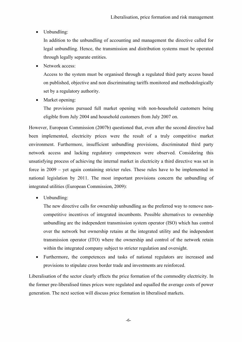
Figure 2.1. Price formation in a competitive electricity market. For the low and high demand case the wholesale prices, Plow and Phigh respectively, equals system marginal costs. That is, the short run generation costs of the most expensive plant needed to meet demand.
The intersection of supply and demand in Figure 2.1 implies that the last power plant type
needed to meet demand is utilised partly only. All technologies with lower generation costs
operate at maximum capacity. As supply and demand curves change over time (e.g. due to
seasonal factors or input price fluctuations) wholesale prices are characterised by volatile and
seasonal patterns.
This principle of system marginal cost pricing is, for example, mirrored in the concept of
uniform pricing auctions of organised wholesale electricity markets where all generators
needed to meet demand receive the clearing price. The difference between this price and the
individual generation costs is the contribution margin which allows for the coverage of fixed
costs. Summing this contribution margin for all operating generators yields the producer
surplus.5
2.1.3 Price formation in electricity forward markets
This thesis is concerned with price formation in futures/forward markets. That is, markets
where price formation and delivery are distinct. Hence, delivery is deferred. Delivery can take 5 There is a lively debate whether producers can recover their fixed investment costs in a fully liberalised and competitive power market. This thesis does not touch upon this issue. However, it should be pointed out that new power plants are characterised by high efficiencies and – within their load segment – should rarely constitute the marginal plant. In the long term the equilibrium price on a liberalised competitive power market equals the long run marginal costs of new power plants. For a discussion see Stoft (2002).
P, c
Q
Plow
Phigh
Liberalisation, price formation and risk management
-9-
place up to years after the corresponding prices where agreed on the market. Clearly, this
brings about complications in the price formation process. The above chapter, however, has
not considered these specificities. Instead, I implicitly assumed a generally effective price
formation process for both short term markets – also termed as spot markets – and long term
futures or forward markets. This corresponds to the presumption of risk neutral market actors
forming rational expectations in a competitive environment. This section therefore shows,
given these assumptions, that prices on short and long term markets are equal. The following
chapters, however, will relax these conjectures.
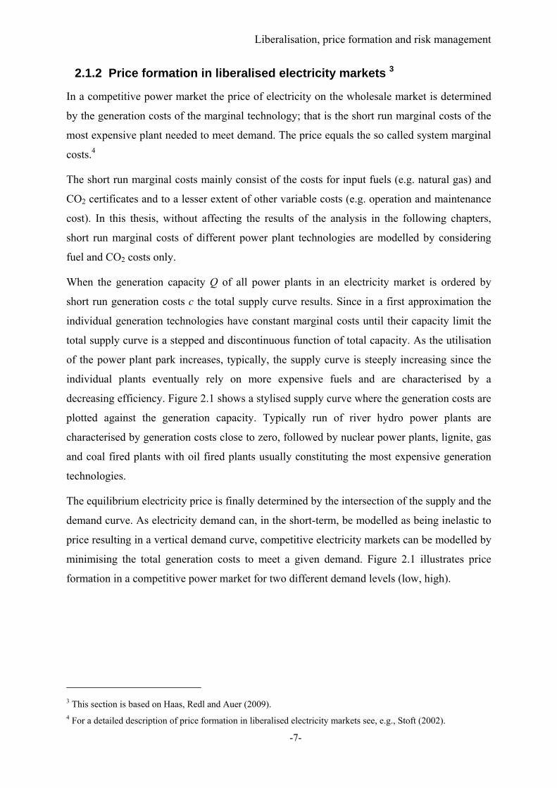
Figure 2.2 depicts the price convergence. In a risk neutral and competitive environment
rational market actors will, in equilibrium, agree on the forward price F based on the
intersection of the forecast of future (price inelastic) electricity demand Qs and the expected
upward sloping supply curve. This price equals the expected future spot price S when Qs and
the corresponding supply will finally materialise. The traded volume on the forward market
QF corresponds to this expected demand E(Qs). Random shocks causing deviations of Qs from
E(Qs) cause similar deviations of S from F (Borenstein et al., 2008). Given the above
assumptions, these deviations would have an expected value of zero. Any systematic price
differences would be eliminated by arbitrageurs buying in the cheaper and selling in the more
expensive market. These additional trading volumes would cause price convergence.
Figure 2.2. Equilibrium of forward and expected spot prices. Source: Borenstein et al. (2008)
Within the wider context of the financial behaviour of energy derivatives economic theory
provides two main approaches for pricing forward contracts. The first is dating back to Kaldor
(1939) where current spot prices, interest rates, storage costs and a convenience yield are used
to determine a no-arbitrage condition between spot and futures prices:
Pric
e
Q
Ft,T
Pric
e
Q
E(ST)
E(Qs) QF=E(Qs)
Liberalisation, price formation and risk management
-10-
))((,
tTcysrtTt eSF (2.1)
where Ft,T is the futures price at time t for delivery in T, St is the spot price at time t, r is a
constant interest rate, s are storage costs and cy is the convenience yield obtained from
holding the physical commodity.6 If the futures price deviated from this relationship,
arbitrageurs could secure riskless profits. More specifically, arbitrageurs would buy in the
cheaper market and sell in the more expensive market. As more market participants become
aware of this opportunity, arbitrage would be eliminated due to induced changes of the
demand and supply for spot and forward products.
However, the characteristics of electricity render its forward price formation rather special.
The most crucial aspect is the nonstorability of power which precludes the above classic cost
of carry equilibrium of spots and forwards. This nonstorability is amplified by the necessity of
an exact match of supply and demand in order to guarantee stability of the electricity
system.7,8 Instead, expanding the price formation process depicted in Figure 2.2, it is usual to
consider equilibrium in expectations and risk aversion (Keynes, 1930) amongst agents with
heterogeneous needs for hedging spot price uncertainty. The forward price Ft,T quoted at time
t for delivery at time T is thereby viewed as being determined as the expected spot price E(ST)
plus an ex ante forward premium FPt,T (Redl and Bunn, 2010):
TtTTt FPSEF ,, )( (2.2)
Expected spot prices reflect market participants’ expectations of fundamental supply and
demand conditions during the delivery period of the forward contract (as depicted in Figure
2.2). Differences between forward and expected future spot prices are then a compensation for
bearing the price risk (Bessembinder 1992, Bessembinder and Lemmon 2002, Longstaff and
Wang 2004). The forward premium is thereby considered the net hedging cost of risk averse
producers, retailers or other market participants.9,10 In essence, the forward premium
6 See e.g. Telser (1958) for the concept of convenience yield for futures pricing. 7 From an economic point of view the non-storability implies high storage costs yielding – according to equation (2.1) – high futures prices. 8 Nonetheless, the cost of carry approach is used in the electricity literature (see e.g. Clewlow and Strickland (2000), Stoft et al. (1998) on arbitrage pricing of electricity futures). 9 Fama (1984) states that equation (2.2) is simply a definition of the premium. Section 2.3 will present a model describing the emergence of this premium. 10 The terms “forward premium” and “risk premium” are used interchangeably in many papers. However, it is important to stick to the definition: The risk premium is the negative of the forward premium. Hence, the forward premium is the difference between the futures price and the expected spot price whereas the risk premium is simply the opposite.
Liberalisation, price formation and risk management
-11-
constitutes the costs of a hedge in order to insure a fixed price ahead of the delivery (i.e. the
futures price).
Besides equilibrium approaches for forward price modelling stochastic models are frequently
applied to determine the magnitude of inherent market risk (See Weron (2008), Kolos and
Ronn (2008), Benth and Koekebakker (2008) and the references therein). In this thesis a
structural approach for modelling forward prices is employed to study the relationship
between forward and spot prices and gain insights on fundamental influence factors.
Testing the expectations theory challenges the empirical researcher. Prices, clearly, can only
be observed ex post. However, equation (2.2) contains two non-observable ex ante terms.
Hence, assessing both the forecasting power of forward prices (i.e. testing the consistency of
expected prices) and the premium (i.e. testing the significance and magnitude of the price of
risk) is a highly interlinked and intriguing problem. Still, equation (2.2) also presents two
natural alternatives circumventing this inference problem. First, an ex ante spot price model
can capture the price expectation formation allowing the deduction of the premium. Second,
expanding equation (2.2) by the realised spot price allows a direct estimation of the premium.
Some words of caution: Relocating the inference problem does not, however, resolve all
empirical challenges. Chapter 5 will present a detailed motivation why the latter of the two
above mentioned alternatives is, nevertheless, a careful approach paving the way for relevant
and robust conclusions on the price formation in electricity forward markets.
A remark on nomenclature is overdue: Throughout this thesis the terms futures and forwards
are used interchangeably. However, these two types of contracts differ – most importantly in
terms of their settlement. Forward contracts, which are typically settled with physical delivery
of the underlying commodity, yield cash flows (i.e. forward price times quantity) at the
maturity date. In contrast, futures contracts, which are typically settled financially and traded
at organised exchanges, comprise cash flows during the remaining time to maturity according
to the change in the market value of the contract (i.e. the price changes of the contract). Since
futures prices converge to the spot price due to arbitrage reasons this continuous settlement
causes that e.g. for the purchase of the commodity at maturity simply the prevailing spot price
has to be paid (Cox et al., 1981). In reality this daily settlement is paid out of a deposit (the
margin) traders are required to leave at the exchanges. Cox et al. (1981) show that for

Liberalisation, price formation and risk management
-12-
constant interest rates futures and forward prices are, in fact, equal. Hence, this thesis
implicitly assumes non-stochastic interest rates when referring to futures or forwards.11
2.2 The social function of forward markets
Forward markets deliver two main functions in an economy: They provide and aggregate
information about future prices and allow for hedging price risks (Newbery and Stiglitz,
1981). That is, they contribute to market completeness – which is a necessary condition for
competitive markets to be Pareto optimal – and facilitate risk management and risk transfer.12
The current electricity futures price is the market’s best estimate (adjusted for forward
premia) of the future price of this commodity. This, in turn, provides information to market
participants and allows an adjustment of (future) production and consumption decisions.
However, as pointed out by Newbery and Stiglitz (1981), information on the market may be
biased due to conflicting benefits of privately versus socially available information.
The most important function of futures markets is the facilitation of risk management
(hedging) of risk averse market actors. For example, a generator can sell power forward for
future delivery and effectively lock in a fixed sale price at the time of the forward trade.
Clearly, this illustration shows that forward markets provide a means for hedging price risk,
whereas the risk of demand fluctuations cannot be cured by forwards. To also hedge the
quantity risk13 more sophisticated derivatives, namely option contracts, need to be entered by
the respective generator.14 The next section will show the effects of hedging on the price
formation and profit distribution using an analytical model.
11 Given the short time to delivery of the considered contracts a constant interest rate may indeed be a safe assumption. 12 With the work of Allaz (1992) another social function of forward markets entered the economic debate: The strategic role of forwards in an oligopolistic market environment and its (positive) effect on efficiency. However, this result has been questioned by the theoretical literature and not been resolved by empirical studies. Hence this ambiguous function is not treated in this section. Instead, I refer to section 5.2.1.1 for a discussion of the strategic effects of forward markets and section 5.6 for an empirical analysis. 13 Similarly, unexpected generation unit outages cause supply fluctuations representing another component of quantity risk. 14 This thesis, however, is primarily concerned with the treatment of futures markets and, hence, the assessment of the facilitation of price risk management.
Liberalisation, price formation and risk management
-13-
2.3 Price risk management using forward contracts: A simple
analytical model
This section is concerned with the effects of forward trading on the profit distribution of risk
averse power generators in an uncertain market environment. The model is kept as simply as
possible in order to focus on the risk hedging function of forward markets. For more
elaborated models see, e.g., Danthine (1978), Anderson and Danthine (1981), Newbery and
Stiglitz (1981), and Bessembinder and Lemmon (2002).15
The model contains NP risk averse producers acting competitively in the spot and forward
market. The total cost function of each identical supplier i is a function of the individual
output QPi and fixed costs FC and is set to . The passive demand side is
modelled via an inelastic demand function with expected mean demand QD which is normally
distributed with demand variance σD2. Uncertainty about demand is resolved when the spot
market clears.
2.3.1 Spot market equilibrium
Taking into account the previously agreed forward positions the ex post profit πPi of producer
i equals
(2.3)
where PW is the wholesale spot price, PF is the forward price, and QPiW and QPi
F denote the
quantities sold by producer i on the spot and forward market respectively. Clearly, generator
i’s total physical production QPi is the sum of QPiW and QPi
F. The first order condition yields
the profit maximising quantity sold in the spot market by producer i:16
0 (2.4)
(2.5)
Given that forward contracts are in sum zero net supply17 and equating total production to
total demand yields the equilibrium spot price:
15 The presented model keeps the notation of Bessembinder and Lemmon (2002) as much as possible since their model is discussed in detail in section 5.2.1.2. 16 It is easy to verify that the second order condition for a maximum is fulfilled.
17 ∑ ∑ 0

Liberalisation, price formation and risk management
-14-
(2.6)
2.3.2 Forward market equilibrium 18
Participants on the forward market include the producers and NS risk averse speculators j who
do not take a physical position in the spot market.19 Market actors are assumed, for simplicity,
to maximise the well-known mean-variance utility function:20
, , , (2.7)
where E(πi,j) is the expected value of the profit of generator i and speculator j respectively and
Var(πi,j) is the variance of the respective profit distribution.21 Using (2.5) and the properties of
variances and covariances22 yields the following function for expected utility for producer i23
, (2.8)
and for speculator j24
(2.9)
The first order conditions give the profit maximising quantity sold (or bought) in the forward
market:25
18 For a stepwise derivation of the forward market equilibrium see Appendix C. 19 For simplicity, the model just includes producers and speculators in the forward stage. More sophisticated models may also include retailers (e.g. Bessembinder and Lemmon (2002)). Since the aim of this section is to point out the risk hedging function of forward markets the results would not be altered if retailers where included in the model. Clearly, speculators could be considered to be part of the total system demand. Hence, a passive demand side representation is taken into account in the spot market stage. 20 This utility function constitutes a strong assumption. Particularly, returns need to be distributed normally and agents are assumed to maximise utility functions with constant absolute risk aversion. See Newbery and Stiglitz (1981) and Newbery (1988) for a detailed discussion of the limitations of the mean variance approach. Clearly, it seems reasonable that risk averse agent’s are also concerned with the volatility of the expected profits – measured in this case by the variance of profits. The linear form of the above model yields normality of the return distribution. 21 In this model market participants form rational expectations. Hence, they know the true distribution of power demand. This is a strong assumption. Nevertheless, this model formulation allows best focusing on the hedging part of the forward bias. 22 Var(x)=E(x2)-E2(x) and Cov(x,y)=E(xy)-E(x)E(y).
23 and ,
24 The speculator maximises .
25 Again, it is easy to verify that the second order conditions for a maximum are fulfilled.

Liberalisation, price formation and risk management
-15-
, (2.10)
for the producer and
(2.11)
for the speculator. Since forward markets are in sum zero net26 supply the market clearing
forward price can be calculated:
, (2.12)
Inserting (2.12) in (2.10) and (2.11) finally yields
, (2.13)
and
, (2.14)
2.3.3 Simulation of market equilibria
In the following the main results of the above sections are simulated by normalising demand
QD to 100 MWh, setting NP and NS to 20 and 10 respectively, A to 0.5, a to 4 €/MWh2 and FC
to 0. The standard deviation of demand σD is varied between 0 and 10 (i.e. up to 10% of mean
demand). Given these assumptions the expected value of the spot market wholesale price PW
equals 20 €/MWh.
If producers cannot hedge their production on the forward market expected profits are solely
determined by spot market transactions. In this case, setting the demand standard deviation σD
to 5, the expected value of the profit E(πPi) of producer i equals 50 € and the standard
deviation of expected profits equals 5 €.27 If producers can hedge their transactions on the
spot market, which by definition of risk averse market actors is what they do, the expected
value of the profit E(πPi) of producer i reduces to 47.3 €. On the other hand the standard
deviation of expected profits reduces to 3.3 €.28 The forward price PF is downward biased and
amounts to 18.3 €/MWh. The price difference to the spot price constitutes the cost of the
26 ∑ ∑ 0
27 The absolute numbers in this example are not of importance. Instead, the relative performance of the spot market and the market with spot and forward contracts matters. 28 This results from the trade-off of the mean-variance maximisation.
Liberalisation, price formation and risk management
-16-
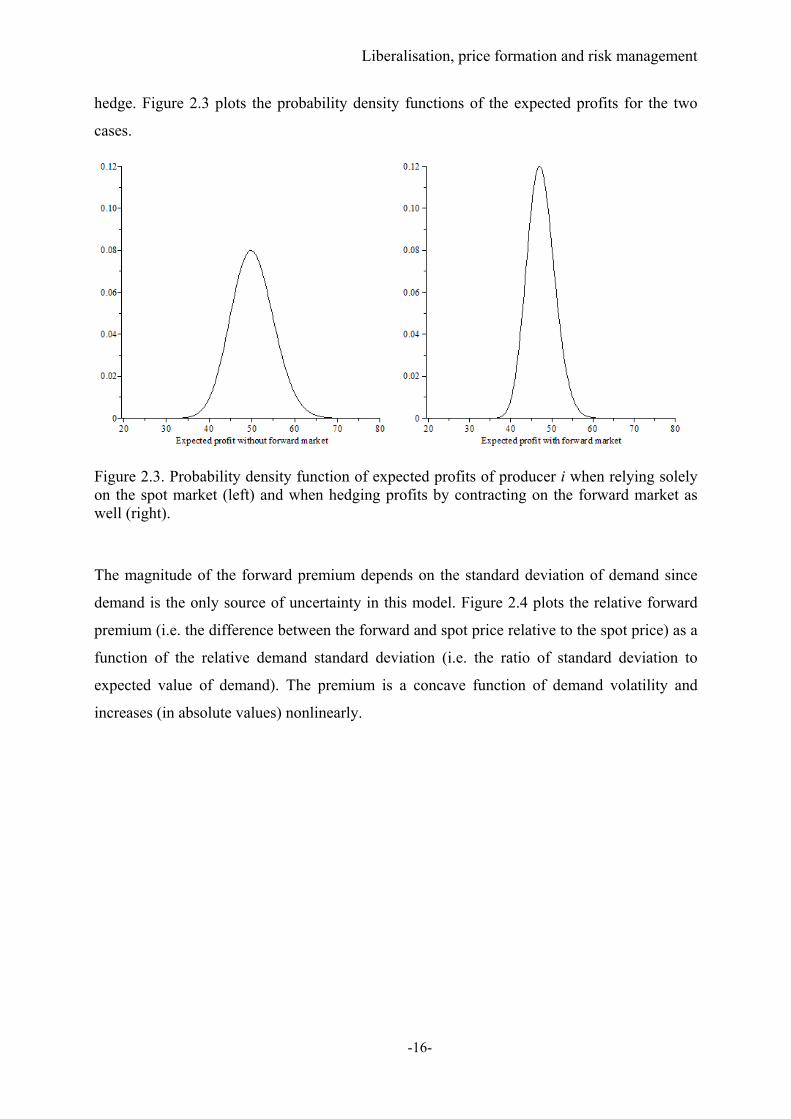
hedge. Figure 2.3 plots the probability density functions of the expected profits for the two
cases.
Figure 2.3. Probability density function of expected profits of producer i when relying solely on the spot market (left) and when hedging profits by contracting on the forward market as well (right).
The magnitude of the forward premium depends on the standard deviation of demand since
demand is the only source of uncertainty in this model. Figure 2.4 plots the relative forward
premium (i.e. the difference between the forward and spot price relative to the spot price) as a
function of the relative demand standard deviation (i.e. the ratio of standard deviation to
expected value of demand). The premium is a concave function of demand volatility and
increases (in absolute values) nonlinearly.
Liberalisation, price formation and risk management
-17-
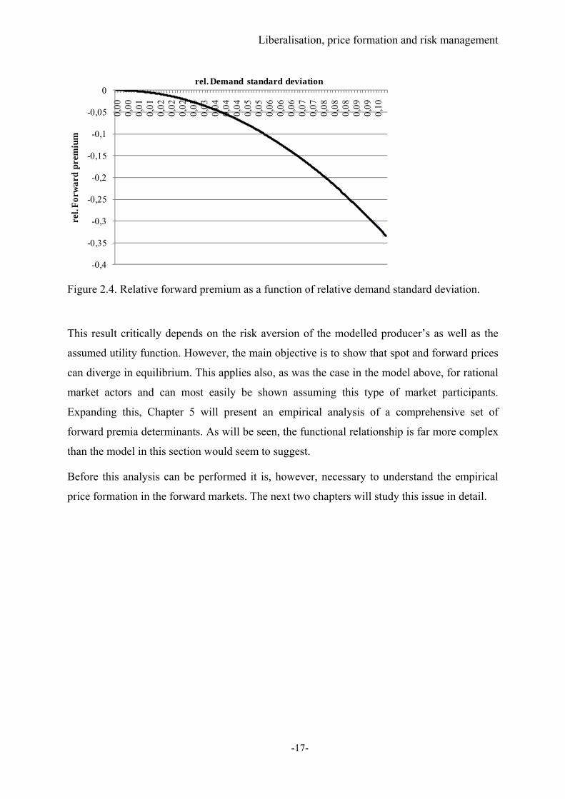
Figure 2.4. Relative forward premium as a function of relative demand standard deviation.
This result critically depends on the risk aversion of the modelled producer’s as well as the
assumed utility function. However, the main objective is to show that spot and forward prices
can diverge in equilibrium. This applies also, as was the case in the model above, for rational
market actors and can most easily be shown assuming this type of market participants.
Expanding this, Chapter 5 will present an empirical analysis of a comprehensive set of
forward premia determinants. As will be seen, the functional relationship is far more complex
than the model in this section would seem to suggest.
Before this analysis can be performed it is, however, necessary to understand the empirical
price formation in the forward markets. The next two chapters will study this issue in detail.
-0,4
-0,35
-0,3
-0,25
-0,2
-0,15
-0,1
-0,05
0
0,00
0,00
0,01
0,01
0,02
0,02
0,02
0,03
0,03
0,04
0,04
0,04
0,05
0,05
0,06
0,06
0,06
0,07
0,07
0,08
0,08
0,08
0,09
0,09
0,10
rel.
For
war
d pr
emiu
mrel. Demand standard deviation
Price formation in electricity forward markets: The case of year-ahead futures prices
-18-
3 Price formation in electricity forward markets: The case
of year-ahead futures prices 29
Due to the high relevance of long-term electricity markets for risk management reasons
pointed out in the previous chapter the determination of influence factors on the price
formation on these markets is of great importance. For pricing of these contracts an important
fact concerns the non-storability of electricity. In this case, according to economic theory,
forward prices are related to expected spot prices which are built on fundamental market
expectations. Therefore, in this chapter the crucial impact parameters on year-ahead forward
electricity prices are assessed by an empirical analysis of electricity prices at two of the
biggest European power exchanges: the European Energy Exchange (EEX) based in Leipzig,
Germany, and the Nord Pool Power Exchange, based in Oslo, Norway.30 The analysis is
based on considerations of expectation formation of market participants. Specifically, reduced
form regression models aim to give insights on the expectation and price formation. As will
be seen, the price formation in the considered markets is influenced by historic spot market
prices yielding a biased forecasting power of long-term contracts.
This chapter proceeds as follows: The next section introduces the market setting and the
analysed data set. Section 3.2 focuses on an econometric analysis of year-ahead forward
prices. Finally, section 3.3 concludes.
3.1 Market setting and data analysis
The European electricity market is still characterised by several different price areas. Reasons
for this price divergence can be found, among others, in limited cross-border transmission
capacities (European Commission, 2005). In turn, varying generation conditions between
many Member States of the European Union result in different electricity wholesale price
levels. However, several regional electricity markets have emerged within the European
Union as some countries are not separated by permanent cross-border transmission capacity
bottlenecks causing prices to converge. Figure 3.1 summarises the status of the year 2009.
29 A concise version of this analysis has been published in Redl et al. (2009). 30 As mentioned the terms futures and forwards are used interchangeably in this thesis. Nevertheless, long-term contracts traded at the EEX are called futures whereas Nord Pool terms its contracts with delivery periods lasting at least one month forwards.
Price formation in electricity forward markets: The case of year-ahead futures prices
-19-
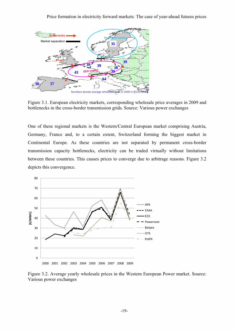
Figure 3.1. European electricity markets, corresponding wholesale price averages in 2009 and bottlenecks in the cross-border transmission grids. Source: Various power exchanges
One of these regional markets is the Western/Central European market comprising Austria,
Germany, France and, to a certain extent, Switzerland forming the biggest market in
Continental Europe. As these countries are not separated by permanent cross-border
transmission capacity bottlenecks, electricity can be traded virtually without limitations
between these countries. This causes prices to converge due to arbitrage reasons. Figure 3.2
depicts this convergence.
Figure 3.2. Average yearly wholesale prices in the Western European Power market. Source: Various power exchanges
Nord Pool market
43
37
39
64
3839
Bottlenecks
Market separation
39
39
35
38
Numbers denote average wholesale price in 2009 in [EUR/MWh]
0
10
20
30
40
50
60
70
80
2000 2001 2002 2003 2004 2005 2006 2007 2008 2009
[€/M
Wh]
APX
EXAA
EEX
Powernext
Belpex
OTE
PolPX
Price formation in electricity forward markets: The case of year-ahead futures prices
-20-
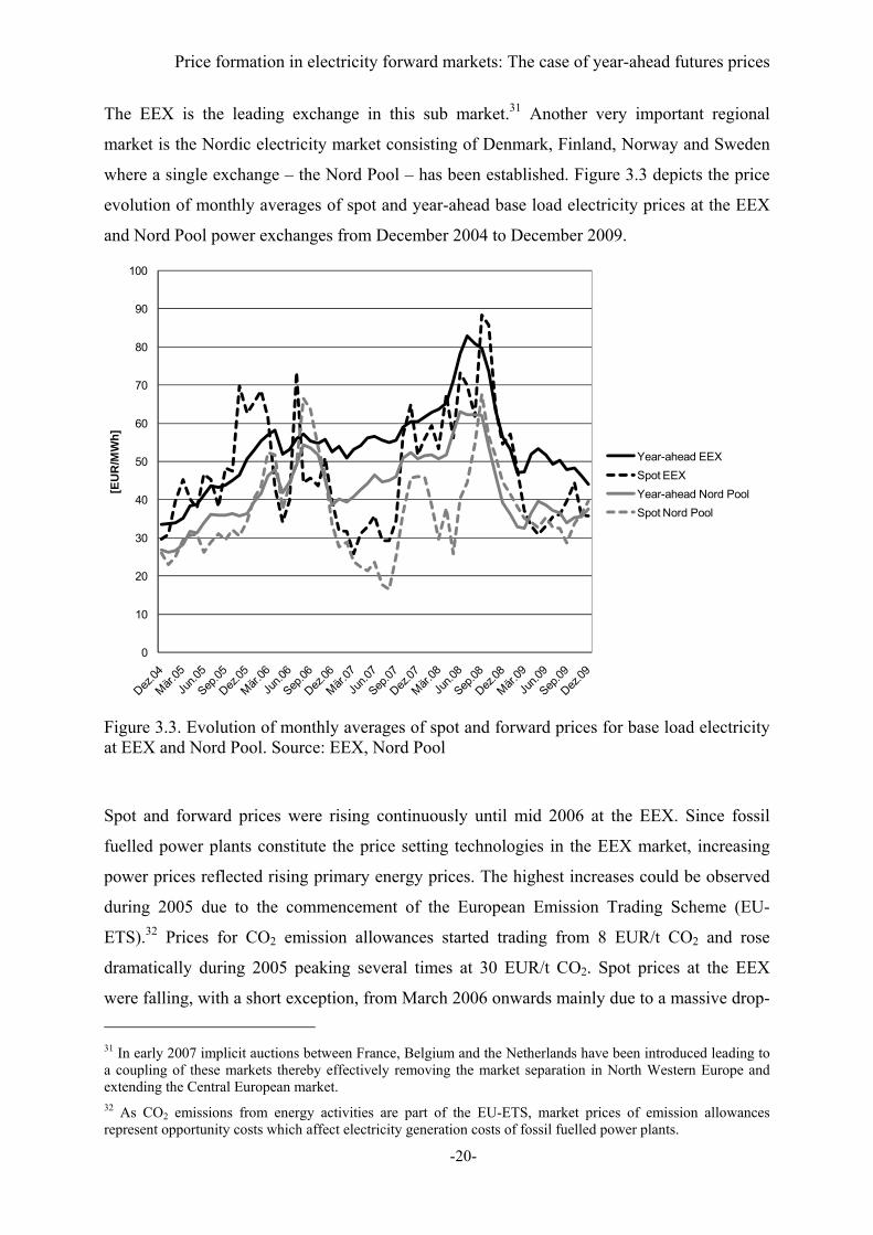
The EEX is the leading exchange in this sub market.31 Another very important regional
market is the Nordic electricity market consisting of Denmark, Finland, Norway and Sweden
where a single exchange – the Nord Pool – has been established. Figure 3.3 depicts the price
evolution of monthly averages of spot and year-ahead base load electricity prices at the EEX
and Nord Pool power exchanges from December 2004 to December 2009.
Figure 3.3. Evolution of monthly averages of spot and forward prices for base load electricity at EEX and Nord Pool. Source: EEX, Nord Pool
Spot and forward prices were rising continuously until mid 2006 at the EEX. Since fossil
fuelled power plants constitute the price setting technologies in the EEX market, increasing
power prices reflected rising primary energy prices. The highest increases could be observed
during 2005 due to the commencement of the European Emission Trading Scheme (EU-
ETS).32 Prices for CO2 emission allowances started trading from 8 EUR/t CO2 and rose
dramatically during 2005 peaking several times at 30 EUR/t CO2. Spot prices at the EEX
were falling, with a short exception, from March 2006 onwards mainly due to a massive drop-
31 In early 2007 implicit auctions between France, Belgium and the Netherlands have been introduced leading to a coupling of these markets thereby effectively removing the market separation in North Western Europe and extending the Central European market. 32 As CO2 emissions from energy activities are part of the EU-ETS, market prices of emission allowances represent opportunity costs which affect electricity generation costs of fossil fuelled power plants.
0
10
20
30
40
50
60
70
80
90
100
[EU
R/M
Wh
]
Year-ahead EEX
Spot EEX
Year-ahead Nord Pool
Spot Nord Pool
Price formation in electricity forward markets: The case of year-ahead futures prices
-21-
off in emission allowance prices. Still, year-ahead prices have maintained their high level
from early 2006 because of high gas and later on high (2008-) forward emission allowance
prices. In 2008 EEX spot prices again reached the level of the forward price due to a price
jump on the spot market for CO2 allowances when the second EU-ETS period started in
January 2008. Prices were falling from mid/end 2008 on due to falling primary energy prices
(mainly triggered by falling oil prices).
Nord Pool prices follow a different pattern. The Scandinavian power market is mainly
characterised by hydro and nuclear generation with 76% of total generation in 2007 stemming
from these two generation sources whereas hydro and nuclear generation corresponds to 59%
in the Central European sub market.33 In times of high hydro generation in Scandinavia only
highly efficient plants are needed to satisfy demand resulting in lower pool prices compared
to the EEX. Still, low hydro availability implying congested transmission grids and increased
generation in inefficient thermal power plants, causes prices soaring above EEX levels.
Compared to spot prices, year-ahead forward prices follow a less volatile regime for both
markets whereas Nordic prices are generally lower than their EEX counterparts due to the
mentioned differences in the power plant park structures. At first sight, spot and forward
prices show a higher correlation in the Scandinavian market most likely due to the high
amount of hydro storage capacity especially in Norway (see e.g. Gjolberg and Johnsen
(2001), and Botterud et al. (2002)).
Figure 3.4 shows crucial influence parameters for European forward electricity prices, namely
futures prices for hard coal (North-western Europe port prices – ARA ports), natural gas
(Zeebrugge hub), CO2 allowances (EUA) and year-ahead base load futures traded at the EEX
and Nord Pool. A positive relationship between CO2, natural gas and electricity futures as
well as a weak correlation between mainly stable coal and rising electricity futures quotations
can be observed.
33 See, e.g., Nordel (2008) and UCTE (2008) on detailed statistics about the considered markets.
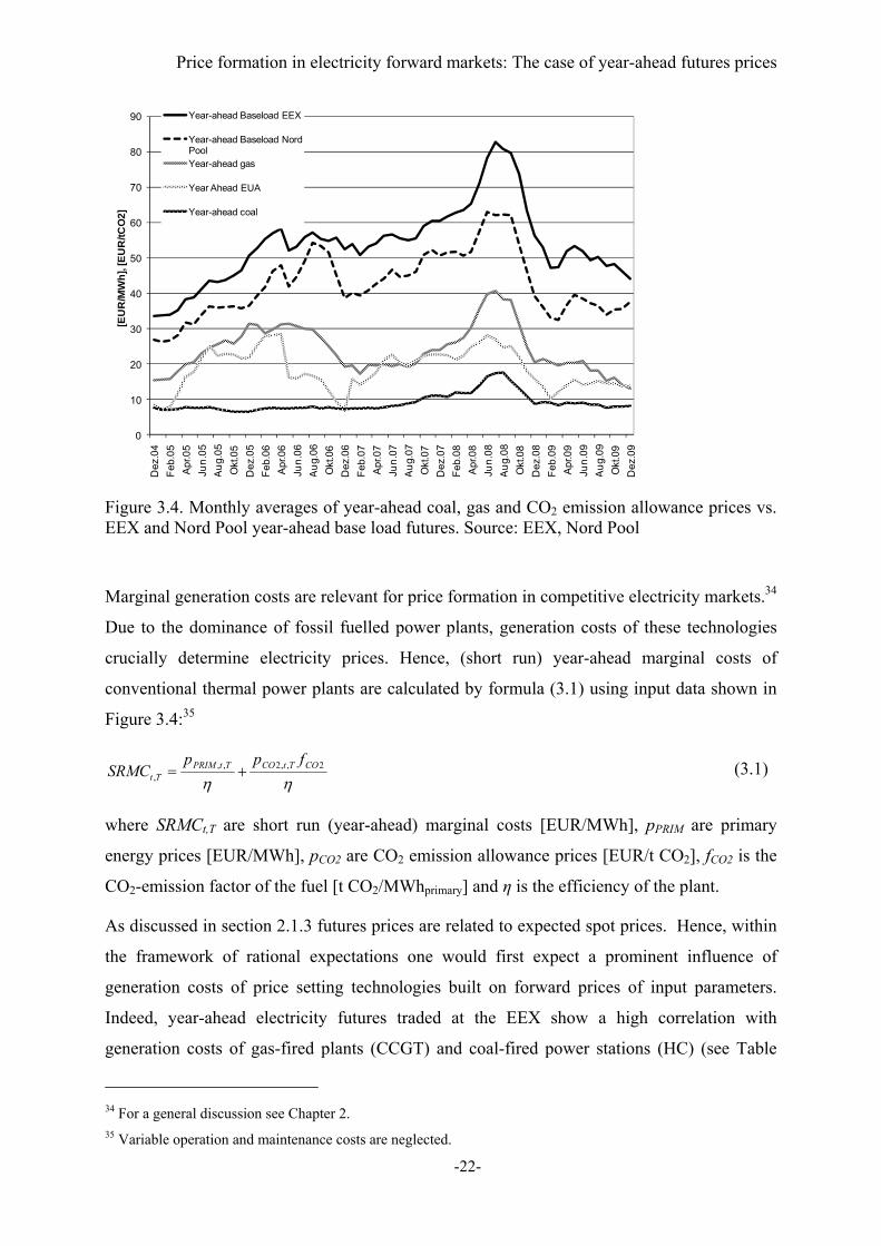
Price formation in electricity forward markets: The case of year-ahead futures prices
-22-
Figure 3.4. Monthly averages of year-ahead coal, gas and CO2 emission allowance prices vs. EEX and Nord Pool year-ahead base load futures. Source: EEX, Nord Pool
Marginal generation costs are relevant for price formation in competitive electricity markets.34
Due to the dominance of fossil fuelled power plants, generation costs of these technologies
crucially determine electricity prices. Hence, (short run) year-ahead marginal costs of
conventional thermal power plants are calculated by formula (3.1) using input data shown in
Figure 3.4:35
2,,2,,
,COTtCOTtPRIM
Tt
fppSRMC (3.1)
where SRMCt,T are short run (year-ahead) marginal costs [EUR/MWh], pPRIM are primary
energy prices [EUR/MWh], pCO2 are CO2 emission allowance prices [EUR/t CO2], fCO2 is the
CO2-emission factor of the fuel [t CO2/MWhprimary] and η is the efficiency of the plant.
As discussed in section 2.1.3 futures prices are related to expected spot prices. Hence, within
the framework of rational expectations one would first expect a prominent influence of
generation costs of price setting technologies built on forward prices of input parameters.
Indeed, year-ahead electricity futures traded at the EEX show a high correlation with
generation costs of gas-fired plants (CCGT) and coal-fired power stations (HC) (see Table
34 For a general discussion see Chapter 2. 35 Variable operation and maintenance costs are neglected.
0
10
20
30
40
50
60
70
80
90
De
z.0
4
Fe
b.0
5
Ap
r.05
Jun
.05
Au
g.0
5
Okt
.05
De
z.0
5
Fe
b.0
6
Ap
r.06
Jun
.06
Au
g.0
6
Okt
.06
De
z.0
6
Fe
b.0
7
Ap
r.07
Jun
.07
Au
g.0
7
Okt
.07
De
z.0
7
Fe
b.0
8
Ap
r.08
Jun
.08
Au
g.0
8
Okt
.08
De
z.0
8
Fe
b.0
9
Ap
r.09
Jun
.09
Au
g.0
9
Okt
.09
De
z.0
9
[EU
R/M
Wh
], [
EU
R/t
CO
2]
Year-ahead Baseload EEX
Year-ahead Baseload Nord PoolYear-ahead gas
Year Ahead EUA
Year-ahead coal

Price formation in electricity forward markets: The case of year-ahead futures prices
-23-
3.1). However, EEX year-ahead prices also show a high correlation with current spot prices
indicating adaptive expectation formation behaviour of market participants in the futures
market where the spot price serves as an estimator of year-ahead electricity prices.36,37 A
similar link between forward prices and generation costs of fossil fuelled plants prevails in the
Nordic market (see Table 3.1). An adaptive price formation component can also be observed
in this market given the correlation between forward and current spot prices. As mentioned
earlier, the high amount of reservoirs in the Nord Pool area can serve as an explanation.
Table 3.1. Correlation coefficients between monthly averages of EEX and Nord Pool year-ahead base load prices and explanatory variables from December 2004 to December 2009.
Correlation coefficient
EEX Nord Pool
Year-aheadBase t,T / SRMCCCGT_Zeebrugge t,T 0.74 0.75
Year-aheadBase t,T / SRMCHC_ARA t,T 0.86 0.81
Year-aheadBase t,T / Spot t 0.61 0.57
In the following, the year-ahead forward price at EEX and Nord Pool will be explained with
the abovementioned variables by performing econometric analyses.
3.2 A model for year-ahead electricity prices
Comparing the abovementioned variables to futures prices suggests that futures prices at both
exchanges are strongly influenced by both spot market prices and year-ahead generation costs
for CCGT and HC plants. Generation costs, determined from input prices shown in Figure 3.4
according to (3.1), represent fundamental explanatory variables of the model. To be able to
account for non-linear effects quadratic cost terms are included additionally. The current spot
price represents an explanatory variable to incorporate adaptive behaviour of market
participants into the model. All time series exhibit clear trends and thus must be considered to
represent non-stationary processes which is confirmed by unit root tests. As the hypothesis of
a cointegrated relationship has to be strongly rejected (by an Engle-Granger test with an ADF
36 Karakatsani and Bunn (2008) show that British spot prices are significantly influenced by lagged spot prices – this autoregressive price effect could indicate market inefficiency. 37 As will be discussed in chapters 4 and 5, a link in electricity spot and forward prices may emerge from a link in storable fuels serving as production inputs (coal and gas). Still, the correlation among the exogenous variables in (3.2) is low (about 20% for spots and generation costs) indicating a prominent influence of the spot price on the futures price itself.
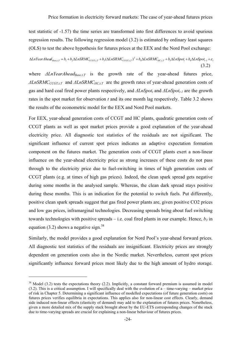
Price formation in electricity forward markets: The case of year-ahead futures prices
-24-
test statistic of -1.57) the time series are transformed into first differences to avoid spurious
regression results. The following regression model (3.2) is estimated by ordinary least squares
(OLS) to test the above hypothesis for futures prices at the EEX and the Nord Pool exchange:
tttTtHCTtCCGTTtCCGTTtBase LnSpotbLnSpotbLnSRMCbLnSRMCbLnSRMCbbdLnYearAhea 165,,42
,,3,,21,, )(
(3.2)
where ΔLnYearAheadBase,t,T is the growth rate of the year-ahead futures price,
ΔLnSRMCCCGT,t,T and ΔLnSRMCHC,t,T are the growth rates of year-ahead generation costs of
gas and hard coal fired power plants respectively, and ΔLnSpott and ΔLnSpott-1 are the growth
rates in the spot market for observation t and its one month lag respectively. Table 3.2 shows
the results of the econometric model for the EEX and Nord Pool markets.
For EEX, year-ahead generation costs of CCGT and HC plants, quadratic generation costs of
CCGT plants as well as spot market prices provide a good explanation of the year-ahead
electricity price. All diagnostic test statistics of the residuals are not significant. The
significant influence of current spot prices indicates an adaptive expectation formation
component on the futures market. The generation costs of CCGT plants exert a non-linear
influence on the year-ahead electricity price as strong increases of these costs do not pass
through to the electricity price due to fuel-switching in times of high generation costs of
CCGT plants (e.g. at times of high gas prices). Indeed, the clean spark spread gets negative
during some months in the analysed sample. Whereas, the clean dark spread stays positive
during these months. This is an indication for the potential to switch fuels. Put differently,
positive clean spark spreads suggest that gas fired power plants are, given positive CO2 prices
and low gas prices, inframarginal technologies. Decreasing spreads bring about fuel switching
towards technologies with positive spreads – i.e. coal fired plants in our example. Hence, b3 in
equation (3.2) shows a negative sign.38
Similarly, the model provides a good explanation for Nord Pool’s year-ahead forward prices.
All diagnostic test statistics of the residuals are insignificant. Electricity prices are strongly
dependent on generation costs also in the Nordic market. Nevertheless, current spot prices
significantly influence forward prices most likely due to the high amount of hydro storage.
38 Model (3.2) tests the expectations theory (2.2). Implicitly, a constant forward premium is assumed in model (3.2). This is a critical assumption. I will specifically deal with the evolution of a – time-varying – market price of risk in Chapter 5. Determining a significant influence of modelled expectations (of future generation costs) on futures prices verifies equilibria in expectations. This applies also for non-linear cost effects. Clearly, demand side induced non-linear effects (elasticity of demand) may add to the explanation of futures prices. Nonetheless, given a more detailed mix of the supply stack brought about by the EU-ETS corresponding changes of the stack due to time-varying spreads are crucial for explaining a non-linear behaviour of futures prices.
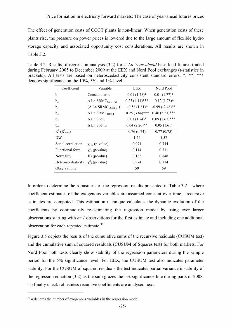
Price formation in electricity forward markets: The case of year-ahead futures prices
-25-
The effect of generation costs of CCGT plants is non-linear. When generation costs of these
plants rise, the pressure on power prices is lowered due to the large amount of flexible hydro
storage capacity and associated opportunity cost considerations. All results are shown in
Table 3.2.
Table 3.2. Results of regression analysis (3.2) for Δ Ln Year-ahead base load futures traded during February 2005 to December 2009 at the EEX and Nord Pool exchanges (t-statistics in brackets). All tests are based on heteroscedasticity consistent standard errors. *, **, *** denotes significance on the 10%, 5% and 1%-level.
Coefficient Variable EEX Nord Pool
b1 Constant term 0.01 (1.78)* 0.01 (1.77)*
b2 Δ Ln SRMCCCGT t,T 0.23 (4.11)*** 0.12 (1.78)*
b3 (Δ Ln SRMCCCGT t,T)2 -0.58 (1.81)* -0.99 (-2.48)**
b4 Δ Ln SRMCHC t,T 0.25 (3.64)*** 0.46 (5.23)***
b5 Δ Ln Spot t 0.03 (1.74)* 0.09 (2.67)***
b6 Δ Ln Spot t-1 0.04 (2.26)** 0.05 (1.61)
R2 (R2corr) 0.76 (0.74) 0.77 (0.75)
DW 1.24 1.57
Serial correlation χ212 (p-value) 0.071 0.744
Functional form χ21 (p-value) 0.114 0.311
Normality JB (p-value) 0.183 0.848
Heteroscedasticity χ25 (p-value) 0.974 0.314
Observations 59 59
In order to determine the robustness of the regression results presented in Table 3.2 – where
coefficient estimates of the exogenous variables are assumed constant over time – recursive
estimates are computed. This estimation technique calculates the dynamic evolution of the
coefficients by continuously re-estimating the regression model by using ever larger
observations starting with n+1 observations for the first estimate and including one additional
observation for each repeated estimate.39
Figure 3.5 depicts the results of the cumulative sums of the recursive residuals (CUSUM test)
and the cumulative sum of squared residuals (CUSUM of Squares test) for both markets. For
Nord Pool both tests clearly show stability of the regression parameters during the sample
period for the 5% significance level. For EEX, the CUSUM test also indicates parameter
stability. For the CUSUM of squared residuals the test indicates partial variance instability of
the regression equation (3.2) as the sum grazes the 5% significance line during parts of 2008.
To finally check robustness recursive coefficients are analysed next.
39 n denotes the number of exogenous variables in the regression model.
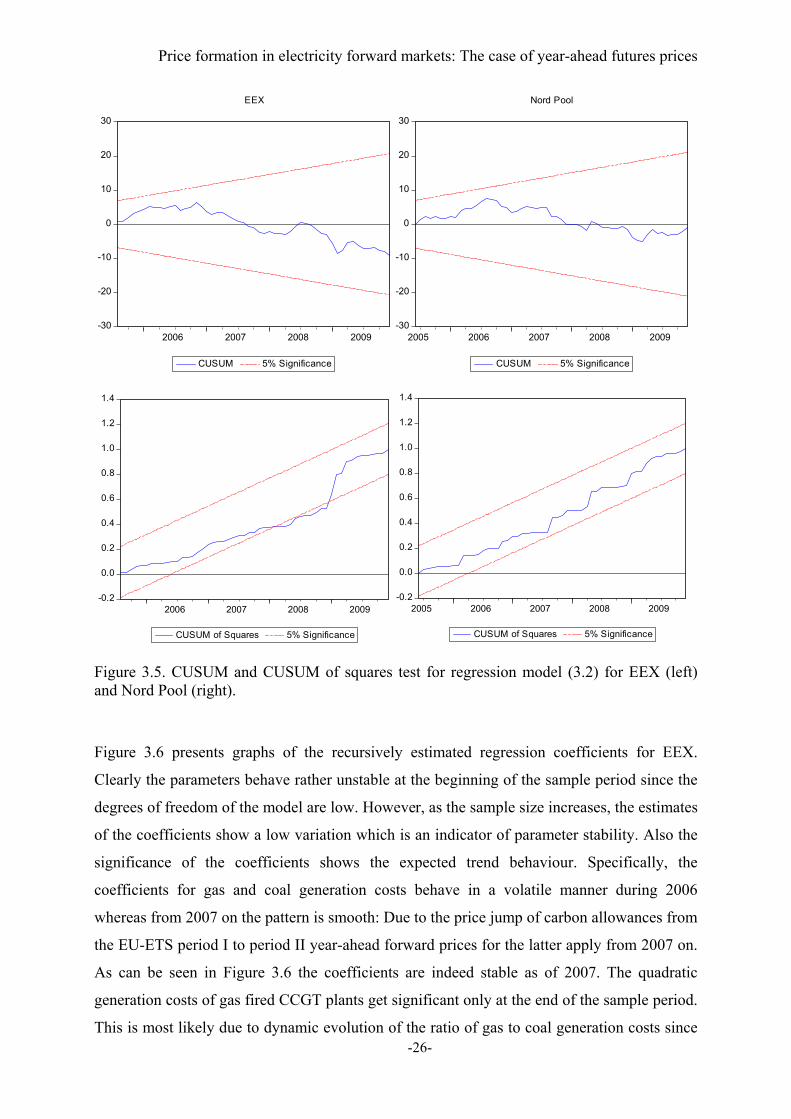
Price formation in electricity forward markets: The case of year-ahead futures prices
-26-
Figure 3.5. CUSUM and CUSUM of squares test for regression model (3.2) for EEX (left) and Nord Pool (right).
Figure 3.6 presents graphs of the recursively estimated regression coefficients for EEX.
Clearly the parameters behave rather unstable at the beginning of the sample period since the
degrees of freedom of the model are low. However, as the sample size increases, the estimates
of the coefficients show a low variation which is an indicator of parameter stability. Also the
significance of the coefficients shows the expected trend behaviour. Specifically, the
coefficients for gas and coal generation costs behave in a volatile manner during 2006
whereas from 2007 on the pattern is smooth: Due to the price jump of carbon allowances from
the EU-ETS period I to period II year-ahead forward prices for the latter apply from 2007 on.
As can be seen in Figure 3.6 the coefficients are indeed stable as of 2007. The quadratic
generation costs of gas fired CCGT plants get significant only at the end of the sample period.
This is most likely due to dynamic evolution of the ratio of gas to coal generation costs since
-30
-20
-10
0
10
20
30
2006 2007 2008 2009
CUSUM 5% Significance
EEX
-30
-20
-10
0
10
20
30
2005 2006 2007 2008 2009
CUSUM 5% Significance
Nord Pool
-0.2
0.0
0.2
0.4
0.6
0.8
1.0
1.2
1.4
2006 2007 2008 2009
CUSUM of Squares 5% Significance
-0.2
0.0
0.2
0.4
0.6
0.8
1.0
1.2
1.4
2005 2006 2007 2008 2009
CUSUM of Squares 5% Significance
Price formation in electricity forward markets: The case of year-ahead futures prices
-27-
more fuel switching towards coal fired plants occurs. Overall, the analysis of recursive
estimates for EEX has confirmed the robustness of the results presented in Table 3.2.
Similarly, Figure 3.7 presents graphs of the recursively estimated regression coefficients for
Nord Pool. As expected the parameters behave rather unstable at the beginning of the sample
period due to the low number of degrees of freedom of the model but, as the sample size
increases, converge quickly as the estimates of the coefficients show a low remaining
variation. This is a clear indicator of parameter stability. Similarly to EEX, the price jump in
the year-ahead carbon market affects the coefficients for gas and coal generation costs
whereas these coefficients behave in stable manner as of 2007. Also all regression coefficients
are statistically significant apart from the first set of observations. Overall, the analysis of
recursive estimates for Nord Pool has confirmed the robustness of the results presented in
Table 3.2. In fact, in terms of parameter stability the Nord Pool model slightly outperforms
the EEX model.
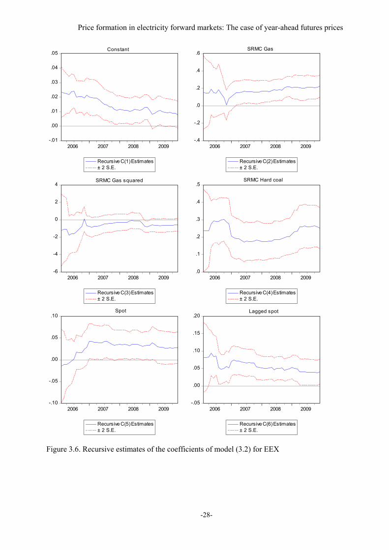
Price formation in electricity forward markets: The case of year-ahead futures prices
-28-
Figure 3.6. Recursive estimates of the coefficients of model (3.2) for EEX
-.01
.00
.01
.02
.03
.04
.05
2006 2007 2008 2009
Recursive C(1) Estimates± 2 S.E.
-.4
-.2
.0
.2
.4
.6
2006 2007 2008 2009
Recursive C(2) Estimates± 2 S.E.
-6
-4
-2
0
2
4
2006 2007 2008 2009
Recursive C(3) Estimates± 2 S.E.
.0
.1
.2
.3
.4
.5
2006 2007 2008 2009
Recursive C(4) Estimates± 2 S.E.
-.10
-.05
.00
.05
.10
2006 2007 2008 2009
Recursive C(5) Estimates± 2 S.E.
-.05
.00
.05
.10
.15
.20
2006 2007 2008 2009
Recursive C(6) Estimates± 2 S.E.
Constant SRMC Gas
SRMC Gas squared SRMC Hard coal
Spot Lagged spot
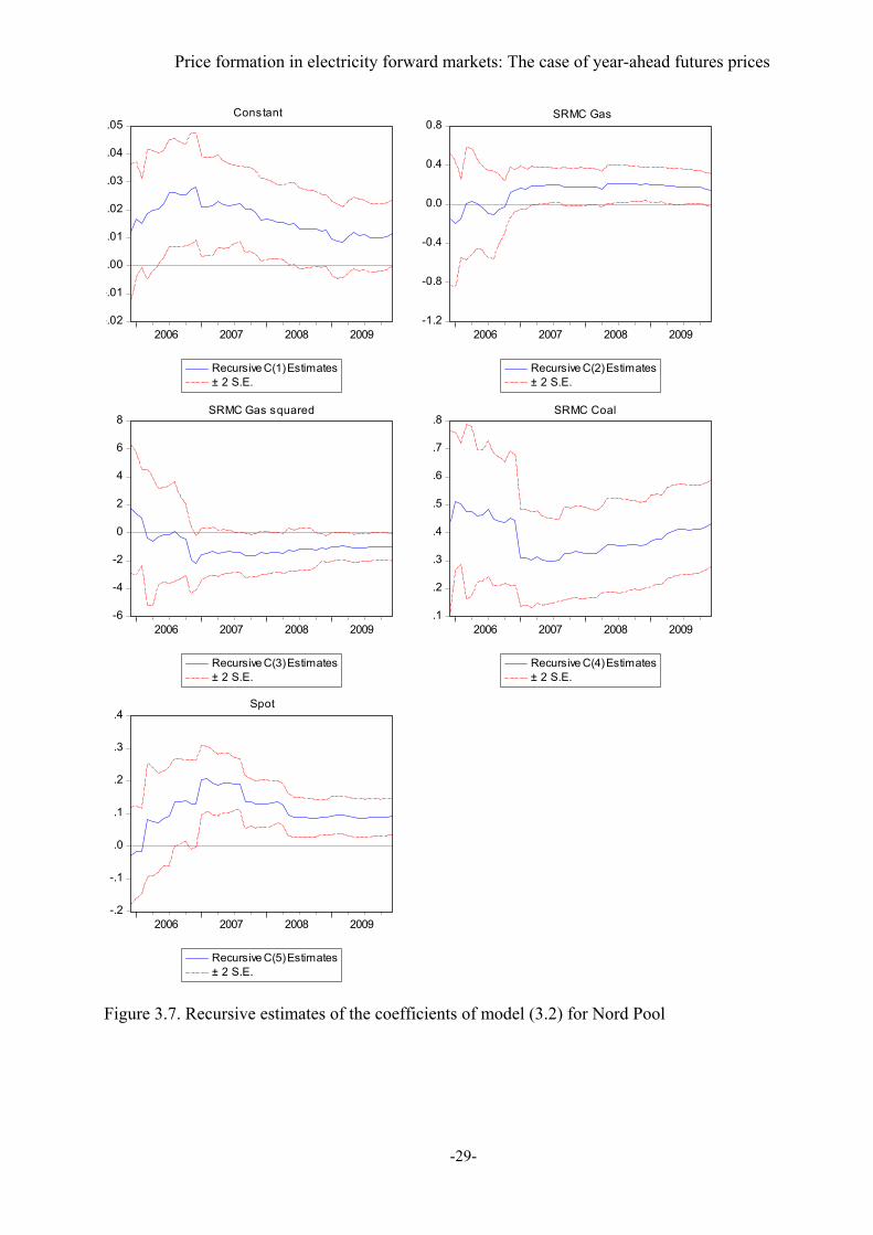
Price formation in electricity forward markets: The case of year-ahead futures prices
-29-
Figure 3.7. Recursive estimates of the coefficients of model (3.2) for Nord Pool
-.02
-.01
.00
.01
.02
.03
.04
.05
2006 2007 2008 2009
Recursive C(1) Estimates± 2 S.E.
-1.2
-0.8
-0.4
0.0
0.4
0.8
2006 2007 2008 2009
Recursive C(2) Estimates± 2 S.E.
-6
-4
-2
0
2
4
6
8
2006 2007 2008 2009
Recursive C(3) Estimates± 2 S.E.
.1
.2
.3
.4
.5
.6
.7
.8
2006 2007 2008 2009
Recursive C(4) Estimates± 2 S.E.
-.2
-.1
.0
.1
.2
.3
.4
2006 2007 2008 2009
Recursive C(5) Estimates± 2 S.E.
Constant SRMC Gas
SRMC Gas squared SRMC Coal
Spot
Price formation in electricity forward markets: The case of year-ahead futures prices
-30-
Interestingly, at both exchanges, the influence of gas and coal fired generation technologies
on electricity prices cannot be distinguished according to a Wald test. The hypothesis of both
power plant types equally influencing forward prices (i.e. b2=b4 in equation (3.2)) cannot be
rejected on a 5% significance level with a χ1DOF-statistic of 0.05 (p-value of 0.82) for EEX
and a χ1DOF-statistic of 3.58 (p-value of 0.06) for Nord Pool. Most likely the introduction of
the EU-ETS contributes to this result yielding a higher competitiveness of gas fired generation
technologies in baseload generation.
With the introduction of the EU-ETS controversial discussions among market participants on
the role of allowance prices and their influence on electricity prices have started. Commonly,
allowance prices were considered as being the prime mover of electricity wholesale prices
although this influence was interpreted as the result of the exercise of market power. Why, it
was argued, would freely allocated emission allowances increase the power price? Still,
simple opportunity cost considerations can resolve this alleged puzzle.
With the empirical model (3.2) it is, however, not possible to assess a potential differing
influence of fuel and CO2 costs on the electricity price directly since splitting up of the fuel
cost and CO2 cost component according to equation (3.1) would lead to multicollinearity
problems when estimating (3.2) by OLS. Instead, to be able to obtain insights regarding the
relative influence of CO2 costs on electricity prices the year-ahead fuel costs and year-ahead
CO2 costs (i.e. the two components of equation (3.1)) are regressed against year-ahead
forward prices separately for CCGT and HC plants:
tTtCCGTTtCCGTTtBase CostLnCObLnFuelCostbbdLnYearAhea ,,23,,21,, (3.3)
tTtHCTtHCTtBase CostLnCObLnFuelCostbbdLnYearAhea ,,23,,21,, (3.4)
where in equation (3.3) ΔLnYearAheadBase,t,T is the growth rate of the year-ahead futures price,
ΔLnFuelCostCCGT,t,T is the growth rate of the fuel cost component of the year-ahead generation
costs of gas fired power plants and ΔLnCO2CostCCGT,t,T is the growth rate of the CO2 cost
component of year-ahead generation costs of gas fired power plants. Similarly, equation (3.4)
estimates the year-ahead futures price on the fuel and CO2 cost components of coal fired
power plants. Table 3.3 shows the detailed results of the econometric models for the EEX and
Nord Pool markets.
According to the model results both fuel costs and CO2 costs significantly influence forward
prices at the EEX and the Nord Pool. This, clearly, is to be expected. As CO2 emissions from
energy activities are part of the EU-ETS, market prices of emission allowances represent

Price formation in electricity forward markets: The case of year-ahead futures prices
-31-
opportunity costs which affect electricity generation costs of fossil fuelled power plants.
Hence, given CO2 emitting price setting technologies, CO2 costs are part of electricity
wholesale prices. This result applies irrespective of the allocation mechanism of CO2 emission
allowances.
Table 3.3. Results of regression analysis (3.3) and (3.4) for Δ Ln Year-ahead base load futures traded during December 2004 to December 2009 at the EEX and Nord Pool exchanges (t-statistics in brackets). All tests are based on heteroscedasticity consistent standard errors. *, **, *** denotes significance on the 10%, 5% and 1%-level.
Coefficient Variable EEX Nord Pool
CCGT HC CCGT HC
b1 Constant term 0.001 (1.16) 0.003 (0.72) 0.01 (0.86) 0.003 (0.63)
b2 Δ Ln Fuel cost t,T 0.35 (6.03)*** 0.40 (6.94)*** 0.36 (4.33)*** 0.52 (7.27)***
b3 Δ Ln CO2 cost t,T 0.10 (2.24)** 0.13 (2.96)*** 0.17 (2.79)*** 0.19 (3.11)***
R2 (R2corr) 0.64 (0.63) 0.62 (0.61) 0.57 (0.56) 0.66 (0.65)
DW 1.30 1.24 1.36 1.19
Serial correlation χ212DOF (p-value) 0.181 0.228 0.116 0.0043
Functional form χ21DOF (p-value) 0.02 0.007 0 0.001
Normality χ22DOF (p-value) 0.817 0.404 0.774 0.13
Heteroscedasticity χ22DOF (p-value) 0.487 0.67 0.035 0.04
Observations 60 60 60 60
3.3 Conclusions
Due to lacking storage possibilities, no exact relationship between current spot and forward
prices can be formulated. Instead, forward prices are built on expectations of market
participants, updated by applying forward premia. The analysis on year-ahead electricity
prices in this chapter has revealed three corresponding results concerning the expectation
formation worth emphasising.
First, year-ahead baseload electricity prices do depend on year-ahead generation costs in line
with economic theory on equilibrium relationships for forward pricing. The year-ahead
generation costs can be interpreted as the market’s best estimate of future electricity prices.
Second, electricity forward prices are also influenced by current spot prices. Moreover, the
recent trend of spot prices has a significant impact on the futures price.
This suggests the existence of a behavioural pricing component in the forward market.
Trading strategies of market participants seem to rely partly on current spot prices instead of
fundamental modelling approaches. Finally, although the EEX and Nord Pool market are
physically only weakly interconnected – resulting in different price levels – main

Price formation in electricity forward markets: The case of year-ahead futures prices
-32-
characteristics with regard to price formation on the year-ahead forward markets are alike
although the supply and demand side characteristics in the EEX market differ significantly
from the fundamentals in the Nord Pool market.
Clearly, the significant influence of current spot market prices on futures prices in both
markets questions the forecasting power of the forward price (i.e. the consistency of the
forward price). Hence, it is of interest to study the relationship between current spot and
forward prices and market participants’ corresponding risk assessment in more detail. The
next chapter will specifically assess the interaction of spots and forwards. Chapter 5 will, in
turn, study the implications for the price of risk inherent in forward price quotations.
Interaction between spot and forward prices
-33-
4 Interaction between spot and forward prices
Assuming rational expectations and risk-neutral market actors, future spot prices should only
deviate from forward prices in case of unexpected shocks. Therefore, under these stringent
assumptions, spot prices in the delivery period ST should equal forward prices Ft,T plus a white
noise error term εt with zero mean:
tTtTtTtTt FSSEF ,, )( (4.1)
The results of the empirical models presented in Chapter 3 question the predictive power of
the year-ahead forward price however as it depends on current spot prices. Therefore, this
chapter will explore this relationship more closely. A traditional approach to test hypothesis
(4.1) is to run a regression where the spot price is regressed against a constant and the futures
price. If the forward price were an unbiased predictor of the future spot price the regression
coefficients of the constant term and the futures price should not be statistically different from
zero and one respectively.
Price time series often exhibit a non-stationary behaviour. To avoid spurious regression
results differences of the time series have to be considered which, however, eliminates
important long run information. Nevertheless, if the time series are cointegrated OLS
estimation can be used without taking differences of the relevant time series (Engle and
Granger, 1987).
This structural approach necessitates a clear distinction between exogenous and endogenous
variables. However, the distinction might not be clear cut in the case of spot and forward
markets. Clearing on these markets is a result of market forces and their interactions which
precludes that one development on one market is fixed and determines the development on
the other market. Instead, a simultaneous evolution may be assumed. Furthermore, Gjolberg
and Brattested (2011) point out additional econometric and fundamental problems associated
with tests of equations similar to (4.1).
Interestingly, for electricity spot and forward markets the distinction is not as clear cut as
commonly recognised. A link between current spot and current forward prices might not be
anticipated due to the fact that electricity is not storable. Finding a corresponding relationship
may, accordingly, suggest a behavioural pricing component prevailing in the markets.
Fundamentally, power prices are affected by production costs, demand, and market power
(Bunn, 2004, Weron, 2006). The inputs to electricity production (gas, coal and CO2 permits)
Interaction between spot and forward prices
-34-
are, however, storable.40 Hence, links between electricity spots and forwards can emerge from
the fact that electricity is a derived commodity.41 This necessitates a careful variable selection
for an empirical analysis of prices (and corresponding links).
The relations between electricity spots and forwards may not only emerge from links in
storable fuels. Also, counter to the implications of rational pricing models, behavioural biases
(e.g. caused by employing heuristics or anchoring decisions) are reasonably to be expected to
prevail in electricity markets.42
Interestingly, despite rich literature on explicit stochastic spot and forward price models and
empirical analyses of the properties of risk premia, few studies specifically dealt with (high-
frequency and short-term) interactions of electricity spot and futures prices. Bunn and
Gianfreda (2009) estimate the integration of different regional European spot and futures
electricity markets using Granger, cointegration and impulse response tests and find
significant interactions among European spot markets and also among European futures
markets. Similarly, Bunn and Fezzi (2008) and Fell (2010) study in detail the interactions
between carbon, fuel and electricity spot prices. However, the above studies do not assess
interactions between electricity spots and forwards in the same regional market. I specifically
seek to address this issue in the following. Shawky et al. (2003) constitutes a first exception
for electricity. They estimate an EGARCH and a VAR model and find that conditional
volatility and shocks to spot returns determine the relation between spots and forwards. Most
of the empirical literature available on price interactions studies, obviously, oil prices. Ng and
Pirrong (1996) provide an early analysis for petroleum products using non-linear error
correction models and find (current) futures prices leading (current) spot prices. Newer work
on oil includes Kaufmann and Ullman (2009) and Bekiros and Diks (2008).43 Depending on
the sample and applied methodology results differ – generally, they suggest mixed lead/lag
relation between spots and forwards. Finally, Gronwald et al. (2010) apply Granger causality
tests on European CO2 spot and futures prices finding a bi-directional relationship.
Figure 4.1 depicts the evolution of daily EEX spot and forward (month-ahead, quarter-ahead
and year-ahead) prices. Generally, stable market periods can be distinguished from trending
40 Chapter 3 has shown that fossil fuelled power plants are price setting in the EEX market. 41 Douglas and Popova (2008) show that gas inventory levels can affect electricity day-ahead forward premia by influencing the moments of electricity prices. This chapter aims to analyse the effect of storable fuels on the futures prices themselves. 42 See Chapter 5 for a detailed analysis. 43 See also the references therein.
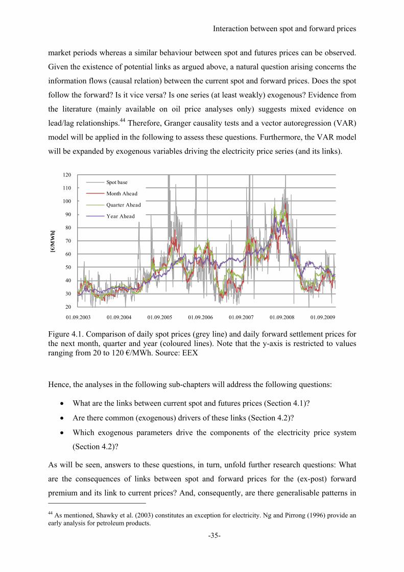
Interaction between spot and forward prices
-35-
market periods whereas a similar behaviour between spot and futures prices can be observed.
Given the existence of potential links as argued above, a natural question arising concerns the
information flows (causal relation) between the current spot and forward prices. Does the spot
follow the forward? Is it vice versa? Is one series (at least weakly) exogenous? Evidence from
the literature (mainly available on oil price analyses only) suggests mixed evidence on
lead/lag relationships.44 Therefore, Granger causality tests and a vector autoregression (VAR)
model will be applied in the following to assess these questions. Furthermore, the VAR model
will be expanded by exogenous variables driving the electricity price series (and its links).
Figure 4.1. Comparison of daily spot prices (grey line) and daily forward settlement prices for the next month, quarter and year (coloured lines). Note that the y-axis is restricted to values ranging from 20 to 120 €/MWh. Source: EEX
Hence, the analyses in the following sub-chapters will address the following questions:
What are the links between current spot and futures prices (Section 4.1)?
Are there common (exogenous) drivers of these links (Section 4.2)?
Which exogenous parameters drive the components of the electricity price system
(Section 4.2)?
As will be seen, answers to these questions, in turn, unfold further research questions: What
are the consequences of links between spot and forward prices for the (ex-post) forward
premium and its link to current prices? And, consequently, are there generalisable patterns in 44 As mentioned, Shawky et al. (2003) constitutes an exception for electricity. Ng and Pirrong (1996) provide an early analysis for petroleum products.
20
30
40
50
60
70
80
90
100
110
120
01.09.2003 01.09.2004 01.09.2005 01.09.2006 01.09.2007 01.09.2008 01.09.2009
[€/M
Wh]
Spot base
Month Ahead
Quarter Ahead
Year Ahead
Interaction between spot and forward prices
-36-
the forward premium evolution as a function of time to maturity? These questions will be
assessed in detail in Chapter 5 and Appendix B.
Several issues have to be considered before judging too quickly on generalisable patterns in
the links between spots and forwards. Trading is thin for contracts with maturities more
distant in the future. Hence, a model representation including all currently traded products
may not touch upon the relevant relations which were governed by actual trading and
corresponding “fundamental” market liquidities. A related fact concerns that due to arbitrage
prices of several contracts can be determined by the other products on the market which
brings about problems of endogeneity. For prices observed in January, for example, the price
of the second quarter contract must be the average of the prices for monthly futures for April,
May and June updated by transaction cost. Hence, in order to avoid these problems the
analysis presented below focuses on spot and one month-, quarter-, and year-ahead prices (see
Figure 4.1).
4.1 The link between current spot and futures prices
The finally to be employed empirical methodology depends on the properties of the analysed
daily price time series. All time series depicted in Figure 4.1 are non-normally distributed and
are highly correlated with correlation coefficients exceeding a minimum value of 0.58
(between current year-ahead and spot prices) and ranging up to 0.92 (between month and
quarter-ahead prices).45 Table 4.1 summarises the correlation coefficients and shows
descriptive statistics of the individual distributions. To filter out the relationship only working
days are used for the price time series since futures contracts are not traded on weekends and
public holidays.
All time series except the spot prices contain a unit root. Hence, an analysis in levels could be
performed for the forwards only if the respective time series were cointegrated.46 Since the
analysis comprises stationary spot prices an unrestricted VAR model is tested for the returns
(i.e. the logarithmic differences) of the original price series instead. This transformation has to
be kept in mind when interpreting the model results. As shown in Figure 4.2 the return series
are clearly stationary (which is confirmed by unit root tests). Table 4.2 summarises the
correlation coefficients and shows descriptive statistics of the returns data set.
45 These correlations may appear surprisingly high given a non-storable commodity. 46 The futures price series are non-stationary when including an intercept as well as a linear trend in the test equation.
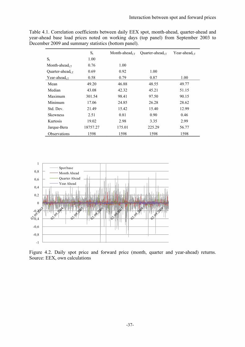
Interaction between spot and forward prices
-37-
Table 4.1. Correlation coefficients between daily EEX spot, month-ahead, quarter-ahead and year-ahead base load prices noted on working days (top panel) from September 2003 to December 2009 and summary statistics (bottom panel).
St Month-aheadt,T Quarter-aheadt,T Year-aheadt,T
St 1.00
Month-aheadt,T 0.76 1.00
Quarter-aheadt,T 0.69 0.92 1.00
Year-aheadt,T 0.58 0.79 0.87 1.00
Mean 49.20 46.88 48.55 49.77
Median 43.08 42.32 45.21 51.15
Maximum 301.54 98.41 97.50 90.15
Minimum 17.06 24.85 26.28 28.62
Std. Dev. 21.49 15.42 15.40 12.99
Skewness 2.51 0.81 0.90 0.46
Kurtosis 19.02 2.98 3.35 2.99
Jarque-Bera 18757.27 175.01 225.29 56.77
Observations 1598 1598 1598 1598
Figure 4.2. Daily spot price and forward price (month, quarter and year-ahead) returns. Source: EEX, own calculations
-1
-0,8
-0,6
-0,4
-0,2
0
0,2
0,4
0,6
0,8
1Spot base
Month Ahead
Quarter Ahead
Year Ahead

Interaction between spot and forward prices
-38-
Table 4.2. Correlation coefficients between daily EEX spot and futures returns (top panel) from September 2003 to December 2009 and summary statistics (bottom panel).
St ΔLogMonthAheadt,T ΔLogQuarterAheadt,T ΔLogYearAheadt,T
ΔLogSt 1.00
ΔLogMonthAheadt,T -0.031 1.00
ΔLogQuarterAheadt,T -0.003 0.339 1.00
ΔLogYearAheadt,T -0.059 0.386 0.438 1.00
Mean 0.000 0.000 0.000 0.000
Median 0.003 -0.001 0.000 0.000
Maximum 1.096 0.276 0.328 0.102
Minimum -1.076 -0.150 -0.304 -0.087
Std. Dev. 0.178 0.032 0.026 0.012
Skewness -0.096 1.953 1.291 -0.008
Kurtosis 8.733 18.747 67.311 11.988
Jarque-Bera 2189.145 17515.330 275653.900 5375.611
Observations 1597 1597 1597 1597
To assess the interrelation between spot and forward prices an unrestricted vector
autoregression (VAR) model is estimated:
tptpttt yAyAyAAy ...22110 (4.2)
where
)(
)()(
)(
1,
1,
1,
1,
Ytt
Qtt
Mtt
tt
t
FLog
FLogFLog
SLog
y is a vector of spot and forward price returns, A0 is a vector of
constants, and A1, etc. are the coefficient matrices. ΔLog(St,t+1) is the daily return in the day-
ahead spot market, ΔLog(Ft,t+1M), ΔLog(Ft,t+1Q), and ΔLog(Ft,t+1Y) are the month-, quarter-, and
year-ahead futures price returns. Lag length criteria suggest a lag length of 1 (SC), 2 (HQ) and
5 (AIC). Since lag exclusion tests yield significant lags up to the second one, a lag length of
two is selected. However, significant autocorrelation is still prevalent in the residuals (most
likely due to omitted exogenous variables). Table 4.3 shows the results of the VAR model.
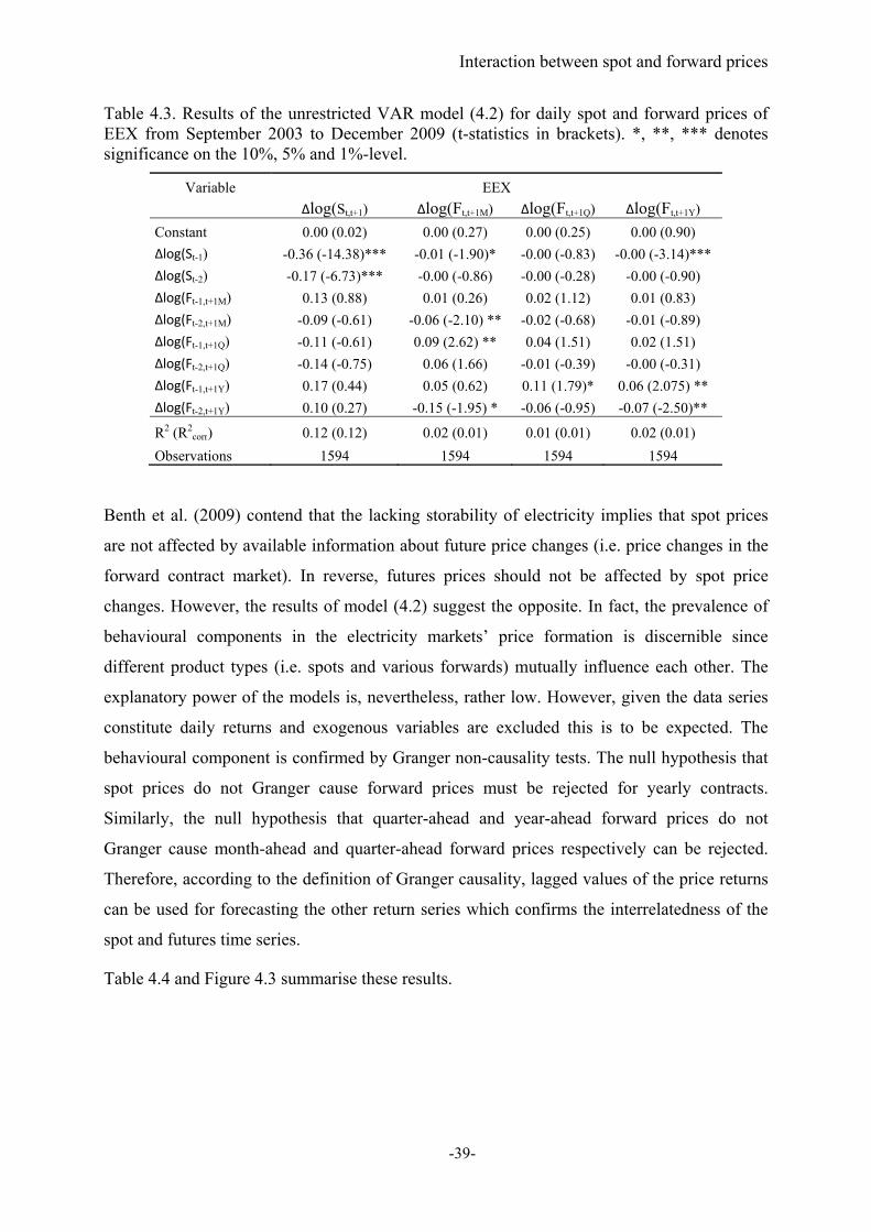
Interaction between spot and forward prices
-39-
Table 4.3. Results of the unrestricted VAR model (4.2) for daily spot and forward prices of EEX from September 2003 to December 2009 (t-statistics in brackets). *, **, *** denotes significance on the 10%, 5% and 1%-level.
Variable EEX
Δlog(St,t+1) Δlog(Ft,t+1M) Δlog(Ft,t+1Q) Δlog(Ft,t+1Y)
Constant 0.00 (0.02) 0.00 (0.27) 0.00 (0.25) 0.00 (0.90)
Δlog(St-1) -0.36 (-14.38)*** -0.01 (-1.90)* -0.00 (-0.83) -0.00 (-3.14)***
Δlog(St-2) -0.17 (-6.73)*** -0.00 (-0.86) -0.00 (-0.28) -0.00 (-0.90)
Δlog(Ft-1,t+1M) 0.13 (0.88) 0.01 (0.26) 0.02 (1.12) 0.01 (0.83)
Δlog(Ft-2,t+1M) -0.09 (-0.61) -0.06 (-2.10) ** -0.02 (-0.68) -0.01 (-0.89)
Δlog(Ft-1,t+1Q) -0.11 (-0.61) 0.09 (2.62) ** 0.04 (1.51) 0.02 (1.51)
Δlog(Ft-2,t+1Q) -0.14 (-0.75) 0.06 (1.66) -0.01 (-0.39) -0.00 (-0.31)
Δlog(Ft-1,t+1Y) 0.17 (0.44) 0.05 (0.62) 0.11 (1.79)* 0.06 (2.075) **
Δlog(Ft-2,t+1Y) 0.10 (0.27) -0.15 (-1.95) * -0.06 (-0.95) -0.07 (-2.50)**
R2 (R2corr) 0.12 (0.12) 0.02 (0.01) 0.01 (0.01) 0.02 (0.01)
Observations 1594 1594 1594 1594
Benth et al. (2009) contend that the lacking storability of electricity implies that spot prices
are not affected by available information about future price changes (i.e. price changes in the
forward contract market). In reverse, futures prices should not be affected by spot price
changes. However, the results of model (4.2) suggest the opposite. In fact, the prevalence of
behavioural components in the electricity markets’ price formation is discernible since
different product types (i.e. spots and various forwards) mutually influence each other. The
explanatory power of the models is, nevertheless, rather low. However, given the data series
constitute daily returns and exogenous variables are excluded this is to be expected. The
behavioural component is confirmed by Granger non-causality tests. The null hypothesis that
spot prices do not Granger cause forward prices must be rejected for yearly contracts.
Similarly, the null hypothesis that quarter-ahead and year-ahead forward prices do not
Granger cause month-ahead and quarter-ahead forward prices respectively can be rejected.
Therefore, according to the definition of Granger causality, lagged values of the price returns
can be used for forecasting the other return series which confirms the interrelatedness of the
spot and futures time series.
Table 4.4 and Figure 4.3 summarise these results.
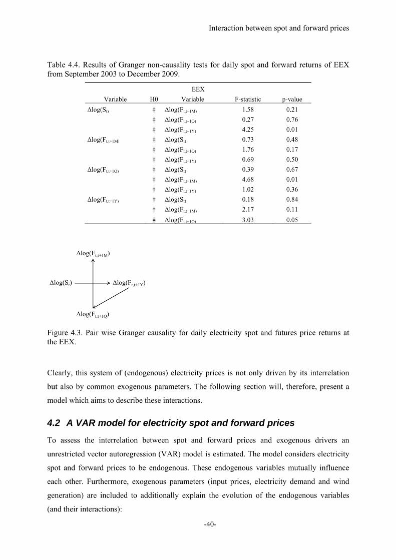
Interaction between spot and forward prices
-40-
Table 4.4. Results of Granger non-causality tests for daily spot and forward returns of EEX from September 2003 to December 2009.
EEX
Variable H0 Variable F-statistic p-value
Δlog(St) ǂ Δlog(Ft,t+1M) 1.58 0.21
ǂ Δlog(Ft,t+1Q) 0.27 0.76
ǂ Δlog(Ft,t+1Y) 4.25 0.01
Δlog(Ft,t+1M) ǂ Δlog(St) 0.73 0.48
ǂ Δlog(Ft,t+1Q) 1.76 0.17
ǂ Δlog(Ft,t+1Y) 0.69 0.50
Δlog(Ft,t+1Q) ǂ Δlog(St) 0.39 0.67
ǂ Δlog(Ft,t+1M) 4.68 0.01
ǂ Δlog(Ft,t+1Y) 1.02 0.36
Δlog(Ft,t+1Y) ǂ Δlog(St) 0.18 0.84
ǂ Δlog(Ft,t+1M) 2.17 0.11
ǂ Δlog(Ft,t+1Q) 3.03 0.05
Figure 4.3. Pair wise Granger causality for daily electricity spot and futures price returns at the EEX.
Clearly, this system of (endogenous) electricity prices is not only driven by its interrelation
but also by common exogenous parameters. The following section will, therefore, present a
model which aims to describe these interactions.
4.2 A VAR model for electricity spot and forward prices
To assess the interrelation between spot and forward prices and exogenous drivers an
unrestricted vector autoregression (VAR) model is estimated. The model considers electricity
spot and forward prices to be endogenous. These endogenous variables mutually influence
each other. Furthermore, exogenous parameters (input prices, electricity demand and wind
generation) are included to additionally explain the evolution of the endogenous variables
(and their interactions):
Δlog(St) Δlog(Ft,t+1Y)
Δlog(Ft,t+1M)
Δlog(Ft,t+1Q)
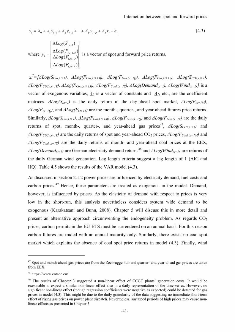
Interaction between spot and forward prices
-41-
ttxptpttt xAyAyAyAAy ...22110 (4.3)
where
)(
)()(
)(
1,
1,
1,
1,
Ytt
Qtt
Mtt
tt
t
FLog
FLogFLog
SLog
y is a vector of spot and forward price returns,
xtT=[ΔLog(SGas,t,t+1), ΔLog(FGas,t,t+1M), ΔLog(FGas,t,t+1Q), ΔLog(FGas,t,t+1Y), ΔLog(SCO2,t,t+1),
ΔLog(FCO2,t,t+1Y), ΔLog(FCoal,t,t+1M), ΔLog(FCoal,t,t+1Y), ΔLog(Demandt,t+1), ΔLog(Windt,t+1)] is a
vector of exogenous variables, A0 is a vector of constants and A1, etc., are the coefficient
matrices. ΔLog(St,t+1) is the daily return in the day-ahead spot market, ΔLog(Ft,t+1M),
ΔLog(Ft,t+1Q), and ΔLog(Ft,t+1Y) are the month-, quarter-, and year-ahead futures price returns.
Similarly, ΔLog(SGas,t,t+1), ΔLog(FGas,t,t+1M), ΔLog(FGas,t,t+1Q) and ΔLog(FGas,t,t+1Y) are the daily
returns of spot, month-, quarter-, and year-ahead gas prices47, ΔLog(SCO2,t,t+1) and
ΔLog(FCO2,t,t+1Y) are the daily returns of spot and year-ahead CO2 prices, ΔLog(FCoal,t,t+1M) and
ΔLog(FCoal,t,t+1Y) are the daily returns of month- and year-ahead coal prices at the EEX,
ΔLog(Demandt,t+1) are German electricity demand returns48 and ΔLog(Windt,t+1) are returns of
the daily German wind generation. Lag length criteria suggest a lag length of 1 (AIC and
HQ). Table 4.5 shows the results of the VAR model (4.3).
As discussed in section 2.1.2 power prices are influenced by electricity demand, fuel costs and
carbon prices.49 Hence, these parameters are treated as exogenous in the model. Demand,
however, is influenced by prices. As the elasticity of demand with respect to prices is very
low in the short-run, this analysis nevertheless considers system wide demand to be
exogenous (Karakatsani and Bunn, 2008). Chapter 5 will discuss this in more detail and
present an alternative approach circumventing the endogeneity problem. As regards CO2
prices, carbon permits in the EU-ETS must be surrendered on an annual basis. For this reason
carbon futures are traded with an annual maturity only. Similarly, there exists no coal spot
market which explains the absence of coal spot price returns in model (4.3). Finally, wind
47 Spot and month-ahead gas prices are from the Zeebrugge hub and quarter- and year-ahead gas prices are taken from EEX. 48 https://www.entsoe.eu/ 49 The results of Chapter 3 suggested a non-linear effect of CCGT plants’ generation costs. It would be reasonable to expect a similar non-linear effect also in a daily representation of the time-series. However, no significant non-linear effect (though regression coefficients were negative as expected) could be detected for gas prices in model (4.3). This might be due to the daily granularity of the data suggesting no immediate short-term effect of rising gas prices on power plant dispatch. Nevertheless, sustained periods of high prices may cause non-linear effects as presented in Chapter 3.
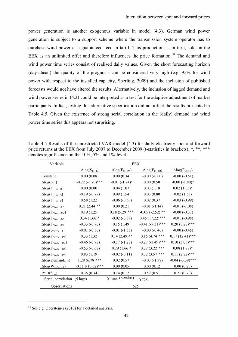
Interaction between spot and forward prices
-42-
power generation is another exogenous variable in model (4.3). German wind power
generation is subject to a support scheme where the transmission system operator has to
purchase wind power at a guaranteed feed in tariff. This production is, in turn, sold on the
EEX as an unlimited offer and therefore influences the price formation.50 The demand and
wind power time series consist of realised daily values. Given the short forecasting horizon
(day-ahead) the quality of the prognosis can be considered very high (e.g. 95% for wind
power with respect to the installed capacity, Sperling, 2009) and the inclusion of published
forecasts would not have altered the results. Alternatively, the inclusion of lagged demand and
wind power series in (4.3) could be interpreted as a test for the adaptive adjustment of market
participants. In fact, testing this alternative specification did not affect the results presented in
Table 4.5. Given the existence of strong serial correlation in the (daily) demand and wind
power time series this appears not surprising.
Table 4.5 Results of the unrestricted VAR model (4.3) for daily electricity spot and forward price returns at the EEX from July 2007 to December 2009 (t-statistics in brackets). *, **, *** denotes significance on the 10%, 5% and 1%-level.
Variable EEX
Δlog(St,t+1) Δlog(Ft,t+1M) Δlog(Ft,t+1Q) Δlog(Ft,t+1Y)
Constant 0.00 (0.08) 0.00 (0.34) -0.00 (-0.00) -0.00 (-0.51)
Δlog(St-1) -0.22 (-6.70)*** -0.01 (-1.74)* 0.00 (0.50) -0.00 (-1.80)*
Δlog(Ft-1,t+1M) 0.00 (0.00) 0.04 (1.07) 0.03 (1.18) 0.02 (1.65)*
Δlog(Ft-1,t+1Q) -0.19 (-0.77) 0.09 (1.54) 0.03 (0.80) 0.02 (1.33)
Δlog(Ft-1,t+1Y) 0.58 (1.22) -0.06 (-0.56) 0.02 (0.37) -0.03 (-0.99)
Δlog(SGas,t,t+1) 0.21 (2.44)** 0.00 (0.21) -0.01 (-1.14) -0.01 (-1.08)
Δlog(FGas,t,t+1M) 0.19 (1.25) 0.18 (5.29)*** -0.05 (-2.52) ** -0.00 (-0.37)
Δlog(FGas,t,t+1Q) 0.34 (1.66)* -0.02 (-0.39) 0.45 (17.22)*** -0.01 (-0.98)
Δlog(FGas,t,t+1Y) -0.33 (-0.76) 0.15 (1.49) -0.41 (-7.31)*** 0.20 (8.28)***
Δlog(SCO2,t,t+1) -0.01 (-0.56) -0.01 (-1.35) -0.00 (-0.46) -0.00 (-0.45)
Δlog(FCO2,t,t+1Y) 0.33 (1.32) 0.14 (2.49)** 0.15 (4.74)*** 0.17 (12.41)***
Δlog(FCoal,t,t+1M) -0.46 (-0.78) -0.17 (-1.28) -0.27 (-3.49)*** 0.10 (3.05)***
Δlog(FCoal,t,t+1Q) -0.53 (-0.68) 0.29 (1.66)* 0.32 (3.22)*** 0.08 (1.88)*
Δlog(FCoal,t,t+1Y) 0.83 (1.19) -0.02 (-0.11) 0.32 (3.57)*** 0.11 (2.82)***
Δlog(Demandt,t+1) 1.28 (6.78)*** 0.02 (0.57) -0.03 (-1.38) -0.04 (-3.39)***
Δlog(Windt,t+1) -0.11 (-16.02)*** 0.00 (0.05) 0.00 (0.12) 0.00 (0.25)
R2 (R2corr) 0.35 (0.34) 0.14 (0.12) 0.52 (0.51) 0.71 (0.70)
Serial correlation (5 lags) χ216DOF (p-value) 0.725
Observations 625
50 See e.g. Obersteiner (2010) for a detailed analysis.
Interaction between spot and forward prices
-43-
Electricity spot price returns are significantly negatively influenced by its lagged value which
is consistent with mean reversion properties of the stationary spot price series. As expected
gas spot price returns (significantly) positively influence electricity spot returns. However,
also returns of quarterly gas futures influence electricity spot returns on a 10% significance
level. This result might be a consequence of the cost of carry in the storable fuel gas. The
fundamental supply and demand variables significantly influence the spot price returns and
show the expected signs (i.e. positive for demand and negative for wind power). Interestingly,
carbon spot price returns do not affect electricity returns. This seems puzzling. As discussed
in Chapter 3 CO2 certificate prices represent opportunity costs and are therefore part of
electricity prices. Moreover, the analysis in section 3.2 has shown that year-ahead futures
prices are significantly influenced by carbon returns. Similarly, the results of the fundamental
marginal cost model for EEX spot prices presented in section 5.5 (see Figure 5.7) indicate a
full pass through of CO2 allowance prices on a monthly basis. Still, the results of model (4.3)
suggest that on a high(er) frequency basis (i.e. daily) carbon spot price returns do not affect
the electricity price return system. There is, however, an explanation for this result. Electricity
spot returns are positively influenced by carbon futures returns on a (weak) 15% significance
level. Apart from the year 2007 (i.e. the last year of the first period of the EU-ETS) carbon
spot and futures prices are highly correlated due to the storability of carbon permits.51 Hence,
carbon year-ahead futures returns capture the CO2-related movement of the electricity price
return system for all maturities of the latter (from spot to year-ahead) as will be seen in the
following.52
Returns of month-ahead futures are negatively influenced by spot price returns on a 10% level
whereas lagged values of month-ahead returns do not influence the former. As expected gas
month-ahead price returns (significantly) positively influence electricity month-ahead returns.
Year-ahead carbon returns do positively affect the month-ahead electricity returns which, at
first sight, appears counterintuitive but can be explained by the fact that CO2 allowances must
be surrendered annually and, moreover, the storability of carbon permits implies a strong link
between year-ahead prices and those of spot prices (and “virtual” maturities in between). Coal
month-ahead futures returns do, interestingly, not influence the corresponding electricity
returns whereas coal quarter-ahead returns do. Similar to CO2, this can be explained by the
51 Including a dummy variable for the first trading period of the EU-ETS did not alter the results presented in Table 4.5. 52 Bunn and Fezzi (2008) show that UK and German spot electricity prices are not affected by carbon spot prices. However, they do not consider carbon futures in their model.
Interaction between spot and forward prices
-44-
storability of coal which implies a high correlation of coal month- and quarter-ahead futures
prices.
Returns of quarter-ahead electricity futures are not influenced by the electricity return system
which seems to contradict the results of the Granger non-causality tests presented in Table 4.4
indicating Granger causality running from year-ahead to quarter-ahead returns. However,
model (4.3) has to rely on a shorter sample size and the movement of the endogenous
variables in this model is largely driven by exogenous variables. Gas quarter-ahead price
returns (significantly) positively influence electricity quarter-ahead returns whereas there is
also a negative effect of gas month- and year-ahead returns.
Returns of year-ahead electricity futures are influenced by electricity spot returns (in
accordance with the Granger non-causality tests presented in Table 4.4 indicating Granger
causality running from spot to year-ahead returns and the results presented in chapter 3) and
month-ahead returns. Gas, coal and carbon year-ahead price returns (significantly) positively
influence electricity year-ahead returns which is to be expected whereas returns of coal
month- and quarter-ahead futures also positively influence year-ahead electricity returns.
There might be an interaction affect between the coal futures returns causing this result.
Reinforcing the interpretation of behavioural pricing components, a small negative (but
significant) affect of the day-ahead demand returns on the year-ahead electricity futures return
can be detected.53
In general, a link between electricity spot and futures prices may not only emerge from a
behavioural bias. Given storable fuels as production inputs (coal, gas and CO2 permits) a link
in electricity may possibly follow from the cost of carry in those inputs. Still, both exogenous
variables and endogenous electricity (spot) prices are significant in (4.3). Moreover, the
correlation between inputs and spots in (4.3) is low ruling out multicollinearity concerns. This
indicates an important influence of the spot price on the futures price itself.54
53 In terms of behavioural pricing components Chapter 5 will argue that oil market volatility spills over to the price of risk in electricity markets. Accordingly, it might be reasonable to expect a similar effect when assessing the price formation itself. Still, regression coefficients for oil prices turned out insignificant when included in model (4.3). This reinforces the interpretation presented in Chapter 5 that oil markets are relevant for the risk assessment of electricity wholesale market participants. 54 Performed regressions on the electricity basis (the difference between current futures and spot prices) on the basis prevailing in the gas, coal and CO2 markets indeed yielded significant effects. This result implies the spill over of the cost of carry of input fuels to the non-storable commodity electricity. Nevertheless, these regressions also yielded significant influences of lags of the electricity basis (In fact, the regressions are misspecified if only the carrying costs are included). This, again, indicates a behavioural bias. Results are available upon request.

Interaction between spot and forward prices
-45-
4.3 Conclusions
The analysis in this chapter has disclosed several interesting results. Firstly, Granger-non
causality tests have revealed significant interactions among spot price returns and month-,
quarter-, and year-ahead futures price returns casting doubt on a clear distinction between
short and long term markets. This suggests the existence of behavioural pricing components
and rejects claims on a supposedly exogeneity – caused by the non-storability of electricity –
of spot prices on the one hand and forward prices on the other.
Secondly, these results are confirmed by VAR regression models. Although the modelled
time series are returns (i.e. logarithmic differences) the coefficient of determination R2 is
satisfactorily high (up to 70% for year-ahead returns) in the above presented models. More
specifically, the movement of the electricity price system can, to a large extent, be explained
by exogenous supply and demand side variables driving the electricity prices. Still, there are
strong interactions between the electricity price series confirmed by significant regression
coefficients in the VAR models (which accords with Granger non-causality tests).
The results of the regression models additionally suggest the prevalence of behavioural
pricing components in the markets which, in turn, casts doubts on the predictive power of
forward prices and, in turn, on market efficiency. Additionally, the tie in storable fuels implies
the corresponding cost of carry also effecting the non-storable commodity electricity. This
complicates the price formation. The risk assessment of market participants might be affected
increasing the cost of hedging spot price uncertainty.
What are the implications of this potentially lacking informational function of the forwards?
What are the drivers of the corresponding bias? How is the risk assessment of market
participants affected? The next chapter will analyse these questions in detail.
Components of the forward market premium in electricity
-46-
5 Components of the forward market premium in
electricity 55
This chapter presents a multifactor empirical analysis of the determinants of the realised
premia in forward prices for electricity, when compared to their associated spot prices.
Considering a wide-ranging set of factors involving fundamental, behavioural, dynamic,
market conduct and shock components, a number of propositions are tested on a long data set
from the most liquid of European forward markets, the EEX. It is shown that parts of what is
conventionally regarded as the market price of risk in electricity is actually that of its
underlying fuel commodity, gas; that market power has a double effect on prices,
notwithstanding the theoretical procompetitive properties of forward trading, insofar as it
increases spot prices and induces a forward premium; that oil price sentiment spills over and
that these premia react in an positive way to scarcity and the higher moments of spot price
uncertainty. Finally, it is observed that considerations of the efficiency of the forward
premium are at least as important as those of spot market price formation in wholesale power
trading.
5.1 Introduction
In fully liberalised wholesale electricity markets, as with most commodities, trading in
forwards and futures constitutes a substantially higher volume than physical demand. For
example in 2008, churn56 ratios of about 8 and 7 were reported for the German and Nordic
markets, and in Britain, over 90% of the power delivered was via forward contracts with
maturities of between a month and two years (Ofgem, 2009). Given the intense scrutiny of
wholesale electricity markets by regulatory and competition authorities, questions of the
efficiency and determinants of the realised premia in these forward prices, i.e. the systematic
difference between the forward price and the associated subsequent spot price(s), are therefore
at least as relevant as those regarding the exercise of market power on the spot market itself
(European Commission, 2007b, 2008). Whilst forward markets clearly promote market
completeness, facilitate the necessary risk management57, and in theory induce greater
competitive behaviour on the spot markets (Bushnell et al., 2008), the transaction costs
55 A concise version of this analysis has been published in Redl and Bunn (2010). 56 The ratio of estimated forward traded volume for a particular delivery period to actual physical delivery. 57 Companies regularly report their forward contracting policy in financial and investor relations reports, e.g. http://rwecom.online-report.eu/2008; www.centrica.com/; www.draxgroup.plc.uk/investor/.
Components of the forward market premium in electricity
-47-
(premia) that emerge may well erode some of these benefits in practice58. Thus, in cases
where forward and spot market conduct has been investigated by competition authorities, the
question of determining fair values for the forward premia as counterfactuals inevitably arise
(Christensen et al., 2007).
However, identifying and estimating the components of the premia implied by forward prices
has remained, despite an increasing amount of research, a challenging and relatively
unresolved area of analysis. Whilst research has been quite widely undertaken documenting
the empirical properties of electricity forward premia and proposing stylized equilibrium
models, testing the causal factors of the realised premia has not been specified as widely as
the complexity and interrelatedness of the price drivers require. From a taxonomy of
propositions, therefore, this chapter provides a more complete multi-factor analysis of the
empirical determinants of the forward premium and their implications.
The literature on the financial behaviour of energy derivatives and corresponding risk premia
is rich and this analysis draws on major results reviewed below. However, since this analysis
focuses specifically on derivatives for electricity it is important to point out certain
characteristics of electricity that render its forward price formation and analyses of
corresponding forward premia rather special.
Firstly, as a product, wholesale electricity is a “flow” rather than a “stock”; it is produced and
consumed instantaneously and continuously. This results in a wide range of traded products of
different maturities and delivery periods, e.g. for the British market, where the spot market is
settled against half-hourly trading periods throughout the day, the APX power exchange59
offers forward products ranging from blocks of two and four hours for daily maturities to
various peak (e.g. 7am to 7pm) and baseload (midnight to midnight) contracts extending over
delivery periods ranging from a day, week, month, quarter or a year, for up to three years
ahead. This microstructure implies an absence of a 1:1 correspondence between forward and
spot products, and, as a consequence, that forward premia evaluations are complicated by the
averaging required over more extended delivery periods.
As discussed in detail in section 2.1.3 a more crucial implication of this “flow” aspect is that
the nonstorability of power precludes Kaldor’s (1930) cost of carry equilibrium of spot and
58 Whilst Bushnell et al. (2008) suggest that forward contracting may have reduced spot prices by over 31% comparing data from California with NE US markets, in the British market, 2001-2005, there was actually a 40% winter month ahead forward premium for peak hours of the day (7am-7pm), though much less for off-peak and summer quarters (Bunn, 2006). 59 www.apxendex.com.
Components of the forward market premium in electricity
-48-
forwards. Hence, researchers usually consider equilibrium in expectations and risk aversion
(Keynes, 1930) amongst agents with heterogeneous needs for hedging spot price uncertainty.
As mentioned the forward price is thereby viewed as being determined as the expected spot
price plus an ex ante market premium. However, as this ex ante premium is unobservable,
empirical analysis looks instead at an ex post (realised) estimate, Ft,T - ST, where Ft,T is the
forward price quoted at time t, for delivery at time T, whereupon the spot price turns out to be
ST. Thus, expanding equation (2.2),
, , , , (5.1)
and the ex post forward premium clearly equals the ex ante premium FPt,T plus a random
error εt,T in the (rational) spot price expectation due to price relevant shocks, occurring
between t and T. Electricity spot prices are well known to be characterised by high volatility
and occasional spikes60, caused, structurally by the intersection of steeply increasing convex
supply curves and, in the short term, price inelastic demand. Supply or demand shocks
therefore lead to sudden rises in spot market prices. Hence, the market participants are faced
with a forecasting problem and, depending on the spot price distribution and the attitude
towards risk, either demand a compensation for contracting, are willing to pay a
corresponding premium or to accept a discount to eliminate the risk of uncertain future cash
flows. This brings about important policy implications since it is the forward market, due to
this economic reasoning, which determines investments and welfare.61 Hence, it is necessary
to understand the components of the risk premium which warrants the attention of policy
makers. In turn, understanding the drivers of the forward premium allows a better regulation
of electricity markets and improved design of corresponding market rules.
Formal models of asset pricing under risk can be adapted to electricity to associate, under risk
neutrality, the emergence of this ex ante forward premium from a market price of risk (Kolos
and Ronn, 2008), but it is more usual to invoke concepts of risk aversion between producers
and retailers resulting in the forward premium being the net hedging cost in the market
(Bessembinder and Lemmon, 2002).
Without appeal to a stylised equilibrium model, in focusing upon the realised (ex post)
premium, to the extent that the random error distribution has zero mean, the realised premium 60 See for example, Lucia and Schwartz (2002), Burger et al. (2004), Huisman et al. (2007), Kanamura and Ohashi (2008), Karakatsani and Bunn (2008), Bowden and Payne (2008), Higgs and Worthington (2008) – and the analysis in Chapter 4. 61 As mentioned this importance is also reflected in the high share of futures and forward trading compared to the actual electricity consumption.
Components of the forward market premium in electricity
-49-
is a consistent estimator of the ex ante premium. However, it does raise the important question
in data analysis of how much of each ex post value reflects the price of risk and how much is
error in the rational expectation of the spot price. In a multi-factor analysis, this means that
careful consideration needs to be given to variables that influence the forward price
formation, known to the market at time t, and shocks to the drivers of the spot price that occur
between t and T. In this analysis more consideration is given to this than in previous studies.
Specifically, a reduced-form perspective is taken seeking to interpret in detail the significant
factors affecting the realised premium, which, since it does not require a theoretical
counterfactual, would be taken as the basis of ex post market monitoring.
Another special feature of electricity as a commodity is that it is actually a derived
commodity, insofar as in most electricity markets a substantial amount of the technologies use
the conversion of gas, coal or oil, and furthermore these technologies tend to set the market
price. Forecasts of electricity prices are strongly dependent upon those of the marginal fuels
(mainly gas; Bunn, 2004). Indeed, the analyses performed in Chapter 3 and section 4.2 have
shown the dependence of electricity futures prices on futures prices of fuels. Hence an
important, and as yet unaddressed question, is how much of the market price of risk is due to
price formation in the electricity sector as such and how much is simply a supply-chain
transmission of the risk premia in the underlying primary fuels.
The industry structure of the electricity sector itself gives rise to another special feature, in
that electricity generation is usually a highly concentrated industry and as a consequence
oligopoly pricing remains a serious concern (European Commission, 2007b, 2008). Although
a substantial amount of theoretical research (following Allaz, 1992) has suggested that
forward contracting in a concentrated market may mitigate market power effects in the spot
market, we know that market power raises spot prices (Weron, 2006) and it is an open
question to what extent market concentration may compound this by inducing additional
market power effects in the forward risk premium. This issue is addressed as part of the below
multifactor analysis.
Chapter 5 therefore proceeds as follows: The next section summarises related research in
forward prices and positions the analysis. Section 5.3 introduces the market setting and
quantifies the realised ex post forward premia. Section 5.4 tests a convenient assumption of
forward premia determinants. Section 5.5 develops a propositional framework on the forward
premia determinants. Section 5.6 presents the results of the econometric model-based
analysis. Finally, section 5.7 concludes.
Components of the forward market premium in electricity
-50-
5.2 Research background
5.2.1 Equilibrium models
Two quite different streams of equilibrium modelling in forward markets have been
influential for empirically analysing forward premia. One has focussed on the strategic effects
of contracts in an oligopolistic risk neutral environment, following Allaz (1992) and Allaz and
Vila (1993), and the other on risk aversion in a competitive financial market environment,
following the work of Bessembinder and Lemmon (2002).
5.2.1.1 The Allaz and Vila model
Allaz and Vila (1993), using a two stage game, show how Cournot producers can be induced
into forward commitments which in turn make them behave more competitively in the spot
market. With risk neutral and arbitrage free assumptions, this suggests lower prices than
without a forward contracting opportunity. In the following I will use the notation of
Bessembinder and Lemmon (2002) to ease comparison of the main model results.
Spot market equilibrium
Taking into account the forward positions QP1F and QP2
F of the two identical producers the ex
post profit function of producer 1 is62
, (5.2)63
where PW is the wholesale spot price, QP1 and QP1F denote the quantities sold by producer 1 in
total and on the forward market respectively and TC1 are the total cost associated with
production of producer 1. As generator 1 has already sold QP1F on the forward market it can
only sell the difference of total production QP1 and QP1F on the spot market. Total costs are
assumed to be linear, , so is the inverse demand function
. Given these relations the reaction function of the first Cournot producer can be derived:64
(5.3)
62 Due to symmetry of the duopoly game the equations for the second producer are not replicated here. 63 Clearly, this formulation is equivalent to , . I will later come back to the importance and implication of this formulation.
64 The first of order condition of the producer 1 is ,
0 2 . (5.3)
immediately follows.
Components of the forward market premium in electricity
-51-
(5.3) shows the potential pro-competitive effect of forward markets since it is an increasing
function in QP1F. Solving for the spot market equilibrium by equating the two reaction
functions yields
(5.4)
(5.5)
Forward market equilibrium
Under arbitrage free assumptions the forward price converges to the spot price (due to the
activity of at least one speculator). Hence, the profit of the first producer reduces to
, , , (5.6)
Maximising producers’ profit therefore yields following equilibrium solutions
(5.7)
(5.8)
(5.9)
Introducing a forward market in a standard duopoly Cournot market setting increases output,
decreases prices and, hence, social welfare increases. Why would the producers enter
contracts? Allaz and Vila show, that if only one generator trades forward, acting like a
Stackelberg leader, it can increase its profit. Hence, there is a strategic incentive to contract.
This, however, leads to a “prisoners dilemma” since this incentive exists for both duopolists.
The final outcome will be the Nash equilibrium briefly described above.
Comparison of the standard Cournot game with the Allaz and Vila outcome
For the case of a single spot market the profit of the first duopolist equals
, (5.10)
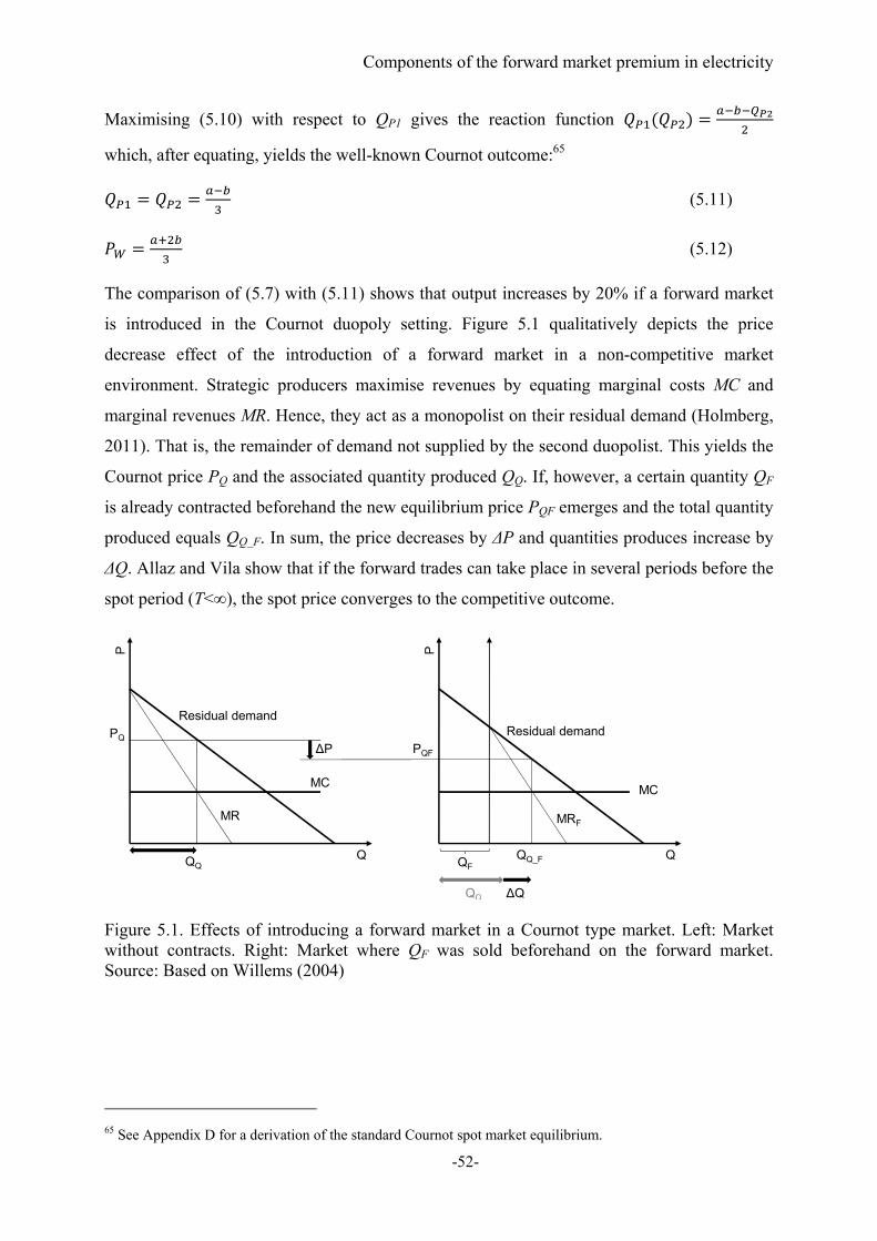
Components of the forward market premium in electricity
-52-
Maximising (5.10) with respect to QP1 gives the reaction function
which, after equating, yields the well-known Cournot outcome:65
(5.11)
(5.12)
The comparison of (5.7) with (5.11) shows that output increases by 20% if a forward market
is introduced in the Cournot duopoly setting. Figure 5.1 qualitatively depicts the price
decrease effect of the introduction of a forward market in a non-competitive market
environment. Strategic producers maximise revenues by equating marginal costs MC and
marginal revenues MR. Hence, they act as a monopolist on their residual demand (Holmberg,
2011). That is, the remainder of demand not supplied by the second duopolist. This yields the
Cournot price PQ and the associated quantity produced QQ. If, however, a certain quantity QF
is already contracted beforehand the new equilibrium price PQF emerges and the total quantity
produced equals QQ_F. In sum, the price decreases by ΔP and quantities produces increase by
ΔQ. Allaz and Vila show that if the forward trades can take place in several periods before the
spot period (T<∞), the spot price converges to the competitive outcome.
Figure 5.1. Effects of introducing a forward market in a Cournot type market. Left: Market without contracts. Right: Market where QF was sold beforehand on the forward market. Source: Based on Willems (2004)
65 See Appendix D for a derivation of the standard Cournot spot market equilibrium.
P
Q
PQ
MC
Residual demand
MR
P
Q
PQF
MC
MRF
QF
∆P
QQQQ_F
QQ ∆Q
Residual demand
Components of the forward market premium in electricity
-53-
Although this pro-competitive view of forward markets continues to be endorsed (Bushnell,
2007, et al., 2008), the theory has been challenged by several authors (e.g. Mahenc and
Salanie, 2004), when the simple two stage view of contracting is relaxed.
5.2.1.2 The Bessembinder and Lemmon model
From the other perspective, Bessembinder and Lemmon (2002), using a Taylor series
expansion of expected utility, suggest that the forward premium is a function of the variance
(negative influence) and skewness (positive influence) of spot prices. In their model NP non-
strategic symmetric generators interact with NR retailers. Demand is constant updated by a
random noise. Both producers and retailers are equally risk averse. The retail price PR is fixed.
Total costs of producer i, TCi, to produce quantity QPi are modelled as:
(5.13)
where FC are fixed costs and a and c are constants.
Spot market equilibrium
When the spot market clears demand is known with certainty. Producers sell to retailers who,
in turn, sell to final consumers. Taking into account the previously agreed forward positions
the ex post profit πPi of producer i equals
(5.14)
where PW is the wholesale spot price, QPiW and QPi
F denote the quantities sold by producer i
on the spot and forward market respectively and PF is the forward price. Clearly, generator i’s
total physical production QPi is the sum of QPiW and QPi
F.
Retailers buy the difference between their forward purchases and the realised demand on the
spot market. Retailer’s j ex post profit πRi therefore equals
(5.15)
where QRjF is the quantity sold forward (if purchased than negative) and QRj is the sold retail
quantity of retailer j.
The profit maximising quantity sold by producer i in the spot market is
(5.16)

Components of the forward market premium in electricity
-54-
Given that total physical production ∑ must equal total retail demand ∑ ≡
and considering that forward contracts are net zero supply ∑ 0 ∑ ∑
yields the equilibrium spot market price
(5.17)
Inserting (5.17) into (5.16) yields the spot market sales of producer i:
(5.18)
Forward market equilibrium
Bessembinder and Lemmon show, using the result of Hirshleifer and Subramanyam (1993),
that the optimal forward position of producer i is
,
(5.19)
and of retailer j is:
, (5.20)
where A is the coefficient of absolute risk aversion to the variance of profits in the objective
function. Positive values of A indicate that volatility risk is perceived negative.
The optimal forward position consists of two components. The first term on the right hand
side of (5.19) and (5.20) respectively is the response to the difference between the forward
price and the expected spot price (i.e. the forward premium). The second term is the quantity
sold forward to minimise the profit variance. The first term can be denoted as a speculative
position whereas the second one stems from the “pure” hedging motive (Anderson and
Danthine, 1981). Since forward contracts are net zero supply ∑ 0 the equilibrium
forward price is
, , (5.21)
where and . Bessembinder and Lemmon (2002) show that when PWx and
PWx+1 are approximated by a second order Taylor series expansion (5.21) can be stated as:
(5.22)
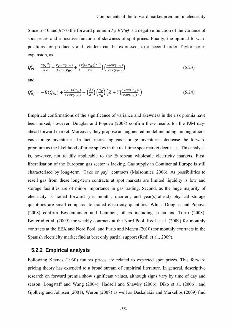
Components of the forward market premium in electricity
-55-
Since α < 0 and β > 0 the forward premium PF-E(PW) is a negative function of the variance of
spot prices and a positive function of skewness of spot prices. Finally, the optimal forward
positions for producers and retailers can be expressed, to a second order Taylor series
expansion, as
(5.23)
and
(5.24)
Empirical confirmations of the significance of variance and skewness in the risk premia have
been mixed, however. Douglas and Popova (2008) confirm these results for the PJM day-
ahead forward market. Moreover, they propose an augmented model including, among others,
gas storage inventories. In fact, increasing gas storage inventories decrease the forward
premium as the likelihood of price spikes in the real-time spot market decreases. This analysis
is, however, not readily applicable to the European wholesale electricity markets. First,
liberalisation of the European gas sector is lacking. Gas supply in Continental Europe is still
characterised by long-term “Take or pay” contracts (Maisonnier, 2006). As possibilities to
resell gas from these long-term contracts at spot markets are limited liquidity is low and
storage facilities are of minor importance in gas trading. Second, as the huge majority of
electricity is traded forward (i.e. month-, quarter-, and year(s)-ahead) physical storage
quantities are small compared to traded electricity quantities. Whilst Douglas and Popova
(2008) confirm Bessembinder and Lemmon, others including Lucia and Torro (2008),
Botterud et al. (2009) for weekly contracts at the Nord Pool, Redl et al. (2009) for monthly
contracts at the EEX and Nord Pool, and Furio and Meneu (2010) for monthly contracts in the
Spanish electricity market find at best only partial support (Redl et al., 2009).
5.2.2 Empirical analysis
Following Keynes (1930) futures prices are related to expected spot prices. This forward
pricing theory has extended to a broad stream of empirical literature. In general, descriptive
research on forward premia show significant values, although signs vary by time of day and
season. Longstaff and Wang (2004), Hadsell and Shawky (2006), Diko et al. (2006), and
Gjolberg and Johnsen (2001), Weron (2008) as well as Daskalakis and Markellos (2009) find
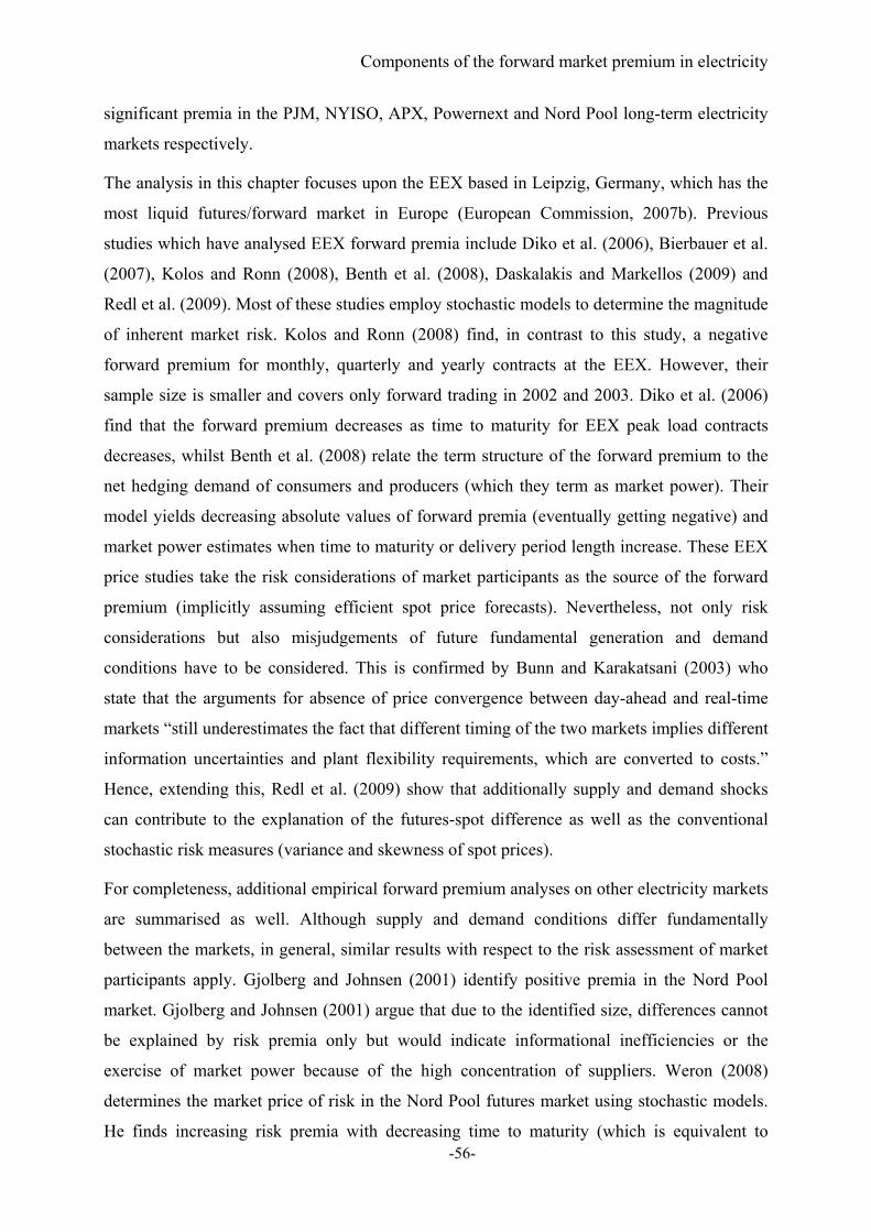
Components of the forward market premium in electricity
-56-
significant premia in the PJM, NYISO, APX, Powernext and Nord Pool long-term electricity
markets respectively.
The analysis in this chapter focuses upon the EEX based in Leipzig, Germany, which has the
most liquid futures/forward market in Europe (European Commission, 2007b). Previous
studies which have analysed EEX forward premia include Diko et al. (2006), Bierbauer et al.
(2007), Kolos and Ronn (2008), Benth et al. (2008), Daskalakis and Markellos (2009) and
Redl et al. (2009). Most of these studies employ stochastic models to determine the magnitude
of inherent market risk. Kolos and Ronn (2008) find, in contrast to this study, a negative
forward premium for monthly, quarterly and yearly contracts at the EEX. However, their
sample size is smaller and covers only forward trading in 2002 and 2003. Diko et al. (2006)
find that the forward premium decreases as time to maturity for EEX peak load contracts
decreases, whilst Benth et al. (2008) relate the term structure of the forward premium to the
net hedging demand of consumers and producers (which they term as market power). Their
model yields decreasing absolute values of forward premia (eventually getting negative) and
market power estimates when time to maturity or delivery period length increase. These EEX
price studies take the risk considerations of market participants as the source of the forward
premium (implicitly assuming efficient spot price forecasts). Nevertheless, not only risk
considerations but also misjudgements of future fundamental generation and demand
conditions have to be considered. This is confirmed by Bunn and Karakatsani (2003) who
state that the arguments for absence of price convergence between day-ahead and real-time
markets “still underestimates the fact that different timing of the two markets implies different
information uncertainties and plant flexibility requirements, which are converted to costs.”
Hence, extending this, Redl et al. (2009) show that additionally supply and demand shocks
can contribute to the explanation of the futures-spot difference as well as the conventional
stochastic risk measures (variance and skewness of spot prices).
For completeness, additional empirical forward premium analyses on other electricity markets
are summarised as well. Although supply and demand conditions differ fundamentally
between the markets, in general, similar results with respect to the risk assessment of market
participants apply. Gjolberg and Johnsen (2001) identify positive premia in the Nord Pool
market. Gjolberg and Johnsen (2001) argue that due to the identified size, differences cannot
be explained by risk premia only but would indicate informational inefficiencies or the
exercise of market power because of the high concentration of suppliers. Weron (2008)
determines the market price of risk in the Nord Pool futures market using stochastic models.
He finds increasing risk premia with decreasing time to maturity (which is equivalent to

Components of the forward market premium in electricity
-57-
decreasing forward premia over time). Bunn (2006) identifies positive premia for peak hours
when comparing the UK day ahead and prompt market and the week ahead and day ahead
market which is explained by a higher willingness to pay day ahead of the demand side in
order to avoid the intra-day market volatility (and vice versa for the off peak hours).
Similarly, Longstaff and Wang (2004), Hadsell and Shawky (2006), Diko et al. (2006), and
Daskalakis and Markellos (2009) find significant risk premia in the PJM, NYISO, APX,
Powernext and Nord Pool long-term electricity markets respectively.
5.3 Market setting and Initial Data Analysis
This analysis focuses on month-ahead futures prices for several reasons. Firstly, this is the
most liquid contract and most price data is available for futures with monthly delivery
periods. Secondly, due to the near-term delivery period, the forecast errors of market
participants should, on average, be low for up to one month ahead.66 More specifically, prices
on the last trading day before the delivery month are considered only due to the limited
availability of fundamental data (e.g. supply and demand data).
Futures at the EEX are settled financially. For baseload the underlying is the mean of all
hourly spot prices during the delivery period. For peak load the underlying is the Phelix peak
load index, which is the mean of the peak hours from 8:00am to 8:00 pm from Monday to
Friday during the delivery period.67
As discussed in Chapter 3 the European electricity market is still characterised by several
(regional or national) wholesale price areas. As the Central/Western European power market
is, however, formed by several countries fundamental supply and demand conditions in all of
these countries have to be considered even if the EEX is the leading exchange in this extended
region. Figure 5.2 shows the evolution of monthly averages of spot peak load prices as well as
month-ahead peak load prices, as reported on the last trading day for delivery during the
plotted month, at the EEX from October 2003 to January 2010.68 Spot and forward prices
were rising continuously until early 2006. Since fossil fuelled power plants constitute the
price setting technologies in the EEX market, increasing power prices mainly reflected rising
66 Still, a spot price forecast covering an entire month may yield significant errors. I will deal with this issue in the following sections. 67 http://www.eex.com/en 68 In Figure 5.2 the depicted forward price at, e.g. October 2003, was the settlement price of the month-ahead peak load futures on 30 September 2003 for a delivery during peak hours in October 2003.

Components of the forward market premium in electricity
-58-
primary energy prices. The increase observed during 2005 was partly due to the
commencement of carbon trading through the EU-ETS.
Figure 5.2. Evolution of monthly averages of peak load spot prices (black) and peak load month-ahead futures prices on the last trading day (grey) at the EEX from October 2003 to January 2010. Source: EEX
Figure 5.3 presents descriptive statistics for daily EEX base and peak load spot prices from
October 2003 to January 2010. The price series are non-normal, positively skewed and show a
high kurtosis. As expected, the peak load price series is more volatile than the baseload series
(in terms of both the standard deviation and the coefficient of variation). It is this distribution
which faces the market participants with a forecasting problem of future spot prices.
Moreover, risk-averse agents have an incentive to reduce their risk exposure by trading on the
forward market. As will be shown in the following, the willingness to pay in order to reduce
this risk exposure is significant.
0
20
40
60
80
100
120
140
[€/M
Wh]
Month ahead futures price
Spot peak price
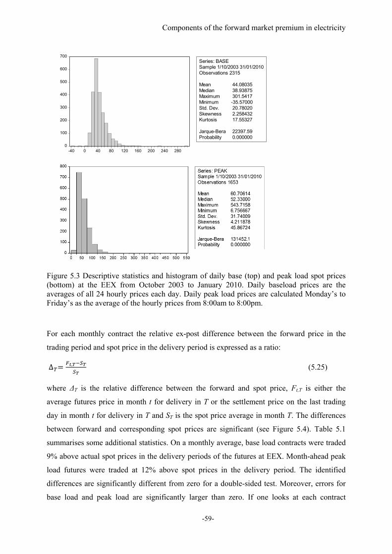
Components of the forward market premium in electricity
-59-
Figure 5.3 Descriptive statistics and histogram of daily base (top) and peak load spot prices (bottom) at the EEX from October 2003 to January 2010. Daily baseload prices are the averages of all 24 hourly prices each day. Daily peak load prices are calculated Monday’s to Friday’s as the average of the hourly prices from 8:00am to 8:00pm.
For each monthly contract the relative ex-post difference between the forward price in the
trading period and spot price in the delivery period is expressed as a ratio:
∆ , (5.25)
where ΔT is the relative difference between the forward and spot price, Ft,T is either the
average futures price in month t for delivery in T or the settlement price on the last trading
day in month t for delivery in T and ST is the spot price average in month T. The differences
between forward and corresponding spot prices are significant (see Figure 5.4). Table 5.1
summarises some additional statistics. On a monthly average, base load contracts were traded
9% above actual spot prices in the delivery periods of the futures at EEX. Month-ahead peak
load futures were traded at 12% above spot prices in the delivery period. The identified
differences are significantly different from zero for a double-sided test. Moreover, errors for
base load and peak load are significantly larger than zero. If one looks at each contract
0
100
200
300
400
500
600
700
-40 0 40 80 120 160 200 240 280
Series: BASESample 1/10/2003 31/01/2010Observations 2315
Mean 44.08035Median 38.93875Maximum 301.5417Minimum -35.57000Std. Dev. 20.78020Skewness 2.258432Kurtosis 17.55327
Jarque-Bera 22397.59Probability 0.000000
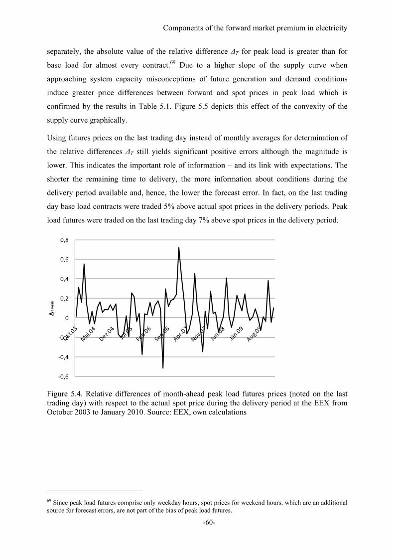
Components of the forward market premium in electricity
-60-
separately, the absolute value of the relative difference ΔT for peak load is greater than for
base load for almost every contract.69 Due to a higher slope of the supply curve when
approaching system capacity misconceptions of future generation and demand conditions
induce greater price differences between forward and spot prices in peak load which is
confirmed by the results in Table 5.1. Figure 5.5 depicts this effect of the convexity of the
supply curve graphically.
Using futures prices on the last trading day instead of monthly averages for determination of
the relative differences ΔT still yields significant positive errors although the magnitude is
lower. This indicates the important role of information – and its link with expectations. The
shorter the remaining time to delivery, the more information about conditions during the
delivery period available and, hence, the lower the forecast error. In fact, on the last trading
day base load contracts were traded 5% above actual spot prices in the delivery periods. Peak
load futures were traded on the last trading day 7% above spot prices in the delivery period.
Figure 5.4. Relative differences of month-ahead peak load futures prices (noted on the last trading day) with respect to the actual spot price during the delivery period at the EEX from October 2003 to January 2010. Source: EEX, own calculations
69 Since peak load futures comprise only weekday hours, spot prices for weekend hours, which are an additional source for forecast errors, are not part of the bias of peak load futures.
‐0,6
‐0,4
‐0,2
0
0,2
0,4
0,6
0,8
ΔT Peak
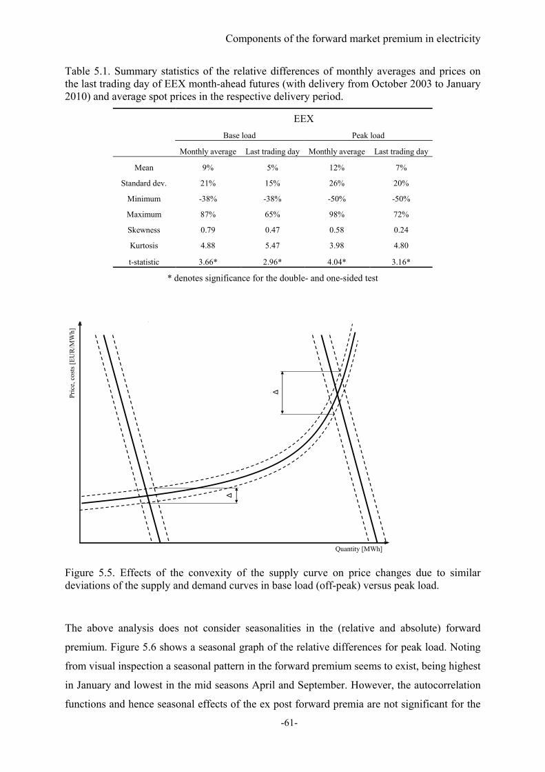
Components of the forward market premium in electricity
-61-
Table 5.1. Summary statistics of the relative differences of monthly averages and prices on the last trading day of EEX month-ahead futures (with delivery from October 2003 to January 2010) and average spot prices in the respective delivery period.
Figure 5.5. Effects of the convexity of the supply curve on price changes due to similar deviations of the supply and demand curves in base load (off-peak) versus peak load.
The above analysis does not consider seasonalities in the (relative and absolute) forward
premium. Figure 5.6 shows a seasonal graph of the relative differences for peak load. Noting
from visual inspection a seasonal pattern in the forward premium seems to exist, being highest
in January and lowest in the mid seasons April and September. However, the autocorrelation
functions and hence seasonal effects of the ex post forward premia are not significant for the
EEX
Base load Peak load
Monthly average Last trading day Monthly average Last trading day
Mean 9% 5% 12% 7%
Standard dev. 21% 15% 26% 20%
Minimum -38% -38% -50% -50%
Maximum 87% 65% 98% 72%
Skewness 0.79 0.47 0.58 0.24
Kurtosis 4.88 5.47 3.98 4.80
t-statistic 3.66* 2.96* 4.04* 3.16*
* denotes significance for the double- and one-sided test
Pri
ce, c
osts
[EU
R/M
Wh]
Quantity [MWh]
∆
∆
t
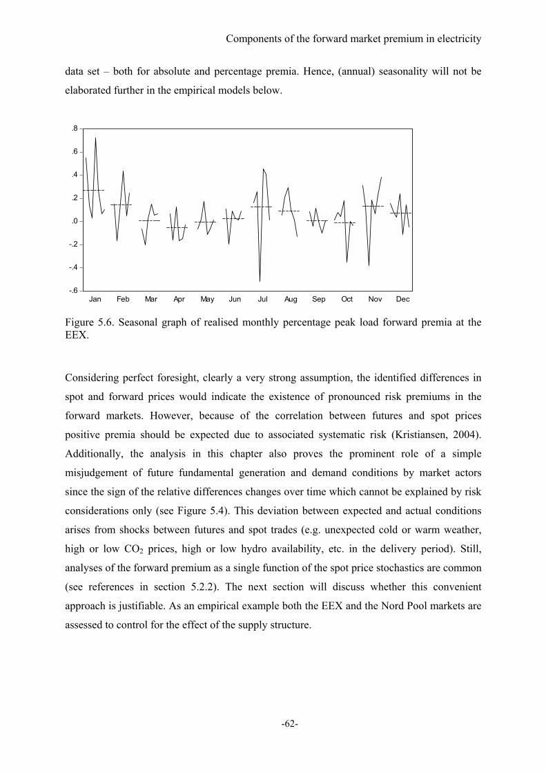
Components of the forward market premium in electricity
-62-
data set – both for absolute and percentage premia. Hence, (annual) seasonality will not be
elaborated further in the empirical models below.
Figure 5.6. Seasonal graph of realised monthly percentage peak load forward premia at the EEX.
Considering perfect foresight, clearly a very strong assumption, the identified differences in
spot and forward prices would indicate the existence of pronounced risk premiums in the
forward markets. However, because of the correlation between futures and spot prices
positive premia should be expected due to associated systematic risk (Kristiansen, 2004).
Additionally, the analysis in this chapter also proves the prominent role of a simple
misjudgement of future fundamental generation and demand conditions by market actors
since the sign of the relative differences changes over time which cannot be explained by risk
considerations only (see Figure 5.4). This deviation between expected and actual conditions
arises from shocks between futures and spot trades (e.g. unexpected cold or warm weather,
high or low CO2 prices, high or low hydro availability, etc. in the delivery period). Still,
analyses of the forward premium as a single function of the spot price stochastics are common
(see references in section 5.2.2). The next section will discuss whether this convenient
approach is justifiable. As an empirical example both the EEX and the Nord Pool markets are
assessed to control for the effect of the supply structure.
-.6
-.4
-.2
.0
.2
.4
.6
.8
Jan Feb Mar Apr May Jun Jul Aug Sep Oct Nov Dec
Components of the forward market premium in electricity
-63-
5.4 Excursus: Is the forward premium explained well by stochastic
properties of spot prices?
5.4.1 Testing the Bessembinder and Lemmon model 70
The following equation is estimated by OLS to test the predictions of the model of
Bessembinder and Lemmon (2002):71
tttTTt SSkewbSVarbbSF )()( 321, (5.26)
where Ft,T-ST is the ex post forward premium, Ft,T is the futures price in t for delivery in
month T, ST is the spot price average in month T, Var(St) is the variance of daily spot prices in
month t and Skew(St) is the skewness of daily spot prices in month t.
For monthly averages of futures prices strong serial correlation in the residuals is noticed
from diagnostic checks which could be constituted to the fact that the data represent monthly
averages. Therefore, this regression is tested with the definition of the forward price on the
last trading day. Results for corresponding forward premia are shown in Table 5.2. As can be
seen, serial correlation is no longer present in the residuals.
At the EEX the (positive) influence of the variance of baseload spot prices in the trading
period of the futures contracts on forward premia is significant on a 10% level. The skewness
of spot prices is not significant. For EEX peak load premia, similarly, a significant variance
coefficient is obtained which points to its relevance but does not correspond to the
interpretation in the Bessembinder and Lemmon (2002) model. The regression coefficient of
the skewness of spot prices is positive for peak load but not significant. The models can only
explain 7% (baseload model) and 4% (peak load model) of the variance of the forward
premium. However, as peak load prices are very sensitive to changes in a variety of
parameters – many not considered in model (5.26) – a lower performance of the peak load
model is to be expected. Due to the asymmetry of spot prices and occasional spikes the
hypothesis of normally distributed error terms has to be rejected although other diagnostic test
statistics of the residuals are not significant.
70 Based on Redl et al. (2009). 71 Using the spot price distributions for month t (the trading month) is an intentional choice. The analytical result of Bessembinder and Lemmon is that the premium depends on the spot price distribution in month T. Hence, the model of BL assumes rational expectations. The analysis in this thesis is based on testing an adaptive expectation formation instead. Hence month t values are used. All variables in the empirical model are therefore observable for the market participants. Douglas and Popova (2008) use a similar "adaptive" model. Moreover, estimating (5.26) with month T values would bring about the problem of overlapping observations. Running (5.26) nevertheless with month T values does not conform to the results of BL as well.
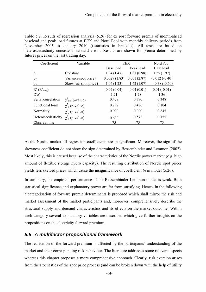
Components of the forward market premium in electricity
-64-
Table 5.2. Results of regression analysis (5.26) for ex post forward premia of month-ahead baseload and peak load futures at EEX and Nord Pool with monthly delivery periods from November 2003 to January 2010 (t-statistics in brackets). All tests are based on heteroscedasticity consistent standard errors. Results are shown for premia determined by futures prices on the last trading day.
At the Nordic market all regression coefficients are insignificant. Moreover, the sign of the
skewness coefficient do not show the sign determined by Bessembinder and Lemmon (2002).
Most likely, this is caused because of the characteristics of the Nordic power market (e.g. high
amount of flexible storage hydro capacity). The resulting distribution of Nordic spot prices
yields less skewed prices which cause the insignificance of coefficient b3 in model (5.26).
In summary, the empirical performance of the Bessembinder Lemmon model is weak. Both
statistical significance and explanatory power are far from satisfying. Hence, in the following
a categorisation of forward premia determinants is proposed which shall mirror the risk and
market assessment of the market participants and, moreover, comprehensively describe the
structural supply and demand characteristics and its effects on the market outcome. Within
each category several explanatory variables are described which give further insights on the
propositions on the electricity forward premium.
5.5 A multifactor propositional framework
The realisation of the forward premium is affected by the participants’ understanding of the
market and their corresponding risk behaviour. The literature addresses some relevant aspects
whereas this chapter proposes a more comprehensive approach. Clearly, risk aversion arises
from the stochastics of the spot price process (and can be broken down with the help of utility
Coefficient Variable Nord PoolBase load Peak load Base load
b1 Constant 1.34 (1.47) 1.81 (0.98) 1.25 (1.97)b2 Variance spot price t 0.0027 (1.83) 0.001 (2.87) -0.012 (-0.40)b3 Skewness spot price t 1.04 (1.23) 1.42 (1.07) -0.38 (-0.60)
R2 (R2corr) 0.07 (0.04) 0.04 (0.01) 0.01 (-0.01)
DW 1.71 1.78 1.36Serial correlation χ2
12 (p-value) 0.478 0.370 0.348
Functional form χ21 (p-value) 0.292 0.486 0.104
Normality χ22 (p-value) 0.000 0.000 0.845
Heteroscedasticity χ21 (p-value) 0.630 0.572 0.155
Observations 75 75 75
EEX
Components of the forward market premium in electricity
-65-
functions to aversion to higher moments of the price distribution). But also fundamentals are
expected to cause variations in the market price of risk. The margin, for example, constitutes a
well known property of the spot price. Hence, the margin is expected to be a part of the risk
assessment. Similarly, input fuel prices should affect the price of risk. Furthermore, the
participants’ perception of commodity markets in general can influence their assessment of
the commodity electricity as well as behavioural biases (e.g. caused by employing heuristics
or anchoring decisions to past events).72
This chapter therefore seeks to embed and extend the various factors introduced in previous
work into a more comprehensive analysis. In doing this the forward premium components are
organised into a taxonomy of fundamental influences, behavioural effects, market conduct,
dynamic effects and shock effects. Specifically the following propositions are addressed:
Fundamental influences
The fundamental drivers (Bunn, 2004, Weron, 2006) of power prices are demand, marginal
costs (fuel and carbon prices), and scarcity (margin). Demand presents a particular problem.
Because of endogeniety concerns and the difficulty of specifying demand for a market with a
high degree of interconnection to neighbours, such as EEX, an average central European
temperature was taken as a proxy. This proved not to be significant, however. An analysis of
the effect of temperature surprises (actual monthly average in the delivery month minus long
term ex ante monthly average) did turn out to be significant. Nevertheless, the series on
temperature data has several shortcomings. Hence, demand measured by its proxy
temperature is not considered in the model below. The robustness analysis in section 5.6.3.1
will elaborate on this issue. Daskalakis and Markellos (2009) find that EEX forward premia
can be partly explained by the volatility of CO2 spot price returns. This analysis does not
consider CO2 prices, since the volatility of electricity spot prices, which, in turn, are
influenced by carbon prices, is included.73 For specific propositions, therefore only fuels and
scarcity are considered.
72 See Ricciardi (2008) for a review of behavioural decision theory. 73 Reassuringly, the inclusion of carbon price volatility resulted in an insignificant regression coefficient. Apart from the volatility of CO2 prices affecting the electricity forward premium the latter could also be influenced by the premium in the CO2 market. However, there are no month-ahead CO2 contracts traded.
Components of the forward market premium in electricity
-66-
Fuels and their risk premia: Proposition: An increase in the gas forward premium is
expected to increase the electricity forward premium, whereas the effect is anticipated
to be more pronounced in peak load compared to base load.
Given the high importance of fossil fuelled generation technologies in the EEX
market, the premium prevailing in the electricity contract market should be directly
influenced by the premium in the gas market.74 This influence can be motivated by
either risk management considerations, since – assuming gas fired price setting
technologies – the realised spark spread constitutes the risk exposure of a generator
having contracted gas, or the forecast errors of the respective market participant.
Scarcity: Proposition: A negative relationship between the observed reserve margin
and the forward premium is expected75.
A reduction in the reserve margin indicates relative scarcity and one would expect that
this leads to a higher propensity for shocks to induce greater price volatility and
spikes. Given an adaptive expectations adjustment by market participants, a perceived
decreasing margin in the spot market may cause expected spot prices and therefore
forward prices and, correspondingly, premia to increase.76
Behavioural effects
Adaptive expectation formation with respect to the risk assessment of the market participants
is postulated, as motivated by high correlations between current spot and forward electricity
prices and the adaptive heuristics that research in behavioural finance indicates is likely to
prevail (e.g., Ricciardi, 2008). It is plausible that spot market realisations in the trading month
of the forward contract will be used by agents as proxies for the anticipated realisations in the
delivery month as spot price forecasts for a delivery period comprising one month ahead
prove to be elusive (for research aiming to model expectation behaviour and market
participants alike). Hence, a link between current long and short term prices appears not
surprising. Similarly, the risk assessment of market participants considers current market
74 The price setting technologies in the peak load segment are gas fired. For base load, the coal market could similarly influence the electricity market. Still, there exists no coal spot market in the EEX region which precludes the calculation of corresponding forward premia. Moreover, with the introduction of carbon trading, gas fired power plants have gained increased importance also in the base load segment. 75 The reserve margin as ratio of generation and demand constitutes a measurement for scarcity in the electricity supply system. 76 It would be reasonable to suggest a nonlinear effect of the reserve margin given the convexity of the supply curve. However, the results did not differ when linear margin terms are replaced by quadratic ones.
Components of the forward market premium in electricity
-67-
developments. Thus, in the following models the realisations of the relevant assessment
parameters in the spot market in the trading month of the forward contract are used as proxies
for the anticipated spot distribution realisations in the delivery month.77
Higher moments: Proposition: Higher central moments of the spot price distribution
(variance, skewness and kurtosis) are of importance for the risk assessment of market
actors.
The capital asset pricing model and, correspondingly, the mean-variance utility
assumption, are widely used for the assessment of securities markets (Newbery, 1988).
This popular approach has spilled over to plenty of analyses in the field of electricity
forward markets and, especially, electricity forward premia. The influential work of
Bessembinder and Lemmon (2002) considers agents to be non-strategic, risk averse
utility maximisers, but their main result neglects higher moments beyond variance and
skewness in the Taylor series expansion. Given the increasing interest in fat tails and
aversion to extreme outcomes, it is plausible that a positive influence of the kurtosis of
spot prices on the premium could be expected.
Positively skewed spot prices increase the hedging demand of retailers given fixed
retail prices. On the other hand, spot price spikes represent opportunity costs of
generators having sold forward. Both factors contribute to a positive forward
premium. Hence the regression coefficient associated with the skewness should show
a positive sign. The influence of the variance of spot prices on the forward premium is,
however, not clear cut. Bessembinder and Lemmon (2002) predict a negative effect. It
could be argued however, that, due to the convexity of the supply curve, shocks that
create high skewness and volatility are very similar and therefore in the risk premia
regressions, these two moments should have similar signs.
Spikes: Proposition: The forward premium increases due to the occurrence of spikes
in the spot market.
It is plausible that recent spike episodes may induce greater risk aversion. Dummy
variables which account for the occurrence of spikes may allow a more subtle
representation of this compared to the skewness and kurtosis measures. Different
degrees of spikiness respectively thresholds can be defined (mean plus one, 1.5, two,
2.5 and three standard deviations, Weron, 2006). The relevant spot price aggregation
77 In the light of adaptive expectations a further natural risk assessment parameter would be the corresponding realisation in the spot market of the same delivery month a year ago. Still, all 12-month lagged variables turned out to be statistically insignificant in the models.

Components of the forward market premium in electricity
-68-
level for estimating spikes at the EEX is the daily base or peak load spot price average
(Phelix Base, Phelix Peak), since the underlying of monthly futures contracts is the
monthly average of the Phelix day indices. Given positively skewed spot prices a
positive influence of the spike count variable on the premium is expected.
Oil market volatility: Proposition: Increased volatility in the oil market increases the
electricity forward premium.
Due to the dominance of oil prices in the energy commodity bundle and its sentiment
effect for energy commodities in general, it is plausible that electricity market agents
are influenced by activity in the oil market.78 Hence, a regression coefficient
associated with oil market volatility would be expected to show a positive sign.
Market conduct
Market power: Proposition: The exercise of market power in the spot market
positively influences the forward premium.
Theory is mixed on the interaction of market power and forward contracting. I have
already referred to the work of Allaz and Vila (1993), which suggests that forward
contracting mitigates the exercise of market power in the spot market. On the other
hand, the model of Robinson and Baniak (2002) including oligopolistic risk neutral
generators and risk averse retailers suggests that the generators increase the spot
market volatility in order to increase the forward premium in contracts. Furthermore, it
is plausible to argue, similarly to Anderson and Hu (2008), that producers who can
increase spot market prices demand a higher premium to contract forward and that
buyers see generator market power as an additional risk factor which increases their
willingness to pay forward premia.
The estimation of reliable forward market concentration proxy variables, which would
allow empirical insights into market power, is, however, quite elusive in the absence
of detailed contract data. On the other hand, estimated base load and peak load price
mark ups above marginal cost estimates for the spot market can be included in the
analysis. Figure 5.7 below depicts the evolution of EEX spot prices and estimated
monthly averages of marginal costs in the regional EU4 market from 2003-2009. The
corresponding mark up variable, defined as the ratio of the price-cost-difference to the
78 Even though oil fired power plants are very rarely dispatched.
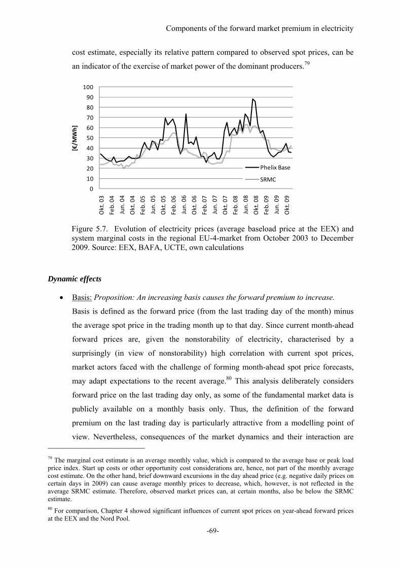
Components of the forward market premium in electricity
-69-
cost estimate, especially its relative pattern compared to observed spot prices, can be
an indicator of the exercise of market power of the dominant producers.79
Figure 5.7. Evolution of electricity prices (average baseload price at the EEX) and system marginal costs in the regional EU-4-market from October 2003 to December 2009. Source: EEX, BAFA, UCTE, own calculations
Dynamic effects
Basis: Proposition: An increasing basis causes the forward premium to increase.
Basis is defined as the forward price (from the last trading day of the month) minus
the average spot price in the trading month up to that day. Since current month-ahead
forward prices are, given the nonstorability of electricity, characterised by a
surprisingly (in view of nonstorability) high correlation with current spot prices,
market actors faced with the challenge of forming month-ahead spot price forecasts,
may adapt expectations to the recent average.80 This analysis deliberately considers
forward price on the last trading day only, as some of the fundamental market data is
publicly available on a monthly basis only. Thus, the definition of the forward
premium on the last trading day is particularly attractive from a modelling point of
view. Nevertheless, consequences of the market dynamics and their interaction are 79 The marginal cost estimate is an average monthly value, which is compared to the average base or peak load price index. Start up costs or other opportunity cost considerations are, hence, not part of the monthly average cost estimate. On the other hand, brief downward excursions in the day ahead price (e.g. negative daily prices on certain days in 2009) can cause average monthly prices to decrease, which, however, is not reflected in the average SRMC estimate. Therefore, observed market prices can, at certain months, also be below the SRMC estimate. 80 For comparison, Chapter 4 showed significant influences of current spot prices on year-ahead forward prices at the EEX and the Nord Pool.
0
10
20
30
40
50
60
70
80
90
100
Okt. 03
Feb. 04
Jun. 04
Okt. 04
Feb. 05
Jun. 05
Okt. 05
Feb. 06
Jun. 06
Okt. 06
Feb. 07
Jun. 07
Okt. 07
Feb. 08
Jun. 08
Okt. 08
Feb. 09
Jun. 09
Okt. 09
[€/M
Wh]
Phelix Base
SRMC
Components of the forward market premium in electricity
-70-
considered in this analysis. Specifically, the tie between spot and forward prices is also
reflected in the basis. A significant influence of the basis therefore gives further
insight into the expectation formation of the market participants. An increasing basis is
expected to increase the forward premium.
Seasonality: Seasonal effects, above those which can be fundamentally modelled (e.g.
the system margin), have been observed in other studies (Weron, 2008) of the forward
premium. However, due to the statistical insignificance reported in section 5.3,
(annual) seasonality will not be considered in the empirical analysis below.
Shocks
Proposition: Margin shocks positively influence the forward premium.
To be able to account for supply and demand shocks between forward trades and future spot
trades a margin shock variable is introduced. Specifically, the margin shock variable captures
the ratio between total generation and actual electricity consumption in the relevant regional
market. This combined approach has been chosen to avoid long-term trend effects of a
separate consumption and generation representation. If, ceteris paribus, consumption is
unexpectedly high in the delivery month spot prices should exceed forward prices due to a
decreasing margin. On the other hand, if, ceteris paribus, total generation rises unexpectedly
spot prices should fall below forward prices since the supply curve is shifted to the right.
Hence, the regression coefficient associated with the realised margin is expected to show a
positive sign.
Summary of propositions
Table 5.3 summarises the above propositions on the effects of forward premia components
and respective proxy variables. Apart from the margin shock, all variables are observable for
the market participants on the forward trading day.

Components of the forward market premium in electricity
-71-
Table 5.3. Summary of forward premia determinants. * denotes that the respective variables are observable for market participants on the forward trading day.
In the following reduced form models aiming to give insights on the above propositions are
presented.
5.6 A model of the ex post forward premium
This section develops reduced form models to give insights on the above propositions.
Furthermore, the analysis assumes myopic expectations in the sense that the market
participants are influenced by current and historic events on the spot market. These events, in
turn, contribute to the risk and market assessment of the agents and, hence, to the forward
premium. All parameters except the margin shock are observable for the market participants
on the last trading day of month t.81
5.6.1 Base load premium model
Sequentially minimising the AIC criterion, pursuing a general-to-specific model identification
characterised by all variables discussed in section 5.5, yields the following equation for the ex
post baseload forward premium:
81 For comparison, Douglas and Popova (2008) also partly assume adaptive expectations in their model – represented in particular by one period lagged values of variance and skewness of spot prices and gas storage levels.
Effect on forward
premium Proxy variable
Fundamentals*
Premia in fuels + Month ahead gas forward premium
Scarcity - Reserve margin: Ratio generation/consumption in the regional market Behavioural effects*
Variance + Coefficient of variation of spot price
Skewness + Skewness of spot price
Kurtosis + Kurtosis of spot price
Spikes + Count spikes outside 1, 1.5, 2, 2.5, 3 standard deviations of mean spot
Oil volatility + Coefficient of variation of Brent oil spot price
Conduct* Spot market
power + Fundamental cost mark up estimate for regional spot market
Dynamics*
Basis + Difference of forward price and spot price average in trading month
Shocks
Margin shocks + Change in supply margin during delivery month
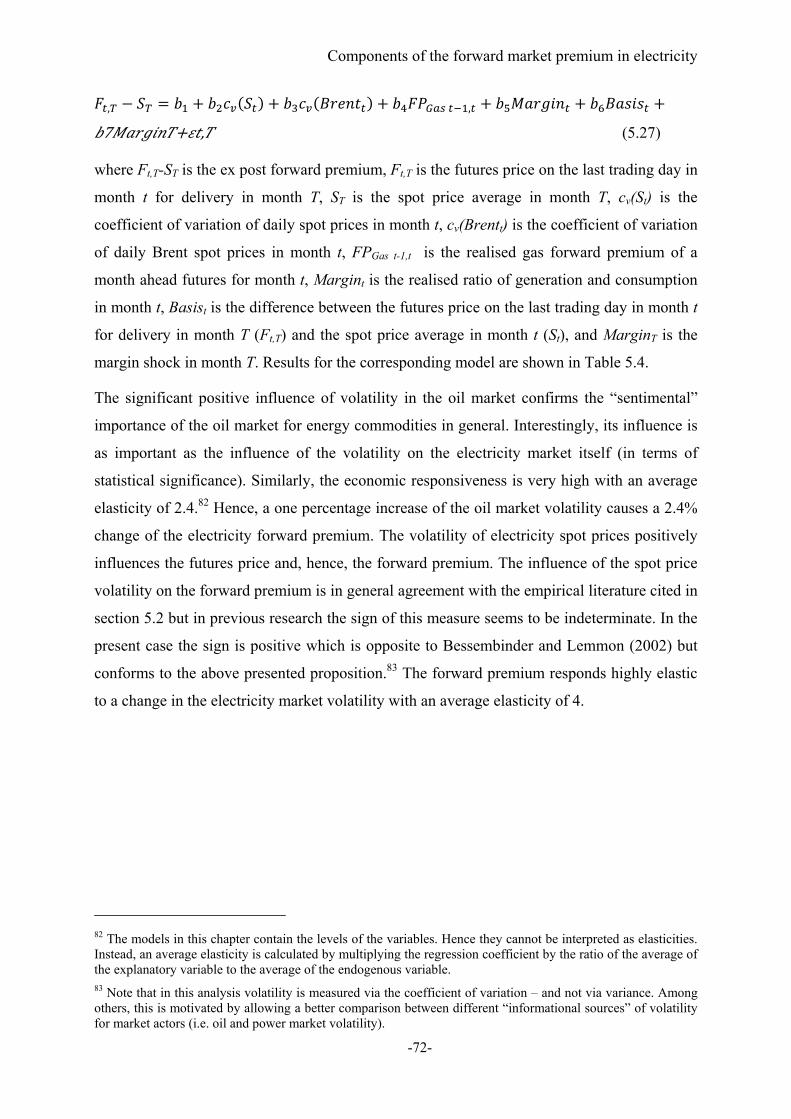
Components of the forward market premium in electricity
-72-
, ,
7 , (5.27)
where Ft,T-ST is the ex post forward premium, Ft,T is the futures price on the last trading day in
month t for delivery in month T, ST is the spot price average in month T, cv(St) is the
coefficient of variation of daily spot prices in month t, cv(Brentt) is the coefficient of variation
of daily Brent spot prices in month t, FPGas t-1,t is the realised gas forward premium of a
month ahead futures for month t, Margint is the realised ratio of generation and consumption
in month t, Basist is the difference between the futures price on the last trading day in month t
for delivery in month T (Ft,T) and the spot price average in month t (St), and MarginT is the
margin shock in month T. Results for the corresponding model are shown in Table 5.4.
The significant positive influence of volatility in the oil market confirms the “sentimental”
importance of the oil market for energy commodities in general. Interestingly, its influence is
as important as the influence of the volatility on the electricity market itself (in terms of
statistical significance). Similarly, the economic responsiveness is very high with an average
elasticity of 2.4.82 Hence, a one percentage increase of the oil market volatility causes a 2.4%
change of the electricity forward premium. The volatility of electricity spot prices positively
influences the futures price and, hence, the forward premium. The influence of the spot price
volatility on the forward premium is in general agreement with the empirical literature cited in
section 5.2 but in previous research the sign of this measure seems to be indeterminate. In the
present case the sign is positive which is opposite to Bessembinder and Lemmon (2002) but
conforms to the above presented proposition.83 The forward premium responds highly elastic
to a change in the electricity market volatility with an average elasticity of 4.
82 The models in this chapter contain the levels of the variables. Hence they cannot be interpreted as elasticities. Instead, an average elasticity is calculated by multiplying the regression coefficient by the ratio of the average of the explanatory variable to the average of the endogenous variable. 83 Note that in this analysis volatility is measured via the coefficient of variation – and not via variance. Among others, this is motivated by allowing a better comparison between different “informational sources” of volatility for market actors (i.e. oil and power market volatility).
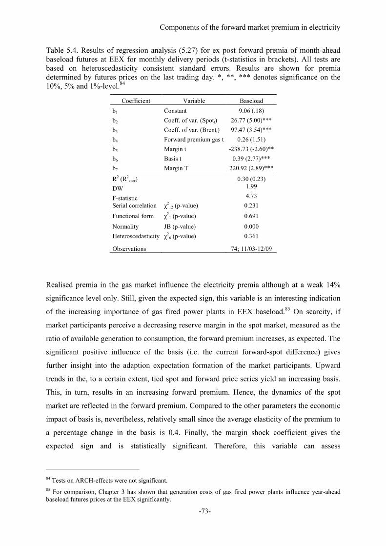
Components of the forward market premium in electricity
-73-
Table 5.4. Results of regression analysis (5.27) for ex post forward premia of month-ahead baseload futures at EEX for monthly delivery periods (t-statistics in brackets). All tests are based on heteroscedasticity consistent standard errors. Results are shown for premia determined by futures prices on the last trading day. *, **, *** denotes significance on the 10%, 5% and 1%-level.84
Realised premia in the gas market influence the electricity premia although at a weak 14%
significance level only. Still, given the expected sign, this variable is an interesting indication
of the increasing importance of gas fired power plants in EEX baseload.85 On scarcity, if
market participants perceive a decreasing reserve margin in the spot market, measured as the
ratio of available generation to consumption, the forward premium increases, as expected. The
significant positive influence of the basis (i.e. the current forward-spot difference) gives
further insight into the adaption expectation formation of the market participants. Upward
trends in the, to a certain extent, tied spot and forward price series yield an increasing basis.
This, in turn, results in an increasing forward premium. Hence, the dynamics of the spot
market are reflected in the forward premium. Compared to the other parameters the economic
impact of basis is, nevertheless, relatively small since the average elasticity of the premium to
a percentage change in the basis is 0.4. Finally, the margin shock coefficient gives the
expected sign and is statistically significant. Therefore, this variable can assess
84 Tests on ARCH-effects were not significant. 85 For comparison, Chapter 3 has shown that generation costs of gas fired power plants influence year-ahead baseload futures prices at the EEX significantly.
Coefficient Variable Baseload
b1 Constant 9.06 (.18)
b2 Coeff. of var. (Spott) 26.77 (5.00)***
b3 Coeff. of var. (Brentt) 97.47 (3.54)***
b4 Forward premium gas t 0.26 (1.51)
b5 Margin t -238.73 (-2.60)**
b6 Basis t 0.39 (2.77)***
b7 Margin T 220.92 (2.89)***
R2 (R2corr) 0.30 (0.23)
DW 1.99
F-statistic 4.73
Serial correlation χ212 (p-value) 0.231
Functional form χ21 (p-value) 0.691
Normality JB (p-value) 0.000
Heteroscedasticity χ26 (p-value) 0.361
Observations 74; 11/03-12/09

Components of the forward market premium in electricity
-74-
misjudgements of future supply and demand conditions and captures some of the forecast
error part of the forward premium defined by equation (5.1).86
5.6.2 Peak load premium model
A similar procedure to the above described one yields the following equation for the ex post
peak load forward premium:
, ,
, (5.28)
where Ft,T-ST is the ex post forward premium, Ft,T is the peak load futures price on the last
trading day in month t for delivery during peak hours in month T, ST is the peak load spot
price average in month T, Skew(St) is the skewness of daily spot prices in month t, Spike2sd t is
the count of spikes outside of 2 standard deviations of the mean spot price in month t,
FPGas t-1,t is the realised gas forward premium of a month ahead futures for month t, Spot
market powert is the ratio of the spot price in month t and the fundamental marginal cost
estimate for month t, Margint is the ratio of regional generation and demand in month t, Basist
is the difference between the futures price on the last trading day in month t for delivery in
month T (Ft,T) and the spot price average in month t (St), and MarginT is the margin shock in
month T. Results for the corresponding model are shown in Table 5.5.
Realised premia in the gas market, as expected, have a significantly positive effect on the
electricity peak load premia. The price setting technologies in peak load hours are, in fact, gas
fired power plants. The significant positive influence gas market confirms the importance of
these generation technologies although the electricity premium reacts in economic terms
inelastically to changes in the gas premium with an elasticity of 0.15. The skewness of spot
prices positively influences forward premia for peak load. If the observed spot price skewness
increases by one percentage point the forward premium increases by 0.4%. Positively skewed
spot prices increase the hedging demand of retailers given fixed retail prices. On the other
hand, they represent opportunity costs of generators having sold forward. Both factors
contribute to a positive forward premium, as suggested by Bessembinder and Lemmon
(2002). However, we observe a negative influence of price spikes occurring in the spot market
which appears counterintuitive. There is possibly an interaction effect with skewness, since
the skewness measure, which computes cubic difference terms, may put too much weight on
86 Margin constitutes an autoregressive process. Since in our models also lagged values of margin are included the economic interpretation in terms of elasticity is meaningless. Hence, elasticities are not reported for margin.
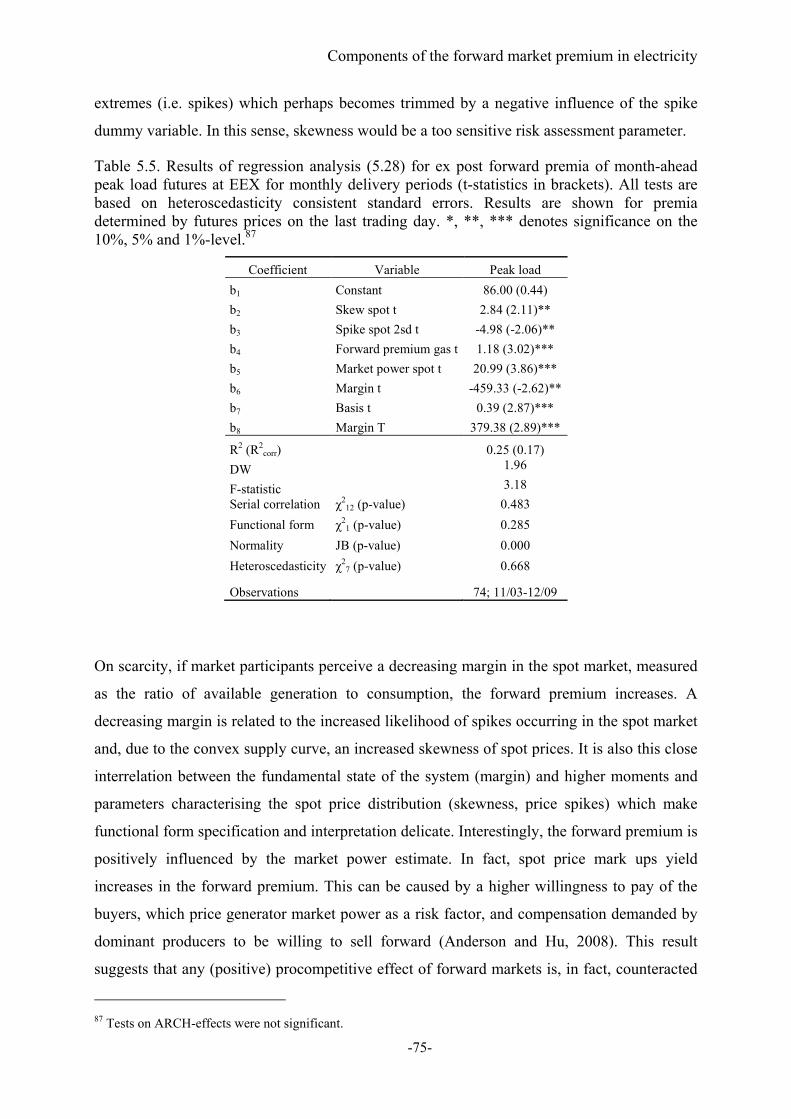
Components of the forward market premium in electricity
-75-
extremes (i.e. spikes) which perhaps becomes trimmed by a negative influence of the spike
dummy variable. In this sense, skewness would be a too sensitive risk assessment parameter.
Table 5.5. Results of regression analysis (5.28) for ex post forward premia of month-ahead peak load futures at EEX for monthly delivery periods (t-statistics in brackets). All tests are based on heteroscedasticity consistent standard errors. Results are shown for premia determined by futures prices on the last trading day. *, **, *** denotes significance on the 10%, 5% and 1%-level.87
On scarcity, if market participants perceive a decreasing margin in the spot market, measured
as the ratio of available generation to consumption, the forward premium increases. A
decreasing margin is related to the increased likelihood of spikes occurring in the spot market
and, due to the convex supply curve, an increased skewness of spot prices. It is also this close
interrelation between the fundamental state of the system (margin) and higher moments and
parameters characterising the spot price distribution (skewness, price spikes) which make
functional form specification and interpretation delicate. Interestingly, the forward premium is
positively influenced by the market power estimate. In fact, spot price mark ups yield
increases in the forward premium. This can be caused by a higher willingness to pay of the
buyers, which price generator market power as a risk factor, and compensation demanded by
dominant producers to be willing to sell forward (Anderson and Hu, 2008). This result
suggests that any (positive) procompetitive effect of forward markets is, in fact, counteracted
87 Tests on ARCH-effects were not significant.
Coefficient Variable Peak load
b1 Constant 86.00 (0.44)
b2 Skew spot t 2.84 (2.11)**
b3 Spike spot 2sd t -4.98 (-2.06)**
b4 Forward premium gas t 1.18 (3.02)***
b5 Market power spot t 20.99 (3.86)***
b6 Margin t -459.33 (-2.62)**
b7 Basis t 0.39 (2.87)***
b8 Margin T 379.38 (2.89)***
R2 (R2corr) 0.25 (0.17)
DW 1.96
F-statistic 3.18
Serial correlation χ212 (p-value) 0.483
Functional form χ21 (p-value) 0.285
Normality JB (p-value) 0.000
Heteroscedasticity χ27 (p-value) 0.668
Observations 74; 11/03-12/09
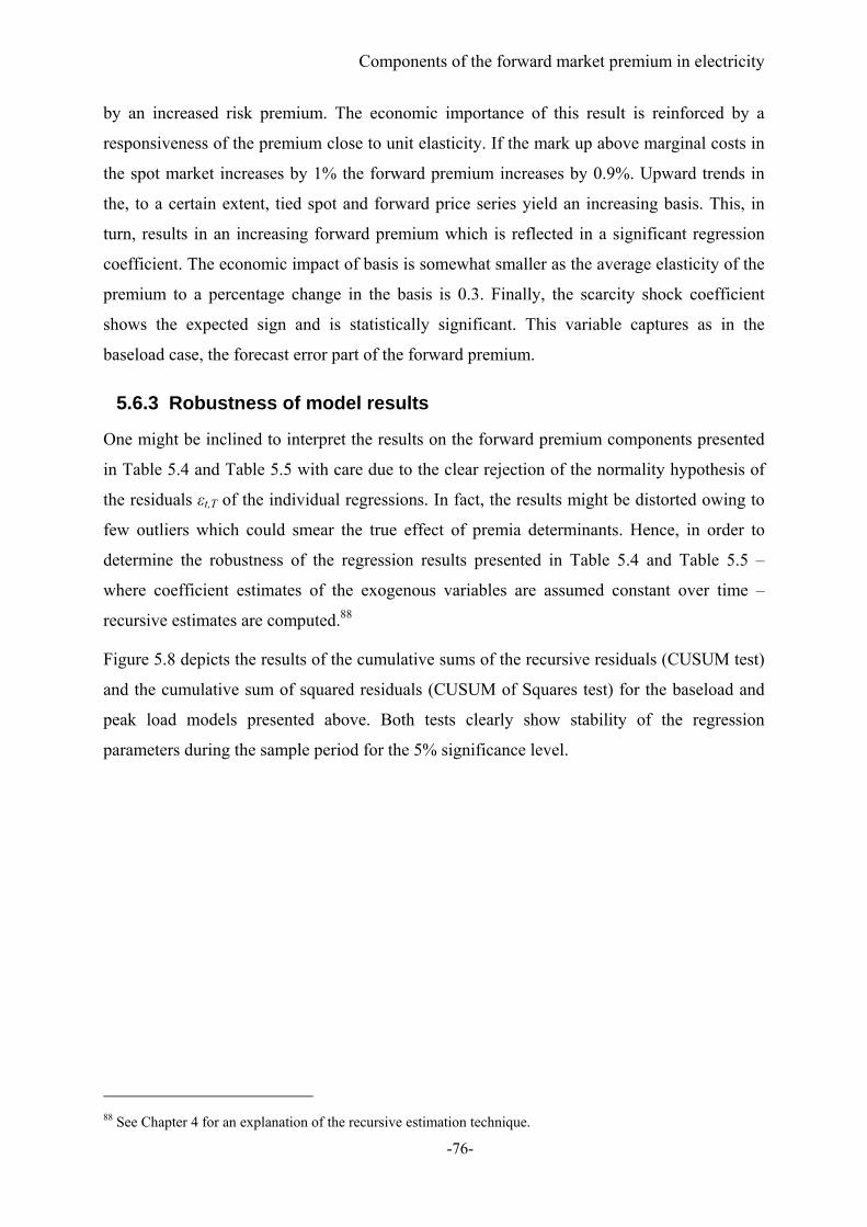
Components of the forward market premium in electricity
-76-
by an increased risk premium. The economic importance of this result is reinforced by a
responsiveness of the premium close to unit elasticity. If the mark up above marginal costs in
the spot market increases by 1% the forward premium increases by 0.9%. Upward trends in
the, to a certain extent, tied spot and forward price series yield an increasing basis. This, in
turn, results in an increasing forward premium which is reflected in a significant regression
coefficient. The economic impact of basis is somewhat smaller as the average elasticity of the
premium to a percentage change in the basis is 0.3. Finally, the scarcity shock coefficient
shows the expected sign and is statistically significant. This variable captures as in the
baseload case, the forecast error part of the forward premium.
5.6.3 Robustness of model results
One might be inclined to interpret the results on the forward premium components presented
in Table 5.4 and Table 5.5 with care due to the clear rejection of the normality hypothesis of
the residuals εt,T of the individual regressions. In fact, the results might be distorted owing to
few outliers which could smear the true effect of premia determinants. Hence, in order to
determine the robustness of the regression results presented in Table 5.4 and Table 5.5 –
where coefficient estimates of the exogenous variables are assumed constant over time –
recursive estimates are computed.88
Figure 5.8 depicts the results of the cumulative sums of the recursive residuals (CUSUM test)
and the cumulative sum of squared residuals (CUSUM of Squares test) for the baseload and
peak load models presented above. Both tests clearly show stability of the regression
parameters during the sample period for the 5% significance level.
88 See Chapter 4 for an explanation of the recursive estimation technique.
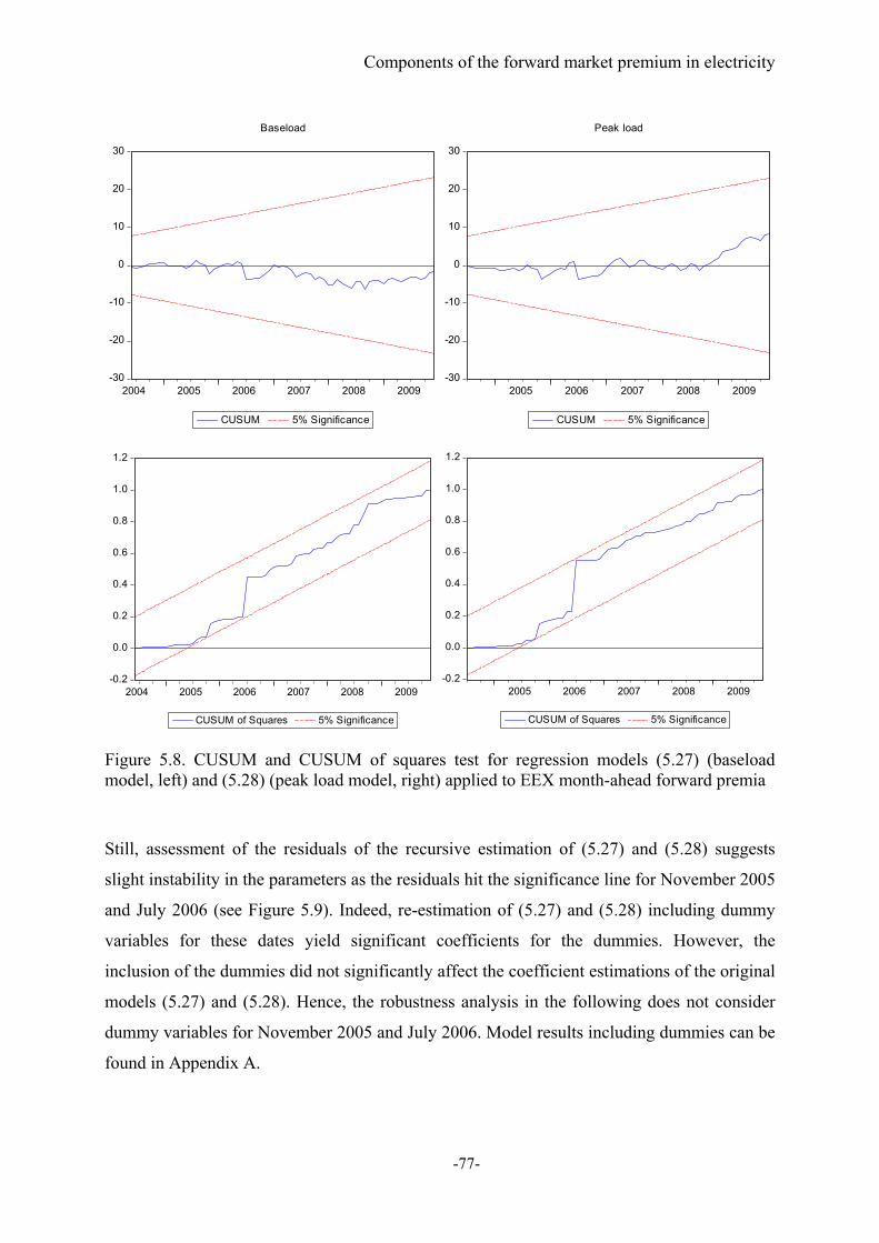
Components of the forward market premium in electricity
-77-
Figure 5.8. CUSUM and CUSUM of squares test for regression models (5.27) (baseload model, left) and (5.28) (peak load model, right) applied to EEX month-ahead forward premia
Still, assessment of the residuals of the recursive estimation of (5.27) and (5.28) suggests
slight instability in the parameters as the residuals hit the significance line for November 2005
and July 2006 (see Figure 5.9). Indeed, re-estimation of (5.27) and (5.28) including dummy
variables for these dates yield significant coefficients for the dummies. However, the
inclusion of the dummies did not significantly affect the coefficient estimations of the original
models (5.27) and (5.28). Hence, the robustness analysis in the following does not consider
dummy variables for November 2005 and July 2006. Model results including dummies can be
found in Appendix A.
-30
-20
-10
0
10
20
30
2004 2005 2006 2007 2008 2009
CUSUM 5% Significance
Baseload
-30
-20
-10
0
10
20
30
2005 2006 2007 2008 2009
CUSUM 5% Significance
Peak load
-0.2
0.0
0.2
0.4
0.6
0.8
1.0
1.2
2004 2005 2006 2007 2008 2009
CUSUM of Squares 5% Significance
-0.2
0.0
0.2
0.4
0.6
0.8
1.0
1.2
2005 2006 2007 2008 2009
CUSUM of Squares 5% Significance

Components of the forward market premium in electricity
-78-
Figure 5.9. Recursive residuals for regression models (6.26 – baseload model, left) and (6.27 – peak load model, right) applied to EEX month-ahead forward premia
Figure 5.10 presents graphs of the recursively estimated regression coefficients for the
baseload model (5.27). Clearly the parameters behave rather unstable at the beginning of the
sample period since the degrees of freedom of the model are low. However, as the sample size
increases, the estimates of the coefficients show a low variation which is an indicator of
parameter stability. Also the significance of the coefficients shows the expected trend
behaviour. Interestingly, the coefficient on the volatility in the oil market gets significant only
as of the year 2008. In fact, in this year the highest increases in the oil market history could be
observed – followed by a pronounced decrease. This, most likely, has caused the increased
awareness of market actors in the energy field to activities in the oil market and, in turn, the
increased importance of the oil market for the electricity market. Overall, the analysis of
recursive estimates for the baseload premium model has confirmed the robustness of the
results presented in Table 5.4.
-30
-20
-10
0
10
20
2004 2005 2006 2007 2008 2009
Recursive Residuals ± 2 S.E.
Baseload
-80
-60
-40
-20
0
20
40
2005 2006 2007 2008 2009
Recursive Residuals ± 2 S.E.
Peak load
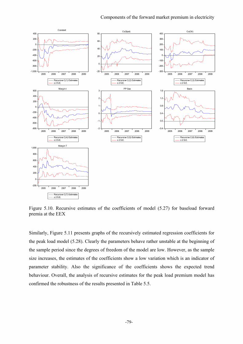
Components of the forward market premium in electricity
-79-
Figure 5.10. Recursive estimates of the coefficients of model (5.27) for baseload forward premia at the EEX
Similarly, Figure 5.11 presents graphs of the recursively estimated regression coefficients for
the peak load model (5.28). Clearly the parameters behave rather unstable at the beginning of
the sample period since the degrees of freedom of the model are low. However, as the sample
size increases, the estimates of the coefficients show a low variation which is an indicator of
parameter stability. Also the significance of the coefficients shows the expected trend
behaviour. Overall, the analysis of recursive estimates for the peak load premium model has
confirmed the robustness of the results presented in Table 5.5.
-1,000
-800
-600
-400
-200
0
200
400
2005 2006 2007 2008 2009
Recursive C(1) Estimates± 2 S.E.
-20
0
20
40
60
80
2005 2006 2007 2008 2009
Recursive C(2) Estimates± 2 S.E.
-300
-200
-100
0
100
200
300
400
2005 2006 2007 2008 2009
Recursive C(3) Estimates± 2 S.E.
-800
-600
-400
-200
0
200
400
600
2005 2006 2007 2008 2009
Recursive C(4) Estimates± 2 S.E.
-2
-1
0
1
2
3
2005 2006 2007 2008 2009
Recursive C(5) Estimates± 2 S.E.
-0.4
0.0
0.4
0.8
1.2
1.6
2005 2006 2007 2008 2009
Recursive C(6) Estimates± 2 S.E.
-200
0
200
400
600
800
1,000
2005 2006 2007 2008 2009
Recursive C(7) Estimates± 2 S.E.
ConstantCv(Spot) Cv(Oil)
Margin t FP Gas Basis
Margin T
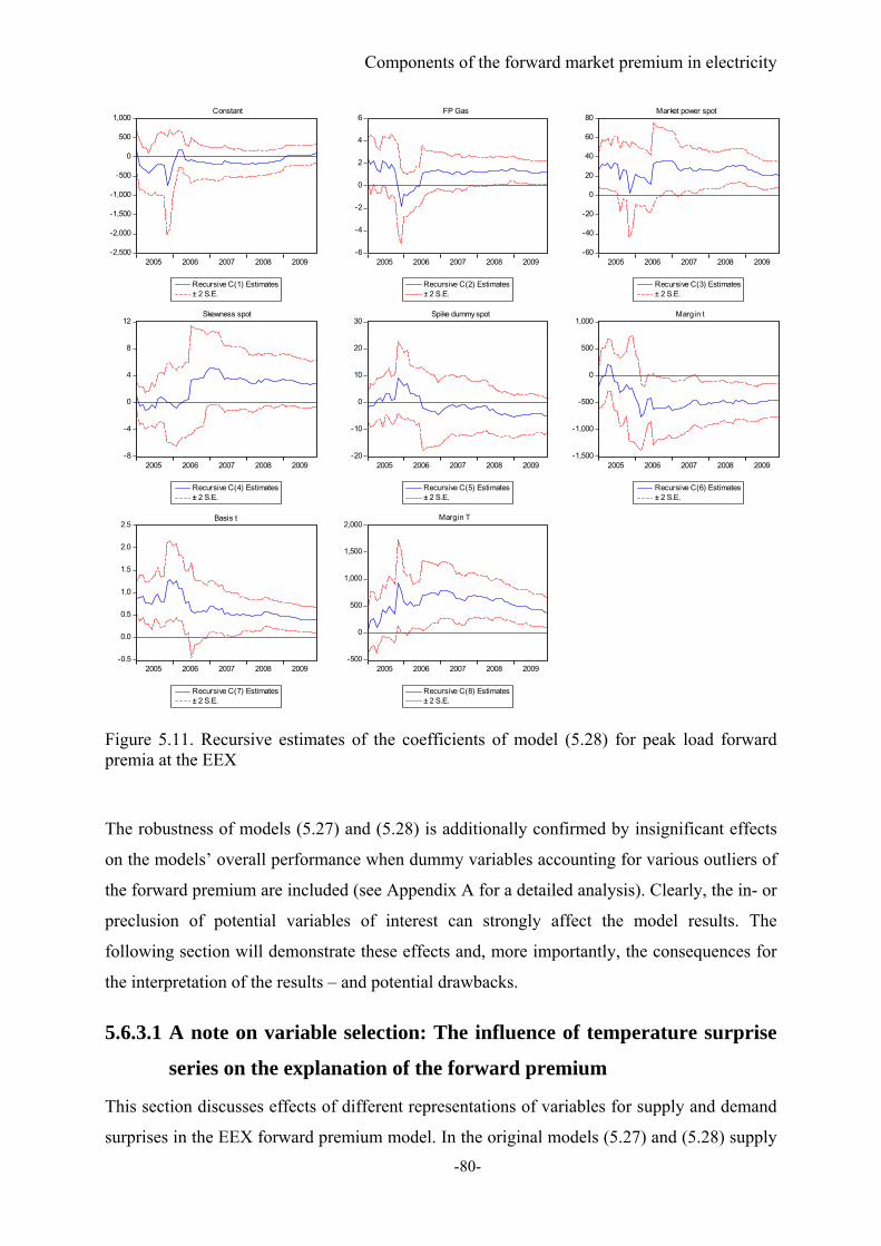
Components of the forward market premium in electricity
-80-
Figure 5.11. Recursive estimates of the coefficients of model (5.28) for peak load forward premia at the EEX
The robustness of models (5.27) and (5.28) is additionally confirmed by insignificant effects
on the models’ overall performance when dummy variables accounting for various outliers of
the forward premium are included (see Appendix A for a detailed analysis). Clearly, the in- or
preclusion of potential variables of interest can strongly affect the model results. The
following section will demonstrate these effects and, more importantly, the consequences for
the interpretation of the results – and potential drawbacks.
5.6.3.1 A note on variable selection: The influence of temperature surprise
series on the explanation of the forward premium
This section discusses effects of different representations of variables for supply and demand
surprises in the EEX forward premium model. In the original models (5.27) and (5.28) supply
-2,500
-2,000
-1,500
-1,000
-500
0
500
1,000
2005 2006 2007 2008 2009
Recursive C(1) Estimates± 2 S.E.
-6
-4
-2
0
2
4
6
2005 2006 2007 2008 2009
Recursive C(2) Estimates± 2 S.E.
-60
-40
-20
0
20
40
60
80
2005 2006 2007 2008 2009
Recursive C(3) Estimates± 2 S.E.
-8
-4
0
4
8
12
2005 2006 2007 2008 2009
Recursive C(4) Estimates± 2 S.E.
-20
-10
0
10
20
30
2005 2006 2007 2008 2009
Recursive C(5) Estimates± 2 S.E.
-1,500
-1,000
-500
0
500
1,000
2005 2006 2007 2008 2009
Recursive C(6) Estimates± 2 S.E.
-0.5
0.0
0.5
1.0
1.5
2.0
2.5
2005 2006 2007 2008 2009
Recursive C(7) Estimates± 2 S.E.
-500
0
500
1,000
1,500
2,000
2005 2006 2007 2008 2009
Recursive C(8) Estimates± 2 S.E.
Constant FP Gas Market power spot
Skewness spot Spike dummy spot Margin t
Basis t Margin T

Components of the forward market premium in electricity
-81-
and demand shocks are captured by one common margin shock variable in order to avoid
long-term trend effects of a separate consumption and generation representation. The aim of
this section is to point out the importance of a careful parameter selection in an empirical
model and to show consequences for the results of different model specifications – in terms of
both statistical as well as fundamental properties.
Demand surprises
By using average daily temperature data from the University of Dayton
(http://www.engr.udayton.edu/weather/), available from January 1995, it is possible to
construct monthly temperature time series for several cities (mainly the capitals) in the
relevant regional electricity market. The monthly temperature series are highly correlated
(correlation coefficient > 0.96). Hence, the core regional Western European market (Austria,
France, Germany, and Switzerland) and corresponding average temperature series are used for
the demand surprise analysis.
Using monthly temperature series allows the calculation of a surprise variable which
measures the difference between the actual average temperature in the delivery month of the
futures contract and the historic average in the specific month. Figure 5.12 shows the
temperature surprises from October 2003 to January 2010.
Figure 5.12. Temperature surprises (absolute values: black line and left scale; relative values: grey line and right scale) in the delivery months of the forward contracts computed as differences to the historic long term values. Source: http://www.engr.udayton.edu/weather/, own calculations
‐2,0
‐1,5
‐1,0
‐0,5
0,0
0,5
1,0
1,5
2,0
2,5
3,0
‐5
‐4
‐3
‐2
‐1
0
1
2
3
4
5
Okt.03
Mär.04
Aug.04
Jän.05
Jun.05
Nov.05
Apr.06
Sep.06
Feb.07
Jul.07
Dez.07
Mai.08
Okt.08
Mär.09
Aug.09
Jän.10
[‐]
[°C]
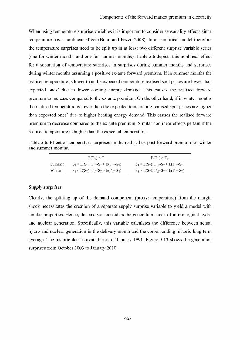
Components of the forward market premium in electricity
-82-
When using temperature surprise variables it is important to consider seasonality effects since
temperature has a nonlinear effect (Bunn and Fezzi, 2008). In an empirical model therefore
the temperature surprises need to be split up in at least two different surprise variable series
(one for winter months and one for summer months). Table 5.6 depicts this nonlinear effect
for a separation of temperature surprises in surprises during summer months and surprises
during winter months assuming a positive ex-ante forward premium. If in summer months the
realised temperature is lower than the expected temperature realised spot prices are lower than
expected ones’ due to lower cooling energy demand. This causes the realised forward
premium to increase compared to the ex ante premium. On the other hand, if in winter months
the realised temperature is lower than the expected temperature realised spot prices are higher
than expected ones’ due to higher heating energy demand. This causes the realised forward
premium to decrease compared to the ex ante premium. Similar nonlinear effects pertain if the
realised temperature is higher than the expected temperature.
Table 5.6. Effect of temperature surprises on the realised ex post forward premium for winter and summer months.
E(TT) < TT E(TT) > TT
Summer ST > E(ST): Ft,T-ST < E(Ft,T-ST) ST < E(ST): Ft,T-ST > E(Ft,T-ST)
Winter ST < E(ST): Ft,T-ST > E(Ft,T-ST) ST > E(ST): Ft,T-ST < E(Ft,T-ST)
Supply surprises
Clearly, the splitting up of the demand component (proxy: temperature) from the margin
shock necessitates the creation of a separate supply surprise variable to yield a model with
similar properties. Hence, this analysis considers the generation shock of inframarginal hydro
and nuclear generation. Specifically, this variable calculates the difference between actual
hydro and nuclear generation in the delivery month and the corresponding historic long term
average. The historic data is available as of January 1991. Figure 5.13 shows the generation
surprises from October 2003 to January 2010.
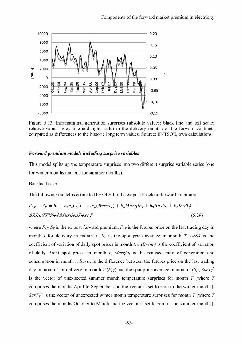
Components of the forward market premium in electricity
-83-
Figure 5.13. Inframarginal generation surprises (absolute values: black line and left scale; relative values: grey line and right scale) in the delivery months of the forward contracts computed as differences to the historic long term values. Source: ENTSOE, own calculations
Forward premium models including surprise variables
This model splits up the temperature surprises into two different surprise variable series (one
for winter months and one for summer months).
Baseload case
The following model is estimated by OLS for the ex post baseload forward premium:
,
7 8 , (5.29)
where Ft,T-ST is the ex post forward premium, Ft,T is the futures price on the last trading day in
month t for delivery in month T, ST is the spot price average in month T, cv(St) is the
coefficient of variation of daily spot prices in month t, cv(Brentt) is the coefficient of variation
of daily Brent spot prices in month t, Margint is the realised ratio of generation and
consumption in month t, Basist is the difference between the futures price on the last trading
day in month t for delivery in month T (Ft,T) and the spot price average in month t (St), SurTTS
is the vector of unexpected summer month temperature surprises for month T (where T
comprises the months April to September and the vector is set to zero in the winter months),
SurTTW is the vector of unexpected winter month temperature surprises for month T (where T
comprises the months October to March and the vector is set to zero in the summer months),
‐0,15
‐0,10
‐0,05
0,00
0,05
0,10
0,15
0,20
‐8000
‐6000
‐4000
‐2000
0
2000
4000
6000
8000
10000
Okt.03
Mär.04
Aug.04
Jän.05
Jun.05
Nov.05
Apr.06
Sep.06
Feb.07
Jul.07
Dez.07
Mai.08
Okt.08
Mär.09
Aug.09
[‐]
[GWh]
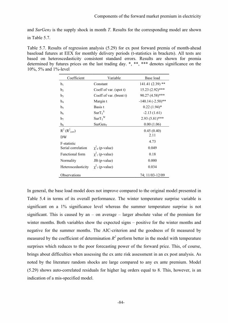
Components of the forward market premium in electricity
-84-
and SurGenT is the supply shock in month T. Results for the corresponding model are shown
in Table 5.7.
Table 5.7. Results of regression analysis (5.29) for ex post forward premia of month-ahead baseload futures at EEX for monthly delivery periods (t-statistics in brackets). All tests are based on heteroscedasticity consistent standard errors. Results are shown for premia determined by futures prices on the last trading day. *, **, *** denotes significance on the 10%, 5% and 1%-level
Coefficient Variable Base load
b1 Constant 141.41 (2.39) **
b2 Coeff of var. (spot t) 15.23 (2.92)***
b3 Coeff of var. (brent t) 90.27 (4.58)***
b4 Margin t -140.14 (-2.50)**
b5 Basis t 0.22 (1.94)*
b6 SurTTS -2.13 (1.61)
b7 SurTTW 2.93 (5.81)***
b8 SurGenT 0.00 (1.06)
R2 (R2corr) 0.45 (0.40)
DW 2.11
F-statistic 4.73
Serial correlation χ28 (p-value) 0.049
Functional form χ21 (p-value) 0.18
Normality JB (p-value) 0.000
Heteroscedasticity χ27 (p-value) 0.034
Observations 74; 11/03-12/09
In general, the base load model does not improve compared to the original model presented in
Table 5.4 in terms of its overall performance. The winter temperature surprise variable is
significant on a 1% significance level whereas the summer temperature surprise is not
significant. This is caused by an – on average – larger absolute value of the premium for
winter months. Both variables show the expected signs – positive for the winter months and
negative for the summer months. The AIC-criterion and the goodness of fit measured by
measured by the coefficient of determination R2 perform better in the model with temperature
surprises which reduces to the poor forecasting power of the forward price. This, of course,
brings about difficulties when assessing the ex ante risk assessment in an ex post analysis. As
noted by the literature random shocks are large compared to any ex ante premium. Model
(5.29) shows auto-correlated residuals for higher lag orders equal to 8. This, however, is an
indication of a mis-specified model.

Components of the forward market premium in electricity
-85-
Peak load case
The following model is estimated by OLS for the ex post peak load forward premium:
, . ,
, (5.30)
where Ft,T-ST is the ex post forward premium, Ft,T is the peak load futures price on the last
trading day in month t for delivery during peak hours in month T, ST is the peak load spot
price average in month T, Skew(St) is the skewness of daily spot prices in month t, Spike2.5sd t
is the count of spikes outside of 2.5 standard deviations of the mean spot price in month t,
FPGas t-1,t is the realised gas forward premium of a month ahead futures for month t, Spot
market powert is the ratio of the spot price in month t and the fundamental marginal cost
estimate for month t, Margint is the ratio of regional generation and demand in month t, Basist
is the difference between the futures price on the last trading day in month t for delivery in
month T (Ft,T) and the spot price average in month t (St), SurTTS is the vector of unexpected
summer month temperature surprises for month T (where T comprises the months April to
September and the vector is set to zero in the winter months), SurTTW is the vector of
unexpected winter month temperature surprises for month T (where T comprises the months
October to March and the vector is set to zero in the summer months), and MarginT is the
margin shock in month T. Results for the corresponding model are shown in Table 5.8.
In general, the peak load model improves compared to the original model presented in Table
5.5 in terms of its overall performance. The winter temperature surprise variable is significant
on a 1% significance level whereas the summer temperature surprise is not significant. This is
caused by an – on average – larger absolute value of the premium for winter months. Both
variables show the expected signs – positive for the winter months and negative for the
summer months. The supply side surprise variable is not statistically significant. The
goodness of fit measured by the coefficient of determination R2 and the AIC-criterion improve
which reduces to the poor forecasting power of the forward price. Still, the performance of the
model (5.30) is not conclusive. Much of the variation in the forward premium is captured by a
significant constant term. This, however, is not a satisfying result when analysing the time-
varying properties of the forward premium.
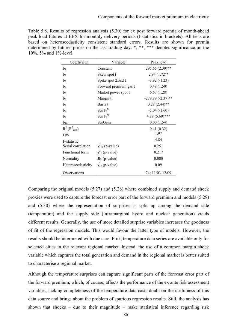
Components of the forward market premium in electricity
-86-
Table 5.8. Results of regression analysis (5.30) for ex post forward premia of month-ahead peak load futures at EEX for monthly delivery periods (t-statistics in brackets). All tests are based on heteroscedasticity consistent standard errors. Results are shown for premia determined by futures prices on the last trading day. *, **, *** denotes significance on the 10%, 5% and 1%-level
Coefficient Variable Peak load
b1 Constant 295.65 (2.39)**
b2 Skew spot t 2.94 (1.72)*
b3 Spike spot 2.5sd t -3.92 (-1.23)
b4 Forward premium gas t 0.48 (1.50)
b5 Market power spot t 6.67 (1.28)
b6 Margin t -279.89 (-2.37)**
b7 Basis t 0.28 (2.44)**
b8 SurTTS -5.04 (-1.60)
b9 SurTTW 4.88 (5.69)***
b10 SurGenT 0.00 (1.54)
R2 (R2corr) 0.41 (0.32)
DW 1.97
F-statistic 4.84
Serial correlation χ212 (p-value) 0.251
Functional form χ21 (p-value) 0.217
Normality JB (p-value) 0.000
Heteroscedasticity χ29 (p-value) 0.09
Observations 74; 11/03-12/09
Comparing the original models (5.27) and (5.28) where combined supply and demand shock
proxies were used to capture the forecast error part of the forward premium and models (5.29)
and (5.30) where the representation of surprises is split up among the demand side
(temperature) and the supply side (inframarginal hydro and nuclear generation) yields
different results. Generally, the use of more detailed surprise variables increases the goodness
of fit of the regression models. This would favour the latter type of models. However, the
results should be interpreted with due care. First, temperature data series are available only for
selected cities in the relevant regional market. Instead, the use of a common margin shock
variable which captures the total generation and demand in the regional market is better suited
to characterise a regional market.
Although the temperature surprises can capture significant parts of the forecast error part of
the forward premium, which, of course, affects the performance of the ex ante risk assessment
variables, lacking completeness of the temperature data casts doubt on the usefulness of this
data source and brings about the problem of spurious regression results. Still, the analysis has
shown that shocks – due to their magnitude – make statistical inference regarding risk
Components of the forward market premium in electricity
-87-
assessment delicate. However, due to the nature of the temperature data, this result may be the
cause of a pretended accuracy of the temperature data. The fundamental (aggregated) margin
variable presents itself to be a more precise representation of shocks occurring in the regional
market.
5.7 Conclusions
This chapter has introduced a multifactor analysis of electricity forward premia determinants
to give insights into some important propositions on the electricity forward premium. In
general several significant new effects have been shown:
The ex post nature of the analysis was controlled for by including a margin shock
variable in the regressions, and this was indeed significant in both the peak and
baseload monthly ex post risk premia.
As a derived commodity, electricity translates a substantial amount of the underlying
fuel’s market price of risk (i.e. the peak forward premium is in fact determined partly
due to the gas market).
As part of the energy commodity trading bundle, oil market sentiment spills over, in
that increased oil price volatility increases the forward premium.
Market concentration appears to have a double influence on power prices – in addition
to its potential effect on spot prices, it increases the forward premium. It seems
therefore that whilst the theoretical effect of forward contracting may be to make the
spot market more competitive, generators are able to compensate for this through a
higher forward premium.89
The effects of scarcity (reserve margin), spot volatility and skewness were significant
and consistent with propositions on the positive effects of market risk aversion.
Overall, the forward premium in electricity is a rather complex function of fundamental,
behavioural, dynamic, market conduct and shock components. It is clearly an
oversimplification in practice to analyse it only in terms of the stochastic properties of the
89 The theoretical model of Allaz and Vila (1993) indicated an increase in physical supply of 20% compared to the no contract case, and in a similar way Green (1999) estimates, in a numerical example, price decreases of 25% when comparing fully contracted to uncontracted firms. The extensive analyses by Bushnell (2007, et. al., 2008) suggests price decreases of around 50% when firms’ contract positions are considered against a theoretical counterfactual. This contrasts with actual empirical studies reporting significant positive forward premia: Longstaff and Wang (2004) show for the PJM day ahead market premia up to 14%. Botterud et al. (2009) report for the Nord Pool market baseload premia from 1.3 to 4.4% for one week to six weeks ahead. Similarly, Redl et al. (2009) determine Nord Pool baseload premia of 8% for month-ahead contracts and EEX month-ahead premia of 9% for baseload and 13% for peak load.
Components of the forward market premium in electricity
-88-
spot prices (variance and skewness). Only part of the risk can be attributed to the electricity
sector per se, but in that, risk aversion to scarcity, volatility and extreme events, as well as
behavioural adaptation and oil sentiment spillovers characterises agent behaviour.
Furthermore, market concentration appears to translate market power effects into the risk
premium, which may have important market monitoring implications since forward markets
have, so far, been considered to be procompetitive.90 Policy makers and regulators seek to
increase consumer welfare. In the context of electricity markets this is associated with
measures aiming to reduce the forward premium. The reserve margin plays therefore a crucial
role since increased scarcity increases spot prices (which is amplified in the case of
concentrated markets) and, moreover, also the forward premium. Hence, consumers take a
“double hit” if the margin reduces, and if this is due to strategic withholding, then it is an
important anti-trust concern. In general, some of the insights presented here suggest that
forward premia should be considered key elements of a transaction cost view of market
efficiency in power trading.
Finally, the analysis purposely relied on variables which are observable for the market actors
on the forward trading day. As some of the fundamental market data is publicly available only
on a monthly basis, the definition of the forward premium on the last trading day is
particularly attractive for analysis. A more thorough investigation of the dynamic
interrelations between current spot and forward prices (and premia) would, however, benefit
from the higher granularity of daily representations or even higher frequency impact studies
of news on forward prices.
90 See Anderson and Hu (2008) for a similar argument arising from a theoretical equilibrium model.
Conclusions and Outlook
-89-
6 Conclusions and Outlook
This thesis contributed to the literature analysing the functioning of deregulated wholesale
electricity markets. Specifically, it focused on the empirical assessment of major European
long-term futures and forward markets. Wholesale market participants are faced with a
multitude of uncertainties and risks. Long-term markets are particularly attractive from a risk
management point of view as they allow for hedging price risks. High trading volumes on
these markets, eventually exceeding actual physical demand, reflect their importance.
High trading volumes and, correspondingly, high market liquidity are generally considered as
indications of mature and well-functioning markets. Yet it is crucial to gain deeper insight
into the price formation process – not at least because of the special characteristics of the
physical commodity electricity, associated consequences for the market structure, and its
importance for the overall economy. These insights enable an efficient and effective design of
the markets and its regulatory and legislative provisions.
The analyses carried out contribute to an assessment of the deregulation exercise of the
European power sector. Firstly, the main drivers of year-ahead futures prices at the two
analysed major European power markets (the EEX and Nord Pool power exchanges) were
analysed. It was followed by a high-frequency analysis of the interaction between spot and
forward prices of different maturities and their drivers. Finally, the price of risk inherent in the
long-term markets was studied by a multifactor analysis of month-ahead forward premia and
their corresponding determinants. These analyses have revealed several new effects:
Year-ahead futures prices are both influenced by expectations of generation costs of price
setting power plant technologies and current spot market prices. This pricing mechanism
could be revealed for both of the two analysed markets. In fact, the results suggest that the
pricing of futures is a complex function of rational91 and behavioural components.
The results of the high-frequency analysis of the daily electricity price system support this
finding. The price system consists of daily spot and forward prices of various maturities. First,
fundamental supply and demand variables effect the system of electricity prices. Second,
electricity spot prices influence electricity futures prices and vice versa. These results appear
particularly surprising given the non-storability of electricity and are counter to the
implications of a rational pricing model of non-storable commodities. In turn, they cast doubt
91 In the neo-classical sense.
Conclusions and Outlook
-90-
on the predictive power of forward prices and on market efficiency. Additionally, the tie in
storable fuels implies the corresponding cost of carry also effecting the non-storable
commodity electricity. Consequently, this complicates the price formation. Furthermore, the
risk assessment of market participants gets affected increasing the cost of hedging spot price
uncertainty.
Specifically, the effects of compound forward pricing on the futures prices’ inherent price of
risk were revealed by a multifactor analysis of realised month-ahead forward premia. The
premia are a complex function of fundamental, behavioural, market structure, dynamic and
external shock components. These premia determinants are partly in line with theories of risk
aversion of rational market participants. The action of spill over and market power effects,
however, reveals unexpected significant transaction costs associated with power trading.
What are the implications for the performance of electricity wholesale markets? Firstly, the
conducted analyses give insights into the structure of the market participants. For example, as
of January 2011 about 150 organisations, including all major (investment) banks, were
registered for trading in the EEX’s power derivatives market92. On average a subset of about
50 are actively participating.93 The performed analyses suggest that futures market results are
largely determined by market actors with a physical position (i.e. generators, retailers and
large consumers). This is indicated by the magnitude of realised forward premia in the order
of 10% on a monthly basis. The premium would represent the willingness to pay for risk
reduction if systematic forecast errors were neglected (i.e. market participants forming
rational expectations). Forward premia are also affected by external shocks. Still, it is possible
to contend that premia on the short-end of the forward curve are largely determined by risk
averse buyers because there are significant trend effects in the time to maturity behaviour of
the premia.
Sufficient short selling of futures contracts of “outside” speculators, that is, market actors
without a physical position, would bring down these premia to a level determined by
transaction costs.94 Yet increased trading activities in markets can cause price volatility to
92 http://www.eex.com/en/EEX/Participants 93 http://www.eex.com/en/Transparency 94 Speculative positions in derivative markets are taken in response to price differences between futures and consecutive spot prices. “Speculators” acting in financial markets do not have delivery obligations in physical markets. It is worthwhile to point out that every trade in financial contracts markets, i.e. also risk management activities of participants with physical positions, is partly determined by a speculative position. See chapter 2.3.2 for details.
Conclusions and Outlook
-91-
increase.95 Forward premia should decrease in absolute terms if the number of speculative
trades grows. It might, however, have implications for the price of risk due to an increased
short-term volatility. These implications are not clear cut in an electricity price system
characterised by repercussions among the price series. They suggest further investigation.
Speculative trading activities in energy commodity markets have caused a lively public debate
about its effects on price levels, especially since prices in the crude oil market rose to
unprecedented highs in 2008. Sole speculative trading can be ruled out to be responsible for
the electricity futures price formation for reasons outlined above. Still, prices on long-term
markets are driven by expectations and corresponding trades bring about an equilibrium
market price. In essence, these trades on derivative markets are zero sum games.96 Hence, if
markets “don’t get it right” it is also an issue of market participants’ expectations.
The analysis in this thesis has revealed that the futures price formation and, correspondingly,
the expectation formation of the market participants are a compound mix of rational and
several behavioural components. As market equilibrium is linked to equilibrium in
expectations the existence of behavioural effects applies for all groups of market participants.
Future research could build a formal model of different groups of market actors detailing
psychological biases. This could shed light on the specific short and long positions taken in
the forward markets. Moreover, this would allow testing for expectations induced trend
(herding) effects.
Futures prices are affected by behavioural pricing components and a – due to changing
degrees of risk aversion – time-varying market price of risk. In combination with shock (i.e.
uncertainty) induced errors these influences yield, in terms of forecasting power, a biased
futures price. On the month-ahead level this adds up to forward prices being on average in the
order of 10% above subsequent spot prices. This unfolds market monitoring issues. The
analyses suggest that market power effects of concentrated supply structures spill over to
forward premia due to a risk averse demand. Lacking transparency on the positions entered by
market actors not only makes empirical analysis an elusive task but also determines
95 In fact, there is theoretical and empirical evidence that derivative markets in particular are characterised by a positive correlation between traded volume (being a proxy for new information) and price volatility. For details see Fontana et al. (2007) and the references therein. 96 More specifically, each trade is a zero sum game on a microeconomic level. Clearly, well functioning forward markets have a positive value on a macroeconomic level. See chapter 2.2 for details.
Conclusions and Outlook
-92-
information asymmetries.97 Information asymmetry though renders an inefficient resource
allocation on markets (Stiglitz, 2001).
The spill over of market power effects into the forward premium, in turn, has essential
monitoring implications since forward markets have, so far, been considered to be
procompetitive. Analyses concerning market power effects in electricity markets focus
typically on spot markets only. Whereas these studies do confirm the crucial role of excess
supply capacities and of strategic withholding on spot market results the impact of margin and
mark ups on risk aversion is not considered.
Publications of the USA based Commodity Futures Trading Commission (CFTC) list long
and short open interests of different types of traders.98 If such market transparency
programmes were implemented in the European electricity futures markets this would
decrease asymmetries and increase the data base for new descriptive analysis and new
theories on decision making of market participants.99 In fact, publication on aggregated trader
category levels would take into account the trade-off between reducing asymmetries and
releasing sensitive business related information.
The analyses in this thesis have relied on aggregated market data – basically settlement prices
of different commodities and fundamental supply and demand quantities. The insights could
be enlarged by the inclusion of data related to the positions taken, at least on aggregate, by
hedgers and speculators and market concentrations. The robustness of the results could be
increased by assessing additional forward contract maturities and taking into account higher
granularities of daily or intra-daily price time series. Still, this would necessitate far higher
transparency levels.
New empirical insights can frame new theories of decision making under risk. This thesis
provided empirical insights into the price formation in electricity futures markets. They
suggest expanding existing equilibrium models considering oligopolistic market
environments, psychologically based behavioural concepts and different information levels.
97 This applies both for organised marketplaces (i.e. power exchanges) and bilateral OTC trades. 98 Commitment of Traders reports available at http://www.cftc.gov/MarketReports/CommitmentsofTraders/index.htm 99 Indeed, European Commission (2010) proposes draft rules on regulative oversight of trading in wholesale power markets. This proposal includes data collection on transactions and corresponding orders.
References
-93-
References
Allaz, B., 1992. Oligopoly, uncertainty and strategic forward transactions. International
Journal of Industrial Organization 10, 297-308.
Allaz, B., Vila, J.L., 1993. Cournot Competition, Forward Markets and Efficiency. Journal of
Economic Theory 59, 1-16.
Anderson, R.W., Danthine, J.P., 1981. Cross Hedging. Journal of Political Economy 89(6),
1182-1196.
Anderson, E.J., Hu, X., 2008. Forward contracts and market power in an electricity market.
International Journal of Industrial Organization 26, 679-694.
Bekiros, S.D., Diks, C.G.H., 2008. The relationship between crude oil spot and futures prices:
Cointegration, linear and nonlinear causality. Energy Economics 30, 2673-2685.
Benth, F.E., Cartea, A., Kiesel, R., 2008. Pricing forward contracts in power markets by the
certainty equivalence principle: Explaining the sign of the market risk premium. Journal of
Banking & Finance 32, 2006-2021.
Benth, F.E., Koekebakker, S., 2008. Stochastic modeling of financial electricity contracts.
Energy Economics 30(3), 1116-1157.
Benth, F.E., Meyer-Brandis, T., 2009. The information premium for non-storable
commodities. The Journal of Energy Markets 2(3), 111-140.
Bessembinder, H., 1992. Systematic Risk, Hedging Pressure, and Risk Premiums in Futures
Markets. The Review of Financial Studies 5(4), 637-667.
Bessembinder, H., Lemmon, M.L., 2002. Equilibrium Pricing and Optimal Hedging in
Electricity Forward Markets. The Journal of Finance 57(3), 1347-1382.
Bierbauer, M., Menn, C., Rachev, S.T., Trück, S., 2007. Spot and derivative pricing in the
EEX power market. Journal of Banking & Finance 31, 3462-3485.
Botterud, A., Bhattacharyya, A., Ilic, M., 2002. Futures and spot prices – an analysis of the
Scandinavian electricity market. Working Paper.
Botterud, A., Kristiansen, T., Ilic, M., 2009. The relationship between spot and futures prices
in the Nord Pool electricity market. Energy Economics, In Press,
doi:10.1016/j.eneco.2009.11.009.
References
-94-
Borenstein, S., Bushnell, J., Knittel, C.R., Wolfram, C., 2008. Inefficiencies and market
power in financial arbitrage: A study of California’s electricity markets. The Journal of
Industrial Economics, LVI(2), 347-378.
Bowden, N., Payne, J.E., 2008. Short Term Forecasting of Electricity Prices for MISO Hubs:
Evidence from ARIMA-EGARCH Models. Energy Economics 30(6), 3186-3197.
Bunn, D.W., 2004. Modelling Prices in Competitive Electricity Markets. Wiley.
Bunn, D.W., 2006. Risk and electricity price dynamics. Platts.com News Feature.
Bunn D., Fezzi C., 2008. A vector error correction model of the interactions among gas,
electricity and carbon prices: an application to the cases of Germany and United Kingdom, in
(Editor: F. Gulli): Markets for carbon and power pricing in Europe: theoretical issues and
empirical analyses, Edward Elgar Publishing, pp. 145-159.
Bunn, D.W., Gianfreda, A., 2009. Integration and shock transmissions across European
electricity forward markets. Energy Economics 32(2), 278-291.
Bunn, D.W., Karakatsani, N., 2003. Forecasting Electricity Prices. London Business School,
London.
Burger, M., Klar, B., Müller, A., Schindlmayr, G., 2004. A spot market model for pricing
derivatives in electricity markets. Quantitative Finance 4(1), 109-122.
Bushnell, J., 2007. Oligopoly equilibria in electricity contract markets. Journal of Regulatory
Economics 32, 225-245.
Bushnell, J., Mansur, E.T., and Saravia, C., 2008. Vertical Arrangements, Market Structure
and Competition: An Analysis of Restructured US Electricity Markets. American Economic
Review, 98 (1) 237-266.
Christensen, B.J., Jensen, T.E., Molgaard, R., 2007. Market Power in Power Markets:
Evidence from Forward Prices of Electricity. CREATES Research Paper 2007-30.
www.creates.au.dk
Clewlow, L., Strickland, C., 2000. Energy Derivatives: Pricing and Risk Management.
Lacima Publications, London.
Cox, J., C., Ingersoll, J., Ross, S.A., 1981. The relation between forward prices and futures
prices. Journal of Financial Economics 9(4), 321-346.
References
-95-
Danthine, J.P., 1978. Information, Futures Prices, and Stabilizing Speculation. Journal of
Economic Theory 17, 79-98.
Daskalakis, G., Markellos, R., N., 2009. Are electricity risk premia affected by emission
allowance prices? Evidence from the EEX, Nord Pool and Powernext. Energy Policy (37).
2594-2604.
Diko, P., Lawford, S., Limpens, V., 2006. Risk Premia in Electricity Forward Markets.
Studies in Nonlinear Dynamics & Econometrics 10(3), Article 7.
Douglas, S., Popova, J., 2008. Storage and the electricity forward premium. Energy
Economics 30(4), 1712-1727.
Engle, R., Granger, C., 1987. Cointegration and Error Correction Representation, Estimation
and Testing. Econometrica 55, 251-276.
European Commission. 1996. Services of general interest in Europe. Official Journal of the
European Communities, 96/C 281/03.
European Commission, 1997. Directive 96/92/EC of the European Parliament and of the
Council concerning common rules for the internal market in electricity. L027, Brussels.
European Commission, 2003. Directive 2003/54/EC of the European Parliament and of the
Council concerning common rules for the internal market in electricity and repealing
Directive 96/92/EC. L176, Brussels.
European Commission, 2005. Report on progress in creating the internal gas and electricity
market. Communication from the Commission to the Council and the European Parliament,
COM(2005) 568 final, Brussels.
European Commission, 2007a. Proposal for a Directive of the European Parliament and of the
Council amending Directive 2003/54/EC concerning common rules for the internal market in
electricity COM(2007) 528 final. Brussels: Commission of the European Communities.
European Commission, 2007b. DG Competition report on energy sector inquiry. SEC(2006)
1724, Brussels.
European Commission, 2008. Accompanying document to the Report on Progress in Creating
the Internal Gas and Electricity Market, COM(2008) 192 final, Brussels.
European Commission, 2009. Directive 2009/72/EC of the European Parliament and of the
Council concerning common rules for the internal market in electricity and repealing
Directive 2003/54/EC. L211, Brussels.
References
-96-
European Commission, 2010. Proposal for a Regulation of the European Parliament and of
the Council on energy market integrity and transparency. COM(2010) 726 final, Brussels.
Fama, E.F., 1984. Forward and spot exchange rates. Journal of Monetary Economics 14, 319-
338.
Fell, H., 2010. EU-ETS and Nordic Electricity: A CVAR Analysis. The Energy Journal 31(2),
1-26.
Fontana, F., Gianfreda, A., Reno, R., 2007. Does it Take Volume To Move European
Electricity Spot Prices? Anales de Estudios Economicos y Empresariales 17, 59-85.
Furio, D., Meneu, V., 2010. Expectations and forward risk premium in the Spanish
deregulated power market. Energy Policy 38, 784-793.
Gjolberg, O., Johnsen, T., 2001. Electricity Futures: Inventories and Price Relationships at
Nord Pool. Discussion Paper #D-16/2001.
Gjolberg, O., Brattested, TL, 2011. The biased short-term futures price at Nord Pool: can it
really be a risk premium? The Journal of Energy Markets 4(1).
Green, R., 1999. The electricity contract market in England and Wales. The Journal of
Industrial Economics 47(1), 107-124.
Gronwald, M., Ketterer, J., Trück, S., 2010. On the Origins of Emission Allowance Price
Fluctuations. Unpublished working paper.
Haas, R., Redl, C., Auer, H., 2009. The Changing Structure of the Electric Utility Industry in
Europe: Liberalisation, New Demands and Remaining Barriers. In Bausch, A., Schwenker, B.
(eds.), Handbook Utility Management, Springer, ISBN 978-3-540-79348-9.
Hadsell, L., Shawky, 2006. Electricity Price Volatility and the Marginal Cost of Congestion:
An Empirical Study of Peak Hours on the NYISO Market, 2001-2004. The Energy Journal
27-2, 157-179.
Handerson, J.M., Quandt, R.E., 1980. Microeconomic theory: a mathematical approach.
McGraw-Hill, ISBN 0070281017.
Higgs, H., Worthington, A., 2008. Stochastic price modelling of high volatility, mean-
reverting, spike-prone commodities: The Australian wholesale spot electricity market. Energy
Economics 30(6), 748-756.
References
-97-
Hirshleifer, D., Subrahmanyam, A., 1993. Futures Versus Share Contracting as Means of
Diversifying Output Risk. The Economic Journal 103(418), 620-638.
Holmberg, P., 2011. Strategic Forward Contracting in the Wholesale Electricity Market. The
Energy Journal 32(1), 169-202.
Huisman, R., Huurman, C., Mahieu, R., 2007. Hourly electricity prices in day-ahead markets.
Energy Economics 29(2), 240-248.
Kaldor, N., 1939. Speculation and economic stability. The Review of Economic Studies 7, 1-
27.
Kaufmann, R.K., Ullman, B., 2009. Oil prices, speculation, and fundamentals: Interpreting
causal relations among spot and futures prices. Energy Economics 31, 550-558.
Kanamura, T., Ohashi, K., 2008. On transition probabilities of regime switching in electricity
prices. Energy Economics 30(3), 1158-1172.
Karakatsani, N.V., Bunn, D.W., 2008. Intra-day and regime-switching dynamics in electricity
price formation. Energy Economics 30(4), 1776-1797.
Keynes, J. M., 1930. A Treatise on Money. London: Macmillan.
Kolos, S.P., Ronn, E.I., 2008. Estimating the commodity market price of risk for energy
prices. Energy Economics 30(2), 621-641.
Kristiansen, T., 2004. Pricing of Contracts for Difference in the Nordic market. Energy Policy
32, 1075-1085.
Longstaff, F.A., Wang, A., 2004. Electricity Forward Prices: A High-Frequency Empirical
Analysis. The Journal of Finance 59(4), 1877-1900.
Lucia, J.J., Schwartz, E.S., 2002. Electricity Prices and Power Derivatives. Evidence from the
Nordic Power Exchange. Review of Derivatives Research 5(1), 5-50.
Lucia, J.J, Torro, H., 2008. Short-term electricity futures prices: Evidence on the time-varying
risk premium. Working paper.
Mahenc, P., Salanie, F., 2004. Softening competition through forward trading. Journal of
Economic Theory 116, 282-293.
Maisonnier, G., 2006. The Ties between Natural Gas and Oil Prices. IAEE Newsletter 15(3),
26-29.
References
-98-
Newbery, D.M., Stiglitz, J.E., 1981. The Theory of Commodity Price Stabilization. A Study
in the Economics of Risk. Clarendon Press, Oxford.
Newbery, D.M., 1988. On the accuracy of the mean-variance approximation for futures
markets. Economics Letters 28, 63-68.
Ng, V.K., Pirrong, S., C., 1996. Price dynamics in refined petroleum spot and futures markets.
Journal of Empirical Finance 2, 359-388.
Nordel, 2008. Annual statistics 2007. Helsinki.
Obersteiner, C., 2010. The market value of wind power from a generator’s perspective – An
analysis of influencing parameters, PhD thesis, Vienna University of Technology.
Ofgem, 2009. Liquidity in the GB wholesale electricity markets. Discussion Paper 62/09.
www.ofgem.gov.uk
Redl, C., Haas, R., Huber, C., Böhm, B. Price formation in electricity forward markets and the
relevance of systematic forecast errors. Energy Economics 31(2009) 356-364, 2009.
Redl, C., Bunn, D.W., 2010. Components of the Forward Market Premium in Electricity.
Working Paper.
Ricciardi, V., 2008. The Psychology of Risk: The Behavioral Finance Perspective. In: Frank
J. Fabozzi, ed., Handbook Of Finance: Volume 2: Investment Management And Financial
Management, Wiley, pp. 85–111.
Robinson, T., Baniak, A., 2002. The volatility of prices in the English and Welsh electricity
pool. Applied Economics 34, 1487-1495.
Shawky, H.A., Marathe, A., Barret, C.L., 2003. A First Look at the Empirical Relation
Between Spot and Futures Electricity Prices in the United States. The Journal of Futures
Markets 23(10), 931-955.
Sperling, T., 2009. Leistungsfähigkeit moderner Windleistungsprognosen. 5th ÖGOR IHS
Workshop, Vienna.
Stiglitz, J.E., 2001. Information and the change in the paradigm in economics. Nobel Prize
Lecture.
Stoft, S., Belden, T., Goldman, C., Pickle, S., 1998. Primer on Electricity Futures and Other
Derivatives. LBNL-41098, Berkeley.
References
-99-
Stoft, S., 2002. Power System Economics. Designing Markets for Electricity. Wiley-
Interscience, ISBN 0-471-15040-1.
Telser, L.G., 1958. Futures Trading and the Storage of Cotton and Wheat. The Journal of
Political Economy 66(3), 233-255.
Thaler, R.H., 1981. Some empirical evidence on dynamic inconsistency. Economics Letters
8(3), 201-07.
UCTE, 2008. Online data available at
http://www.ucte.org/statistics/onlinedata/definition/e_default.asp.
Weron, R., 2006. Modeling and forecasting electricity loads and prices: a statistical approach.
Wiley, Chichester, ISBN 047005753X.
Weron, R., 2008. Market price of risk implied by Asian-style electricity options and futures.
Energy Economics 30(3), 1098-1115.
Willems, B., 2004. Cournot Competition, Financial Option markets and Efficiency. Center for
Economic Studies Discussions Paper Series (DPS) 04.14, Leuven.
Working, H., 1960. Note on the Correlation of First Differences of Averages in a Random
Chain. Econometrica 28(4), 916-918.
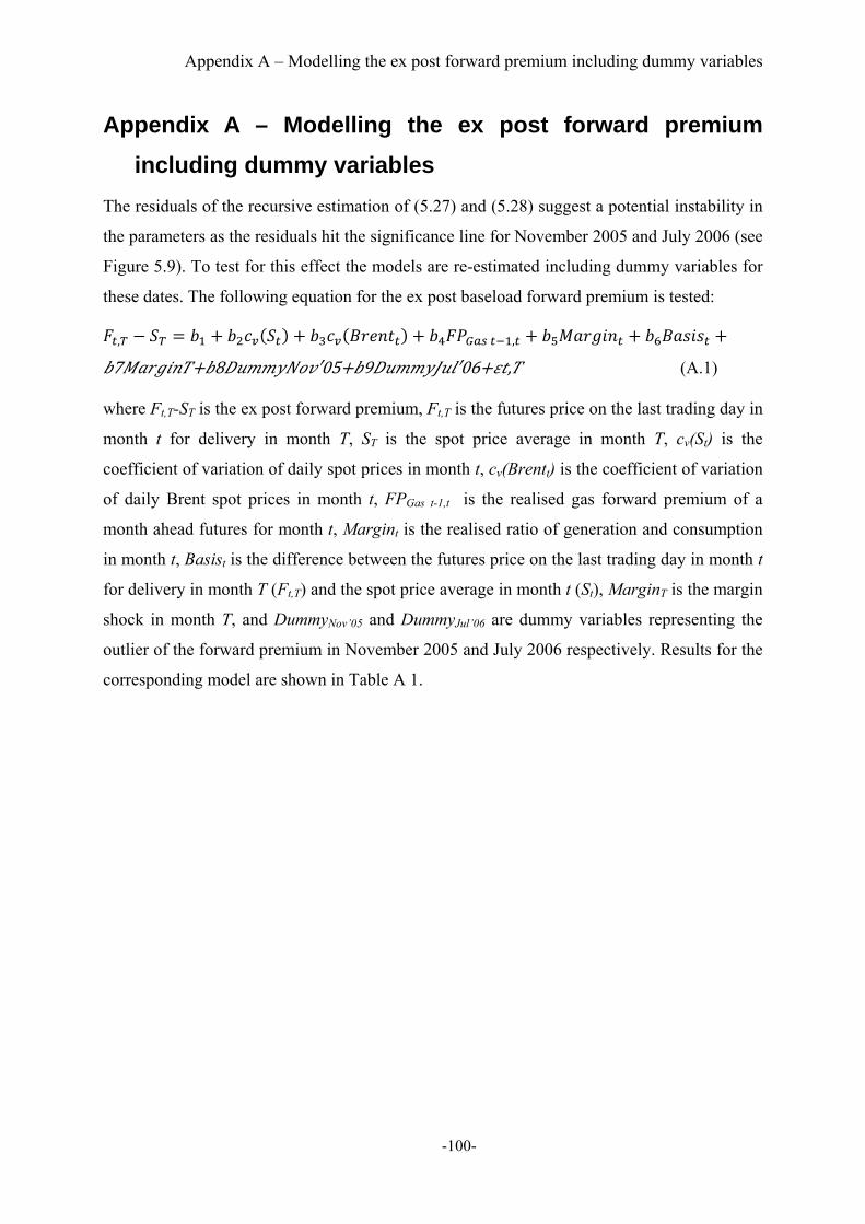
Appendix A – Modelling the ex post forward premium including dummy variables
-100-
Appendix A – Modelling the ex post forward premium
including dummy variables
The residuals of the recursive estimation of (5.27) and (5.28) suggest a potential instability in
the parameters as the residuals hit the significance line for November 2005 and July 2006 (see
Figure 5.9). To test for this effect the models are re-estimated including dummy variables for
these dates. The following equation for the ex post baseload forward premium is tested:
, ,
7 8 ′05 9 ′06 , (A.1)
where Ft,T-ST is the ex post forward premium, Ft,T is the futures price on the last trading day in
month t for delivery in month T, ST is the spot price average in month T, cv(St) is the
coefficient of variation of daily spot prices in month t, cv(Brentt) is the coefficient of variation
of daily Brent spot prices in month t, FPGas t-1,t is the realised gas forward premium of a
month ahead futures for month t, Margint is the realised ratio of generation and consumption
in month t, Basist is the difference between the futures price on the last trading day in month t
for delivery in month T (Ft,T) and the spot price average in month t (St), MarginT is the margin
shock in month T, and DummyNov’05 and DummyJul’06 are dummy variables representing the
outlier of the forward premium in November 2005 and July 2006 respectively. Results for the
corresponding model are shown in Table A 1.
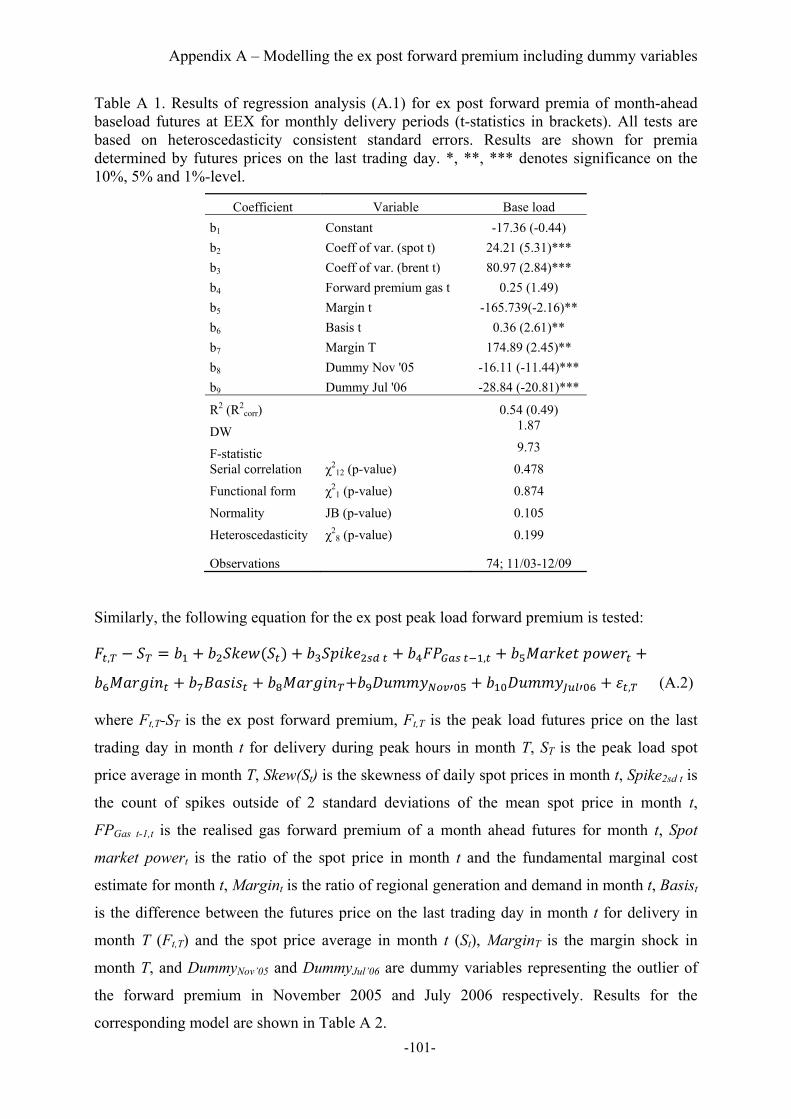
Appendix A – Modelling the ex post forward premium including dummy variables
-101-
Table A 1. Results of regression analysis (A.1) for ex post forward premia of month-ahead baseload futures at EEX for monthly delivery periods (t-statistics in brackets). All tests are based on heteroscedasticity consistent standard errors. Results are shown for premia determined by futures prices on the last trading day. *, **, *** denotes significance on the 10%, 5% and 1%-level.
Coefficient Variable Base load
b1 Constant -17.36 (-0.44)
b2 Coeff of var. (spot t) 24.21 (5.31)***
b3 Coeff of var. (brent t) 80.97 (2.84)***
b4 Forward premium gas t 0.25 (1.49)
b5 Margin t -165.739(-2.16)**
b6 Basis t 0.36 (2.61)**
b7 Margin T 174.89 (2.45)**
b8 Dummy Nov '05 -16.11 (-11.44)***
b9 Dummy Jul '06 -28.84 (-20.81)***
R2 (R2corr) 0.54 (0.49)
DW 1.87
F-statistic 9.73
Serial correlation χ212 (p-value) 0.478
Functional form χ21 (p-value) 0.874
Normality JB (p-value) 0.105
Heteroscedasticity χ28 (p-value) 0.199
Observations 74; 11/03-12/09
Similarly, the following equation for the ex post peak load forward premium is tested:
, ,
, (A.2)
where Ft,T-ST is the ex post forward premium, Ft,T is the peak load futures price on the last
trading day in month t for delivery during peak hours in month T, ST is the peak load spot
price average in month T, Skew(St) is the skewness of daily spot prices in month t, Spike2sd t is
the count of spikes outside of 2 standard deviations of the mean spot price in month t,
FPGas t-1,t is the realised gas forward premium of a month ahead futures for month t, Spot
market powert is the ratio of the spot price in month t and the fundamental marginal cost
estimate for month t, Margint is the ratio of regional generation and demand in month t, Basist
is the difference between the futures price on the last trading day in month t for delivery in
month T (Ft,T) and the spot price average in month t (St), MarginT is the margin shock in
month T, and DummyNov’05 and DummyJul’06 are dummy variables representing the outlier of
the forward premium in November 2005 and July 2006 respectively. Results for the
corresponding model are shown in Table A 2.
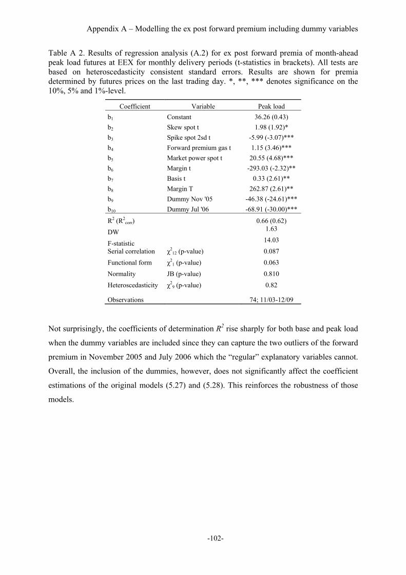
Appendix A – Modelling the ex post forward premium including dummy variables
-102-
Table A 2. Results of regression analysis (A.2) for ex post forward premia of month-ahead peak load futures at EEX for monthly delivery periods (t-statistics in brackets). All tests are based on heteroscedasticity consistent standard errors. Results are shown for premia determined by futures prices on the last trading day. *, **, *** denotes significance on the 10%, 5% and 1%-level.
Coefficient Variable Peak load
b1 Constant 36.26 (0.43)
b2 Skew spot t 1.98 (1.92)*
b3 Spike spot 2sd t -5.99 (-3.07)***
b4 Forward premium gas t 1.15 (3.46)***
b5 Market power spot t 20.55 (4.68)***
b6 Margin t -293.03 (-2.32)**
b7 Basis t 0.33 (2.61)**
b8 Margin T 262.87 (2.61)**
b9 Dummy Nov '05 -46.38 (-24.61)***
b10 Dummy Jul '06 -68.91 (-30.00)***
R2 (R2corr) 0.66 (0.62)
DW 1.63
F-statistic 14.03
Serial correlation χ212 (p-value) 0.087
Functional form χ21 (p-value) 0.063
Normality JB (p-value) 0.810
Heteroscedasticity χ29 (p-value) 0.82
Observations 74; 11/03-12/09
Not surprisingly, the coefficients of determination R2 rise sharply for both base and peak load
when the dummy variables are included since they can capture the two outliers of the forward
premium in November 2005 and July 2006 which the “regular” explanatory variables cannot.
Overall, the inclusion of the dummies, however, does not significantly affect the coefficient
estimations of the original models (5.27) and (5.28). This reinforces the robustness of those
models.
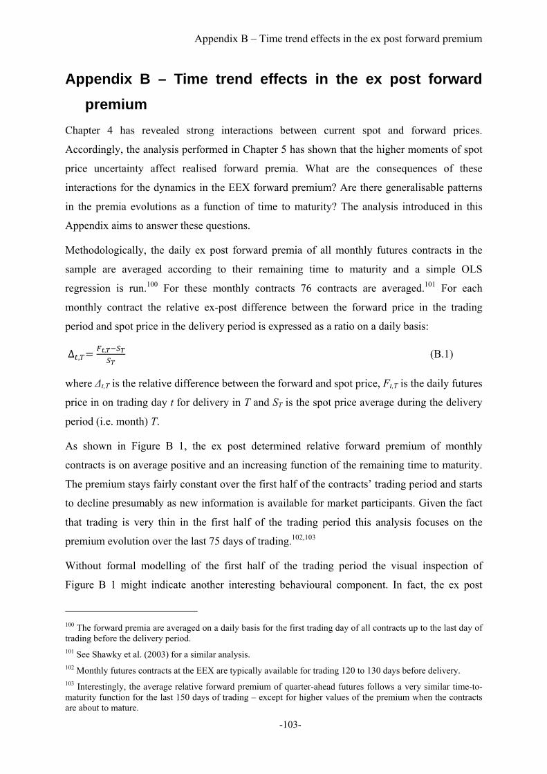
Appendix B – Time trend effects in the ex post forward premium
-103-
Appendix B – Time trend effects in the ex post forward
premium
Chapter 4 has revealed strong interactions between current spot and forward prices.
Accordingly, the analysis performed in Chapter 5 has shown that the higher moments of spot
price uncertainty affect realised forward premia. What are the consequences of these
interactions for the dynamics in the EEX forward premium? Are there generalisable patterns
in the premia evolutions as a function of time to maturity? The analysis introduced in this
Appendix aims to answer these questions.
Methodologically, the daily ex post forward premia of all monthly futures contracts in the
sample are averaged according to their remaining time to maturity and a simple OLS
regression is run.100 For these monthly contracts 76 contracts are averaged.101 For each
monthly contract the relative ex-post difference between the forward price in the trading
period and spot price in the delivery period is expressed as a ratio on a daily basis:
∆ ,, (B.1)
where Δt,T is the relative difference between the forward and spot price, Ft,T is the daily futures
price in on trading day t for delivery in T and ST is the spot price average during the delivery
period (i.e. month) T.
As shown in Figure B 1, the ex post determined relative forward premium of monthly
contracts is on average positive and an increasing function of the remaining time to maturity.
The premium stays fairly constant over the first half of the contracts’ trading period and starts
to decline presumably as new information is available for market participants. Given the fact
that trading is very thin in the first half of the trading period this analysis focuses on the
premium evolution over the last 75 days of trading.102,103
Without formal modelling of the first half of the trading period the visual inspection of
Figure B 1 might indicate another interesting behavioural component. In fact, the ex post
100 The forward premia are averaged on a daily basis for the first trading day of all contracts up to the last day of trading before the delivery period. 101 See Shawky et al. (2003) for a similar analysis. 102 Monthly futures contracts at the EEX are typically available for trading 120 to 130 days before delivery. 103 Interestingly, the average relative forward premium of quarter-ahead futures follows a very similar time-to-maturity function for the last 150 days of trading – except for higher values of the premium when the contracts are about to mature.
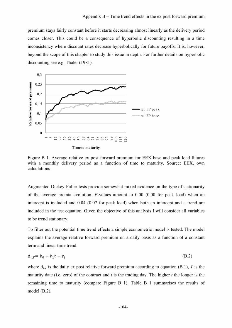
Appendix B – Time trend effects in the ex post forward premium
-104-
premium stays fairly constant before it starts decreasing almost linearly as the delivery period
comes closer. This could be a consequence of hyperbolic discounting resulting in a time
inconsistency where discount rates decrease hyperbolically for future payoffs. It is, however,
beyond the scope of this chapter to study this issue in depth. For further details on hyperbolic
discounting see e.g. Thaler (1981).
Figure B 1. Average relative ex post forward premium for EEX base and peak load futures with a monthly delivery period as a function of time to maturity. Source: EEX, own calculations
Augmented Dickey-Fuller tests provide somewhat mixed evidence on the type of stationarity
of the average premia evolution. P-values amount to 0.00 (0.00 for peak load) when an
intercept is included and 0.04 (0.07 for peak load) when both an intercept and a trend are
included in the test equation. Given the objective of this analysis I will consider all variables
to be trend stationary.
To filter out the potential time trend effects a simple econometric model is tested. The model
explains the average relative forward premium on a daily basis as a function of a constant
term and linear time trend:
∆ , (B.2)
where Δt,T is the daily ex post relative forward premium according to equation (B.1), T is the
maturity date (i.e. zero) of the contract and t is the trading day. The higher t the longer is the
remaining time to maturity (compare Figure B 1). Table B 1 summarises the results of
model (B.2).
0
0,05
0,1
0,15
0,2
0,25
0,3
1 8 15 22 29 36 43 50 57 64 71 78 85 92 9910
611
312
0
Rel
ativ
e fo
rwar
d pr
emiu
m
Time to maturity
rel. FP peak
rel. FP base
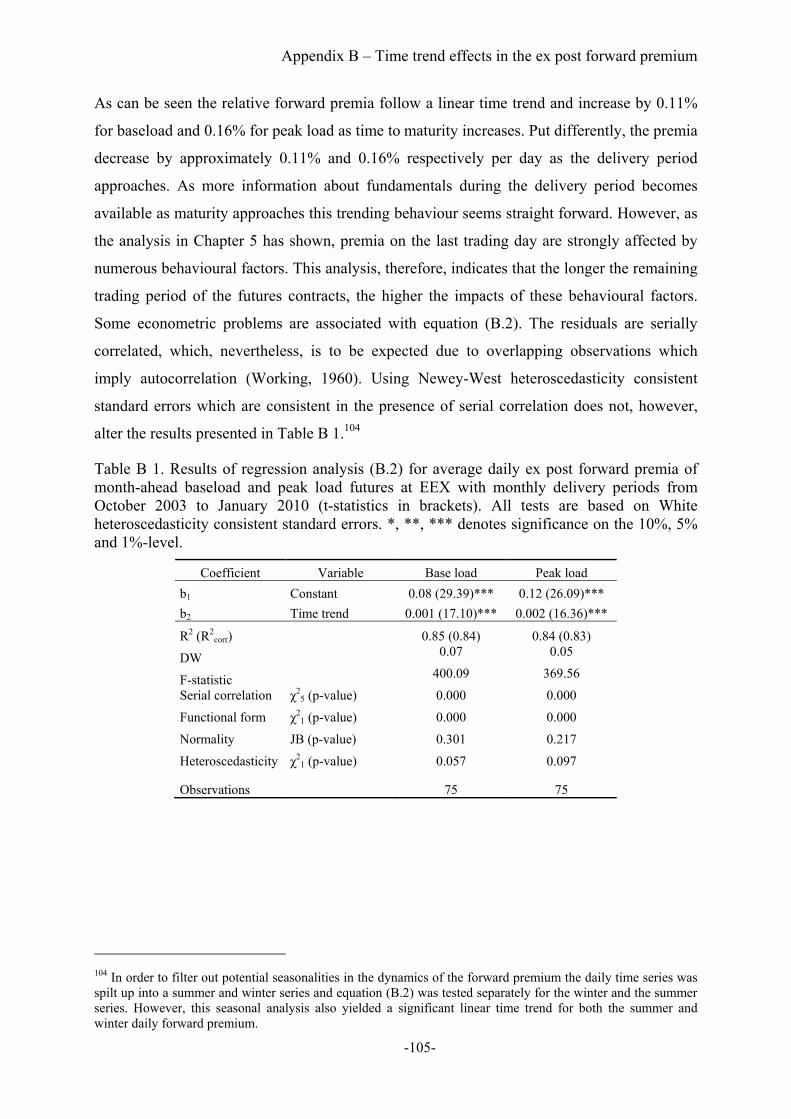
Appendix B – Time trend effects in the ex post forward premium
-105-
As can be seen the relative forward premia follow a linear time trend and increase by 0.11%
for baseload and 0.16% for peak load as time to maturity increases. Put differently, the premia
decrease by approximately 0.11% and 0.16% respectively per day as the delivery period
approaches. As more information about fundamentals during the delivery period becomes
available as maturity approaches this trending behaviour seems straight forward. However, as
the analysis in Chapter 5 has shown, premia on the last trading day are strongly affected by
numerous behavioural factors. This analysis, therefore, indicates that the longer the remaining
trading period of the futures contracts, the higher the impacts of these behavioural factors.
Some econometric problems are associated with equation (B.2). The residuals are serially
correlated, which, nevertheless, is to be expected due to overlapping observations which
imply autocorrelation (Working, 1960). Using Newey-West heteroscedasticity consistent
standard errors which are consistent in the presence of serial correlation does not, however,
alter the results presented in Table B 1.104
Table B 1. Results of regression analysis (B.2) for average daily ex post forward premia of month-ahead baseload and peak load futures at EEX with monthly delivery periods from October 2003 to January 2010 (t-statistics in brackets). All tests are based on White heteroscedasticity consistent standard errors. *, **, *** denotes significance on the 10%, 5% and 1%-level.
Coefficient Variable Base load Peak load
b1 Constant 0.08 (29.39)*** 0.12 (26.09)***
b2 Time trend 0.001 (17.10)*** 0.002 (16.36)***
R2 (R2corr) 0.85 (0.84) 0.84 (0.83)
DW 0.07 0.05
F-statistic 400.09 369.56
Serial correlation χ25 (p-value) 0.000 0.000
Functional form χ21 (p-value) 0.000 0.000
Normality JB (p-value) 0.301 0.217
Heteroscedasticity χ21 (p-value) 0.057 0.097
Observations 75 75
104 In order to filter out potential seasonalities in the dynamics of the forward premium the daily time series was spilt up into a summer and winter series and equation (B.2) was tested separately for the winter and the summer series. However, this seasonal analysis also yielded a significant linear time trend for both the summer and winter daily forward premium.

Appendix C – Derivation of the forward market equilibrium
-106-
Appendix C – Derivation of the forward market equilibrium
This Appendix derives the forward market equilibrium of section 2.3.2. The mean variance
utility function can be expanded to:
, , , , , , (C.1)
Using (2.5) the ex-post profit of producer i expands to:
(C.2)
Now the components of (C.1) can be calculated:
(C.3)
2 2 2
(C.4)
2 2 2 (C.5)
(C.4) and (C.5) yield
, (C.6)
Hence,
, (C.7)
which is text equation (2.8). The first order conditions give the profit maximising quantity
sold (or bought) in the forward market:
0 , (C.8)
, (C.9)
which is text equation (2.10).
Speculator j maximises the following profit equation:
(C.10)
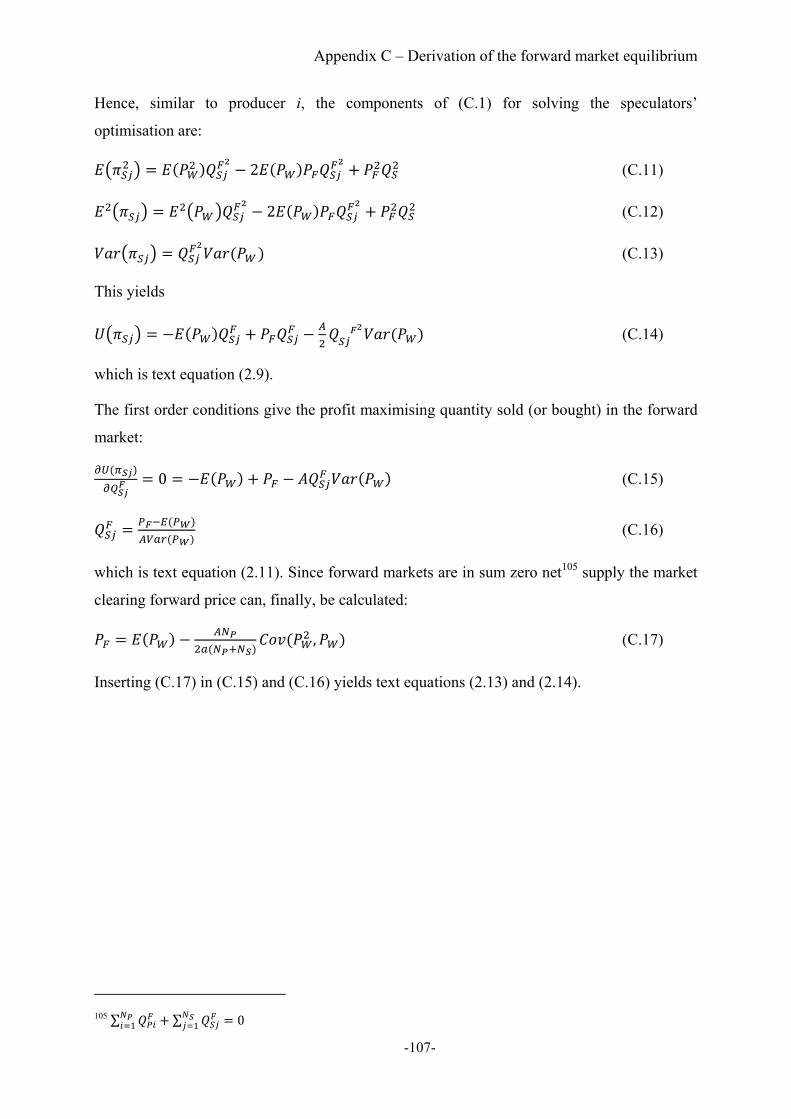
Appendix C – Derivation of the forward market equilibrium
-107-
Hence, similar to producer i, the components of (C.1) for solving the speculators’
optimisation are:
2 (C.11)
2 (C.12)
(C.13)
This yields
(C.14)
which is text equation (2.9).
The first order conditions give the profit maximising quantity sold (or bought) in the forward
market:
0 (C.15)
(C.16)
which is text equation (2.11). Since forward markets are in sum zero net105 supply the market
clearing forward price can, finally, be calculated:
, (C.17)
Inserting (C.17) in (C.15) and (C.16) yields text equations (2.13) and (2.14).
105 ∑ ∑ 0

Appendix D – Cournot duopoly equilibrium
-108-
Appendix D – Cournot duopoly equilibrium
This Appendix summarises the derivation of the standard Cournot duopoly solution referred
to in section 5.2.1.1. For further details see e.g. Henderson and Quandt (1980). For the case of
a single spot market the profit of the first duopolist equals
, , (D.1)
where PW is the wholesale price, QP1 denotes the quantity sold by producer 1 and TC1 are the
total cost associated with production of producer 1. Total costs are assumed to be linear,
, so is the inverse demand function . Given these
relations the reaction function of the Cournot producers can be derived:
,0 2 (D.2)
(D.3)
(D.4)
Solving for the spot market equilibrium by inserting (D.4) in (D.3) yields the well-known
Cournot duopoly solution:
(D.5)
(D.6)
which are text equations (5.11) and (5.12).

List of Tables
-109-
List of Tables
Table 3.1. Correlation coefficients between monthly averages of EEX and Nord Pool year-
ahead base load prices and explanatory variables from December 2004 to December 2009. . 23
Table 3.2. Results of regression analysis (3.2) for Δ Ln Year-ahead base load futures traded
during February 2005 to December 2009 at the EEX and Nord Pool exchanges (t-statistics in
brackets). All tests are based on heteroscedasticity consistent standard errors. *, **, ***
denotes significance on the 10%, 5% and 1%-level. ................................................................ 25
Table 3.3. Results of regression analysis (3.3) and (3.4) for Δ Ln Year-ahead base load futures
traded during December 2004 to December 2009 at the EEX and Nord Pool exchanges (t-
statistics in brackets). All tests are based on heteroscedasticity consistent standard errors. *,
**, *** denotes significance on the 10%, 5% and 1%-level. ................................................... 31
Table 4.1. Correlation coefficients between daily EEX spot, month-ahead, quarter-ahead and
year-ahead base load prices noted on working days (top panel) from September 2003 to
December 2009 and summary statistics (bottom panel). ......................................................... 37
Table 4.2. Correlation coefficients between daily EEX spot and futures returns (top panel)
from September 2003 to December 2009 and summary statistics (bottom panel). ................. 38
Table 4.3. Results of the unrestricted VAR model (4.2) for daily spot and forward prices of
EEX from September 2003 to December 2009 (t-statistics in brackets). *, **, *** denotes
significance on the 10%, 5% and 1%-level. ............................................................................. 39
Table 4.4. Results of Granger non-causality tests for daily spot and forward returns of EEX
from September 2003 to December 2009. ............................................................................... 40
Table 4.5 Results of the unrestricted VAR model (4.3) for daily electricity spot and forward
price returns at the EEX from July 2007 to December 2009 (t-statistics in brackets). *, **, ***
denotes significance on the 10%, 5% and 1%-level. ................................................................ 42
Table 5.1. Summary statistics of the relative differences of monthly averages and prices on
the last trading day of EEX month-ahead futures (with delivery from October 2003 to January
2010) and average spot prices in the respective delivery period. ............................................. 61
Table 5.2. Results of regression analysis (5.26) for ex post forward premia of month-ahead
baseload and peak load futures at EEX and Nord Pool with monthly delivery periods from
November 2003 to January 2010 (t-statistics in brackets). All tests are based on
List of Tables
-110-
heteroscedasticity consistent standard errors. Results are shown for premia determined by
futures prices on the last trading day. ....................................................................................... 64
Table 5.3. Summary of forward premia determinants. * denotes that the respective variables
are observable for market participants on the forward trading day. ......................................... 71
Table 5.4. Results of regression analysis (5.27) for ex post forward premia of month-ahead
baseload futures at EEX for monthly delivery periods (t-statistics in brackets). All tests are
based on heteroscedasticity consistent standard errors. Results are shown for premia
determined by futures prices on the last trading day. *, **, *** denotes significance on the
10%, 5% and 1%-level. ............................................................................................................ 73
Table 5.5. Results of regression analysis (5.28) for ex post forward premia of month-ahead
peak load futures at EEX for monthly delivery periods (t-statistics in brackets). All tests are
based on heteroscedasticity consistent standard errors. Results are shown for premia
determined by futures prices on the last trading day. *, **, *** denotes significance on the
10%, 5% and 1%-level. ............................................................................................................ 75
Table 5.6. Effect of temperature surprises on the realised ex post forward premium for winter
and summer months. ................................................................................................................ 82
Table 5.7. Results of regression analysis (5.29) for ex post forward premia of month-ahead
baseload futures at EEX for monthly delivery periods (t-statistics in brackets). All tests are
based on heteroscedasticity consistent standard errors. Results are shown for premia
determined by futures prices on the last trading day. *, **, *** denotes significance on the
10%, 5% and 1%-level ............................................................................................................. 84
Table 5.8. Results of regression analysis (5.30) for ex post forward premia of month-ahead
peak load futures at EEX for monthly delivery periods (t-statistics in brackets). All tests are
based on heteroscedasticity consistent standard errors. Results are shown for premia
determined by futures prices on the last trading day. *, **, *** denotes significance on the
10%, 5% and 1%-level ............................................................................................................. 86

List of Figures
-111-
List of Figures
Figure 2.1. Price formation in a competitive electricity market. For the low and high demand
case the wholesale prices, Plow and Phigh respectively, equals system marginal costs. That is,
the short run generation costs of the most expensive plant needed to meet demand. ................ 8
Figure 2.2. Equilibrium of forward and expected spot prices. Source: Borenstein et al. (2008) 9
Figure 2.3. Probability density function of expected profits of producer i when relying solely
on the spot market (left) and when hedging profits by contracting on the forward market as
well (right). ............................................................................................................................... 16
Figure 2.4. Relative forward premium as a function of relative demand standard deviation. . 17
Figure 3.1. European electricity markets, corresponding wholesale price averages in 2009 and
bottlenecks in the cross-border transmission grids. Source: Various power exchanges .......... 19
Figure 3.2. Average yearly wholesale prices in the Western European Power market. Source:
Various power exchanges ......................................................................................................... 19
Figure 3.3. Evolution of monthly averages of spot and forward prices for base load electricity
at EEX and Nord Pool. Source: EEX, Nord Pool .................................................................... 20
Figure 3.4. Monthly averages of year-ahead coal, gas and CO2 emission allowance prices vs.
EEX and Nord Pool year-ahead base load futures. Source: EEX, Nord Pool .......................... 22
Figure 3.5. CUSUM and CUSUM of squares test for regression model (3.2) for EEX (left)
and Nord Pool (right). .............................................................................................................. 26
Figure 3.6. Recursive estimates of the coefficients of model (3.2) for EEX ........................... 28
Figure 3.7. Recursive estimates of the coefficients of model (3.2) for Nord Pool .................. 29
Figure 4.1. Comparison of daily spot prices (grey line) and daily forward settlement prices for
the next month, quarter and year (coloured lines). Note that the y-axis is restricted to values
ranging from 20 to 120 €/MWh. Source: EEX ........................................................................ 35
Figure 4.2. Daily spot price and forward price (month, quarter and year-ahead) returns.
Source: EEX, own calculations ................................................................................................ 37
Figure 4.3. Pair wise Granger causality for daily electricity spot and futures price returns at
the EEX. ................................................................................................................................... 40
List of Figures
-112-
Figure 5.1. Effects of introducing a forward market in a Cournot type market. Left: Market
without contracts. Right: Market where QF was sold beforehand on the forward market.
Source: Based on Willems (2004) ............................................................................................ 52
Figure 5.2. Evolution of monthly averages of peak load spot prices (black) and peak load
month-ahead futures prices on the last trading day (grey) at the EEX from October 2003 to
January 2010. Source: EEX ..................................................................................................... 58
Figure 5.3 Descriptive statistics and histogram of daily base (top) and peak load spot prices
(bottom) at the EEX from October 2003 to January 2010. Daily baseload prices are the
averages of all 24 hourly prices each day. Daily peak load prices are calculated Monday’s to
Friday’s as the average of the hourly prices from 8:00am to 8:00pm. ..................................... 59
Figure 5.4. Relative differences of month-ahead peak load futures prices (noted on the last
trading day) with respect to the actual spot price during the delivery period at the EEX from
October 2003 to January 2010. Source: EEX, own calculations ............................................. 60
Figure 5.5. Effects of the convexity of the supply curve on price changes due to similar
deviations of the supply and demand curves in base load (off-peak) versus peak load. .......... 61
Figure 5.6. Seasonal graph of realised monthly percentage peak load forward premia at the
EEX. ......................................................................................................................................... 62
Figure 5.7. Evolution of electricity prices (average baseload price at the EEX) and system
marginal costs in the regional EU-4-market from October 2003 to December 2009. Source:
EEX, BAFA, UCTE, own calculations .................................................................................... 69
Figure 5.8. CUSUM and CUSUM of squares test for regression models (5.27) (baseload
model, left) and (5.28) (peak load model, right) applied to EEX month-ahead forward premia
.................................................................................................................................................. 77
Figure 5.9. Recursive residuals for regression models (6.26 – baseload model, left) and (6.27
– peak load model, right) applied to EEX month-ahead forward premia ................................ 78
Figure 5.10. Recursive estimates of the coefficients of model (5.27) for baseload forward
premia at the EEX .................................................................................................................... 79
Figure 5.11. Recursive estimates of the coefficients of model (5.28) for peak load forward
premia at the EEX .................................................................................................................... 80
Figure 5.12. Temperature surprises (absolute values: black line and left scale; relative values:
grey line and right scale) in the delivery months of the forward contracts computed as

List of Figures
-113-
differences to the historic long term values. Source: http://www.engr.udayton.edu/weather/,
own calculations ....................................................................................................................... 81
Figure 5.13. Inframarginal generation surprises (absolute values: black line and left scale;
relative values: grey line and right scale) in the delivery months of the forward contracts
computed as differences to the historic long term values. Source: ENTSOE, own calculations
.................................................................................................................................................. 83


