econstor www.econstor.eu
Der Open-Access-Publikationsserver der ZBW – Leibniz-Informationszentrum WirtschaftThe Open Access Publication Server of the ZBW – Leibniz Information Centre for Economics
Standard-Nutzungsbedingungen:
Die Dokumente auf EconStor dürfen zu eigenen wissenschaftlichenZwecken und zum Privatgebrauch gespeichert und kopiert werden.
Sie dürfen die Dokumente nicht für öffentliche oder kommerzielleZwecke vervielfältigen, öffentlich ausstellen, öffentlich zugänglichmachen, vertreiben oder anderweitig nutzen.
Sofern die Verfasser die Dokumente unter Open-Content-Lizenzen(insbesondere CC-Lizenzen) zur Verfügung gestellt haben sollten,gelten abweichend von diesen Nutzungsbedingungen die in der dortgenannten Lizenz gewährten Nutzungsrechte.
Terms of use:
Documents in EconStor may be saved and copied for yourpersonal and scholarly purposes.
You are not to copy documents for public or commercialpurposes, to exhibit the documents publicly, to make thempublicly available on the internet, or to distribute or otherwiseuse the documents in public.
If the documents have been made available under an OpenContent Licence (especially Creative Commons Licences), youmay exercise further usage rights as specified in the indicatedlicence.
zbw Leibniz-Informationszentrum WirtschaftLeibniz Information Centre for Economics
Angelov, Nikolay; Johansson, Per; Lindahl, Erica
Working Paper
Gender differences in sickness absence and thegender division of family responsibilities
Working Paper, IFAU - Institute for Evaluation of Labour Market and Education Policy, No.2013:9
Provided in Cooperation with:IFAU - Institute for Evaluation of Labour Market and Education Policy,Uppsala
Suggested Citation: Angelov, Nikolay; Johansson, Per; Lindahl, Erica (2013) : Genderdifferences in sickness absence and the gender division of family responsibilities, WorkingPaper, IFAU - Institute for Evaluation of Labour Market and Education Policy, No. 2013:9
This Version is available at:http://hdl.handle.net/10419/82270
Gender differences in sickness absence and the gender division
of family responsibilities
Nikolay Angelov Per Johansson
Erica Lindahl
WORKING PAPER 2013:9
The Institute for Evaluation of Labour Market and Education Policy (IFAU) is a research institute under the Swedish Ministry of Employment, situated in Uppsala. IFAU’s objective is to promote, support and carry out scientific evaluations. The assignment includes: the effects of labour market and educational policies, studies of the functioning of the labour market and the labour market effects of social insurance policies. IFAU shall also disseminate its results so that they become accessible to different interested parties in Sweden and abroad. IFAU also provides funding for research projects within its areas of interest. The deadline for applications is October 1 each year. Since the researchers at IFAU are mainly economists, researchers from other disciplines are encouraged to apply for funding. IFAU is run by a Director-General. The institute has a scientific council, consisting of a chairman, the Director-General and five other members. Among other things, the scientific council proposes a decision for the allocation of research grants. A reference group including representatives for employer organizations and trade unions, as well as the ministries and authorities concerned is also connected to the institute. Postal address: P.O. Box 513, 751 20 Uppsala Visiting address: Kyrkogårdsgatan 6, Uppsala Phone: +46 18 471 70 70 Fax: +46 18 471 70 71 [email protected] www.ifau.se Papers published in the Working Paper Series should, according to the IFAU policy, have been discussed at seminars held at IFAU and at least one other academic forum, and have been read by one external and one internal referee. They need not, however, have undergone the standard scrutiny for publication in a scientific journal. The purpose of the Working Paper Series is to provide a factual basis for public policy and the public policy discussion. ISSN 1651-1166
Gender differences in sickness absence and thegender division of family responsibilities a
by
Nikolay Angelovb, Per Johanssonc and Erica Lindahld
17th April, 2013
AbstractThis study investigates possible reasons for the gender difference in sickness absence.We estimate both short- and long-term effects of parenthood in a within-couple analy-sis based on the timing of parenthood. We find that after entering parenthood, womenincrease their sickness absence by between 0.5 days per month (during the child’s thirdyear) and 0.85 days per month (during year 17) more than their spouse. By investigatingpossible explanations for the observed effect, we conclude that the effect mainly stemsfrom higher home commitment, which reduces women’s labour market attachment and,in turn, increases female sickness absence.
Keywords: Double burden, Health investment, Household work, Labour market work,Moral hazard, Parenthood, Sickness insurance, Work absenceJEL-codes: C23; D13; I19; J22
aWe are grateful for comments during seminars at IFAU, UCLS, and the Ministry of Social Affairs, aswell as from participants at the Workshop on absenteeism and social insurance (Utrecht, September 2011).Financial support from the Swedish Council for Working Life and Social Research (DNR 2004-2005) isgratefully acknowledged.
bThe Institute for Labour Market and Education Policy Evaluation (IFAU) and Uppsala Center for LabourStudies (UCLS); [email protected]
cThe Institute for Labour Market and Education Policy Evaluation (IFAU), the Department of Economics,Uppsala University and IZA; [email protected]
dThe Institute for Labour Market and Education Policy Evaluation (IFAU); [email protected].
IFAU – Gender differences in sickness absence and the gender division of family responsibilities 1
Table of contens
1 Introduction . . . . . . . . . . . . . . . . . . . . . . . . . . . . . . . . . . . . . . . . . . . . . . . . . . . . . . . . . . . . . . . . . . . . . . . . . . 3
2 The gender gap in sickness absence and labour supply . . . . . . . . . . . . . . . . . . . . . . . . . . . . 6
3 The Swedish social insurance . . . . . . . . . . . . . . . . . . . . . . . . . . . . . . . . . . . . . . . . . . . . . . . . . . . . . . . 103.1 General principles. . . . . . . . . . . . . . . . . . . . . . . . . . . . . . . . . . . . . . . . . . . . . . . . . . . . . . . . . . . . . . . . . . . . 103.2 Sickness benefits . . . . . . . . . . . . . . . . . . . . . . . . . . . . . . . . . . . . . . . . . . . . . . . . . . . . . . . . . . . . . . . . . . . . . 113.3 Parental benefit and temporary parental benefits . . . . . . . . . . . . . . . . . . . . . . . . . . . . . . . . . . . 11
4 Empirical strategy, data, descriptive statistics, and graphical evidence . . . . . . . . . . . 124.1 The empirical strategy . . . . . . . . . . . . . . . . . . . . . . . . . . . . . . . . . . . . . . . . . . . . . . . . . . . . . . . . . . . . . . . 124.2 Data . . . . . . . . . . . . . . . . . . . . . . . . . . . . . . . . . . . . . . . . . . . . . . . . . . . . . . . . . . . . . . . . . . . . . . . . . . . . . . . . . . . 154.3 Descriptive statistics . . . . . . . . . . . . . . . . . . . . . . . . . . . . . . . . . . . . . . . . . . . . . . . . . . . . . . . . . . . . . . . . . 174.4 Graphical evidence. . . . . . . . . . . . . . . . . . . . . . . . . . . . . . . . . . . . . . . . . . . . . . . . . . . . . . . . . . . . . . . . . . . 17
5 Results . . . . . . . . . . . . . . . . . . . . . . . . . . . . . . . . . . . . . . . . . . . . . . . . . . . . . . . . . . . . . . . . . . . . . . . . . . . . . . . . 195.1 Main results . . . . . . . . . . . . . . . . . . . . . . . . . . . . . . . . . . . . . . . . . . . . . . . . . . . . . . . . . . . . . . . . . . . . . . . . . . 195.2 Sensitivity analysis. . . . . . . . . . . . . . . . . . . . . . . . . . . . . . . . . . . . . . . . . . . . . . . . . . . . . . . . . . . . . . . . . . . 235.2.1 Subsequent births . . . . . . . . . . . . . . . . . . . . . . . . . . . . . . . . . . . . . . . . . . . . . . . . . . . . . . . . . . . . . . . . . . . . 235.2.2 Composition of sickness benefit eligible individuals. . . . . . . . . . . . . . . . . . . . . . . . . . . . . . . 26
6 Family responsibilities and sickness absence. . . . . . . . . . . . . . . . . . . . . . . . . . . . . . . . . . . . . . . 266.1 A gender differential change in health . . . . . . . . . . . . . . . . . . . . . . . . . . . . . . . . . . . . . . . . . . . . . . 276.2 Economic incentives . . . . . . . . . . . . . . . . . . . . . . . . . . . . . . . . . . . . . . . . . . . . . . . . . . . . . . . . . . . . . . . . . 286.3 Empirical results . . . . . . . . . . . . . . . . . . . . . . . . . . . . . . . . . . . . . . . . . . . . . . . . . . . . . . . . . . . . . . . . . . . . . 296.3.1 Health. . . . . . . . . . . . . . . . . . . . . . . . . . . . . . . . . . . . . . . . . . . . . . . . . . . . . . . . . . . . . . . . . . . . . . . . . . . . . . . . . 296.3.2 Economic incentives . . . . . . . . . . . . . . . . . . . . . . . . . . . . . . . . . . . . . . . . . . . . . . . . . . . . . . . . . . . . . . . . . 30
7 Conclusion . . . . . . . . . . . . . . . . . . . . . . . . . . . . . . . . . . . . . . . . . . . . . . . . . . . . . . . . . . . . . . . . . . . . . . . . . . . 33
2 IFAU – Gender differences in sickness absence and the gender division of family responsibilities
1 IntroductionWomen are more absent from work for health reasons than men (see e.g., Paringer, 1983;
Brostrom et al., 2004; Mastekaasa and Olsen, 1998, and Bratberg et al., 2002). This ob-
servation is in line with other observed gender differences on morbidity measures such
as health care utilization and self reported health (see e.g., Sindelar, 1982). One interest-
ing aspect of the gender difference in work absence for health reasons, denoted sickness
absence in the following, is its strong correlation over time with the gender difference in
labor supply (see Figures 3 and 4 in section 2). This provides suggestive evidence that
the gender difference is not primarily driven by health differences, but rather connected
to the increased female labor supply over the last 40 years.1
Today, the dual earner family is the most common family form in the OECD coun-
tries.2 Family responsibilities are, however, not equally shared; instead, women tend to
perform dual tasks (see e.g. Boye, 2008; Booth and Ours, 2005; Evertsson and Nermo,
2007; Tichenor, 1999). Women are active on the labour market and they perform the ma-
jority of the household production, while men predominantly specialize in market work.
More effort at home would in general mean less time and effort for labour market work.
This is also what we observe. Time use studies in Sweden have consistently shown that
labour market work is higher for men but that total time worked (household and labour
market) of men and women are approximately the same (SCB, 2009). This result corre-
sponds well with time-use studies in USA, Germany and the Netherlands (Burda et al.,
2008).
It is also empirically established that the unequal gender division of household and
market work emerges when couples get their first child (Van der Lippe and Siegers, 1994;
Sanchez and Thomson 1997, Gauthier and Furstenberg, 2002; Gjerdingen and Center
2005; Baxter et al. 2008) and that women decrease their labor supply after childbirth
1The global average gender gap in life expectancy is four years (cf. Lee, 2010) and in Sweden the gap is al-most 5 years (The World Factbook, 2012). This observed morbidity-mortality paradox (see also Nathanson,1975 and Verbrugge, 1982) is also in line with the idea that the gender gap in sickness absence is not pri-marily driven by gender health differences.
2The median employment rate for partnered mothers in the OECD countries was 66.5 percent in 2007 (OECD2010) and according to U.S. Bureau of Labor Statistics (2011), the U.S. labor force participation rate ofmothers with children under 18 years of age was 71.3 percent in March 2010.
IFAU – Gender differences in sickness absence and the gender division of family responsibilities 3
(e.g., Angrist and Evans, 1998 and Jacobsen, Wishart, and Rosenbloom, 1999) while
fathers, if anything, even do the opposite (Kennerberg, 2007).
From this perspective it is of interest to study the effects of the unequal sharing of the
new commitment at home after becoming parents, or in other words, to study the effects
of women’s dual role on different outcomes. This paper studies whether there is a gender
difference in the effect of parenthood on sickness absence behaviour. To this end, we
compare the evolution of the within-couple gender gap in sickness absence before and
after the arrival of the first child. The empirical analysis is based on detailed universal
Swedish administrative registers. These data allow us to track parents’ sickness absence3
over a significant part of their labour market career, starting a few years before parenthood
up to 18 years after the arrival of the first child.
To our knowledge, this is the first study of the effect of parenthood on sickness ab-
sence. A related study is Akerlind et al. (1996), who estimate gender differences in
sickness absence at different ages separately for individuals with and without children.
More closely related are two studies that focus on the effect of household responsibility
on sickness absence. Bratberg et al. (2002) suggest that the gender gap in sickness ab-
sence stems from the psychological pressure of the dual role, or in other words, what they
denote a double burden among women. In their empirical analysis, Bratberg et al. (2002)
use the number of children as a proxy for family responsibilities. Paringer (1983), on the
other hand, argues that women’s dual role as both producers on the labour market and
at home (in contrast to the more labour market specialized man) implies that women’s
health is more important for the household than men’s, since a household would suffer
more than just forgone earnings if the female is ill. In the empirical analysis, Paringer uses
marital status as a proxy for household responsibilities and finds that, married women are
less absent from work for health reasons than unmarried women, contrary to what theory
predicts.
Estimating a causal effect of family responsibilities on sickness absence by using mar-
3Sickness absence is defined as days with sickness benefits paid by the Swedish Social Insurance Agency.The first two weeks are paid for by the employer if the insured individual is employed. The length of theemployer-payment period has varied over time from 2 to 3 weeks. In all estimations we control for thisvariation over time with year dummies.
4 IFAU – Gender differences in sickness absence and the gender division of family responsibilities
ital status or number of children as proxy variables is associated with methodological chal-
lenges. The basic problem is to separate the effects of marital status or number of children
from potentially correlated factors that also might affect sickness absence. Marital status
and the number of children are both positively correlated with household responsibilities,
but they are probably also correlated with health; women who are married or have (many)
children at a given age probably have better health and might thereby be less absent due
to sickness than non-married women or women without (or with few) children.
In this study, we take advantage of detailed register data, which allow us to use the
timing of parenthood in the identification of both short- and long-term effects of parent-
hood on sickness absence. By focusing on the within-couple difference over time, we
do not have to rely on cross-sectional comparisons and we control for both observed and
unobserved factors correlated with parenthood and sickness absence.
Our main finding is that entering parenthood on average increases mothers’ sickness
absence in comparison with fathers’. Before the arrival of the first child, there is no
significant difference between the genders. During the child’s third year, when most of
the mothers are back at work, women are about 0.5 days per month more absent due to
own sickness than men. This gender gap persists and gradually increases as long as data
allow us to follow the parents, i.e., 17 years after the first born child’s birth the gender gap
is about 0.85 days per month. This result holds for several sensitivity analyses, including
different model specifications, controlling for subsequent births and restricting the sample
in various ways with respect to the maximum number of children and the income level
of the parents. A graphical analysis suggests that the effect stems from an increase in
sickness absence among women and no corresponding increase among men.
We discuss two possible explanations for the observed gender differences in sickness
absence after parenthood. The first explanation focuses on gender differences in health.
On the one hand, physiological pressure among women due to their dual responsibility
(cf. Bratberg et al., 2002) may cause health deterioration. On the other hand, this dual
responsibility may lead to an increased investment in health, as suggested by Paringer
(1983), thereby causing a relative improvement in female health. The second explanation
concerns changes in economic incentives for labour market work after entering parent-
IFAU – Gender differences in sickness absence and the gender division of family responsibilities 5
hood. The conclusion from an analysis of this explanation is that reduced labour market
attachment among women after entering parenthood is an important explanatory factor
for the gender gap in sickness absence.
This paper is organized as follows. Section 2 provides some background informa-
tion about the development on the Swedish labour market during the latest decades with
respect to sickness absence and labour market participation. Section 3 describes the
Swedish social insurance system. Section 4 formalizes the empirical framework and
gives some basic descriptive statistics and some first-glance graphical evidence. Section 5
presents the main results and in section 6, we discuss and present empirical evidence for
possible explanations for the observed gender differences. Finally, section 7 concludes
the paper.
2 The gender gap in sickness absence and laboursupply
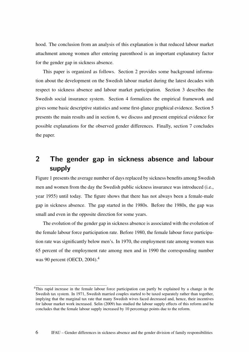
Figure 1 presents the average number of days replaced by sickness benefits among Swedish
men and women from the day the Swedish public sickness insurance was introduced (i.e.,
year 1955) until today. The figure shows that there has not always been a female-male
gap in sickness absence. The gap started in the 1980s. Before the 1980s, the gap was
small and even in the opposite direction for some years.
The evolution of the gender gap in sickness absence is associated with the evolution of
the female labour force participation rate. Before 1980, the female labour force participa-
tion rate was significantly below men’s. In 1970, the employment rate among women was
65 percent of the employment rate among men and in 1990 the corresponding number
was 90 percent (OECD, 2004).4
4This rapid increase in the female labour force participation can partly be explained by a change in theSwedish tax system. In 1971, Swedish married couples started to be taxed separately rather than together,implying that the marginal tax rate that many Swedish wives faced decreased and, hence, their incentivesfor labour market work increased. Selin (2009) has studied the labour supply effects of this reform and heconcludes that the female labour supply increased by 10 percentage points due to the reform.
6 IFAU – Gender differences in sickness absence and the gender division of family responsibilities
1015
2025
Year
Day
s on
sic
k le
ave
per
pers
on a
nd y
ear
1955 1963 1971 1979 1987 1995 2003
WomenMen
Figure 1: The average number of sick-leave days with sickness benefits per person (ages 16–65) andyear in Sweden, divided upon men and women.Source: Statistics Sweden.
Although we lack exact information on which group of women that entered the labour
market in the 1960s and in the 1970s, several facts suggest that it was, at least partly,
driven by mothers with young children. During the 1970s and 1980s, the Swedish parental
leave system became more generous and the public provided child-care expanded rapidly.
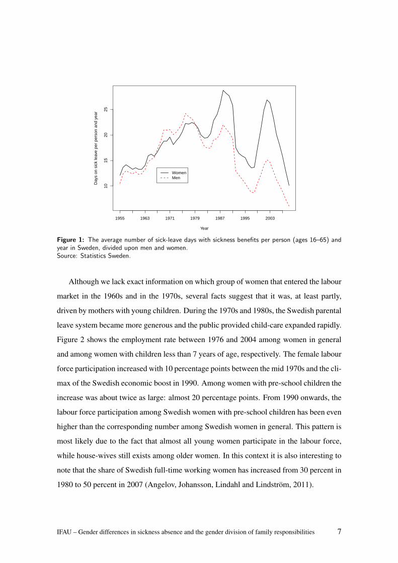
Figure 2 shows the employment rate between 1976 and 2004 among women in general
and among women with children less than 7 years of age, respectively. The female labour
force participation increased with 10 percentage points between the mid 1970s and the cli-
max of the Swedish economic boost in 1990. Among women with pre-school children the
increase was about twice as large: almost 20 percentage points. From 1990 onwards, the
labour force participation among Swedish women with pre-school children has been even
higher than the corresponding number among Swedish women in general. This pattern is
most likely due to the fact that almost all young women participate in the labour force,
while house-wives still exists among older women. In this context it is also interesting to
note that the share of Swedish full-time working women has increased from 30 percent in
1980 to 50 percent in 2007 (Angelov, Johansson, Lindahl and Lindstrom, 2011).
IFAU – Gender differences in sickness absence and the gender division of family responsibilities 7
0.65
0.70
0.75
0.80
0.85
Year
Sha
re e
mpl
oyed
am
ong
wom
en
1976 1980 1984 1988 1992 1996 2000 2004
WomenWomen with children < 7 years
Figure 2: Labor force participation among all Swedish women and among women with children under7 years between 1976 and 2004. Source: Statistics Sweden.Source: Statistics Sweden.
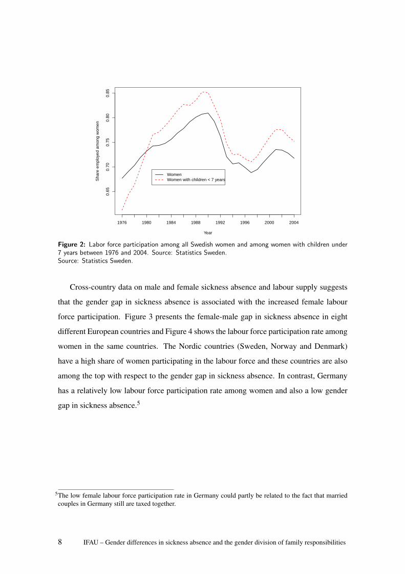
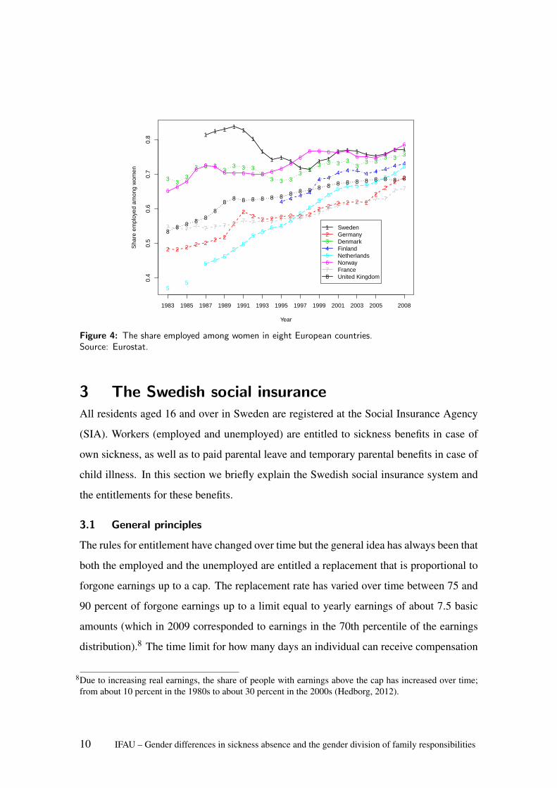
Cross-country data on male and female sickness absence and labour supply suggests
that the gender gap in sickness absence is associated with the increased female labour
force participation. Figure 3 presents the female-male gap in sickness absence in eight
different European countries and Figure 4 shows the labour force participation rate among
women in the same countries. The Nordic countries (Sweden, Norway and Denmark)
have a high share of women participating in the labour force and these countries are also
among the top with respect to the gender gap in sickness absence. In contrast, Germany
has a relatively low labour force participation rate among women and also a low gender
gap in sickness absence.5
5The low female labour force participation rate in Germany could partly be related to the fact that marriedcouples in Germany still are taxed together.
8 IFAU – Gender differences in sickness absence and the gender division of family responsibilities
−0.
20.
00.
20.
40.
60.
81.
0
Year
Gen
der
gap
in s
hare
abs
ent
1983 1985 1987 1989 1991 1993 1995 1997 1999 2001 2003 2005 2008
1 11
11
11 1 1
1
1
1
1 1
11
11
11
1 1
2
2
22
22
22 2 2 2 2
2
2
2
22
2 22
2 22 2 2
3
3
33
3
33 3
33 3
3
3
3
3
3 3 3
3
3
3
3
3
33
3
4
4
4
4
4 44
4
4
4
4
4
4
45
5
5
5
5
5
55
5
5
55 5
55
5 55
55 5 5 5
5
6
6
6
6 6
6
6
6 66 6
6 6
6
6
6
66 6
6 6
6
6 66
6
7 77
77
7
7
7
7
7
7
77
7
7
7 7 7 77
7 77
7
77
88 8
8
88
88
8
8
88
88
8 8
8
8 8
8
8
8 88
88
12345678
SwedenGermanyDenmarkFinlandNetherlandsNorwayFranceUnited Kingdom
Figure 3: i) The percentage female-male gap in sickness absence during a study-period of one weekamong employed workers in eight European countries.Source: Eurostat.
Swedish women do not leave the labour market when they enter parenthood. However,
they do take the large majority of the parental leave and they utilize the generous Swedish
parental leave system and work part-time while having small children. In Sweden, 80
percent of the paid parental leave is taken by women (Forsakringskassan, 2011)6 and
44 percent of all women in the ages 25-54 work part-time (¡35 hours per week).7 The
corresponding share of men who work part-time is 10 percent.
6During the first 18 months with a baby both parents can stay at home on a full-time basis with job-protection.Thereafter, parents are allowed to reduce their working hours up to 25 percent until the child turns 8 yearsold (SFS 1995:584).
7Public statistics from Statistics Sweden, published on the web: http://www.scb.se/Pages/Article____332715.aspx
IFAU – Gender differences in sickness absence and the gender division of family responsibilities 9
0.4
0.5
0.6
0.7
0.8
Year
Sha
re e
mpl
oyed
am
ong
wom
en
1983 1985 1987 1989 1991 1993 1995 1997 1999 2001 2003 2005 2008
11 1 1
1
1
11 1
11 1
1 11 1 1 1 1 1
1 1
2 2 2 2 2 2 2
2
22 2 2 2 2 2 2
2 2 2 2 2 22
22
23 33
3 3 33
3 3 33
3 3 33
33 3 3 3
33 3
3 3 3
4 4 4 4
4 44 4 4 4 4 4
4 4
55
55
55
55
55 5
55
55
55 5 5 5 5
55
5
66
6
66 6
6 6 6 6 6 6 66
66 6 6 6 6
6 6 66
66
7 7 77 7 7 7 7 7 7 7 7 7 7 7 7 7
7 7 7 7 7 7 77 7
88 8 8 8
8
88 8 8 8 8 8 8 8 8 8 8 8 8 8 8 8 8 8 8
12345678
SwedenGermanyDenmarkFinlandNetherlandsNorwayFranceUnited Kingdom
Figure 4: The share employed among women in eight European countries.Source: Eurostat.
3 The Swedish social insuranceAll residents aged 16 and over in Sweden are registered at the Social Insurance Agency
(SIA). Workers (employed and unemployed) are entitled to sickness benefits in case of
own sickness, as well as to paid parental leave and temporary parental benefits in case of
child illness. In this section we briefly explain the Swedish social insurance system and
the entitlements for these benefits.
3.1 General principles
The rules for entitlement have changed over time but the general idea has always been that
both the employed and the unemployed are entitled a replacement that is proportional to
forgone earnings up to a cap. The replacement rate has varied over time between 75 and
90 percent of forgone earnings up to a limit equal to yearly earnings of about 7.5 basic
amounts (which in 2009 corresponded to earnings in the 70th percentile of the earnings
distribution).8 The time limit for how many days an individual can receive compensation
8Due to increasing real earnings, the share of people with earnings above the cap has increased over time;from about 10 percent in the 1980s to about 30 percent in the 2000s (Hedborg, 2012).
10 IFAU – Gender differences in sickness absence and the gender division of family responsibilities
from the SIA depends on the reason for the absence.
3.2 Sickness benefits
In case of illness, the first day is not replaced. Thereafter the employer pays sick-pay for
the 14 following days. After 14 days the SIA disburses sickness benefits. For unemployed
persons the SIA starts disbursing sickness benefits from the second day onwards. In this
study, we focus on sickness absence with sickness benefit. That means that for employees,
we start counting the number of days absent from the first day in the third week within a
given illness period. (For unemployed persons we start counting the second day in a sick-
spell, i.e., when the SIA enters.) Thus, the type of sickness absence we have in mind in
this study is not short-term sickness absence but a longer-lasting reduced working capacity
(usually longer than 14 days).9
Compensation for illness periods longer than 7 days requires a medical certificate
from a physician with information about the expected length of the sick leave. Based on
this certificate, the SIA formally decides whether an individual is entitled compensation
or not. When the entitled period has expired, a renewal certificate is required and the
process is repeated. A person can be on sickness benefit for at most 364 days during 15
months. If work capacity is still reduced after a year, a person can apply for extended
sickness benefit, which could, at the time, continue without time limit.10
Although the formal decision about sickness benefits is made by the SIA, the sickness
benefit claimant can influence the outcome. According to Arrelov et al. (2006), the
outcome is largely controlled by the insured’s motivation. Englund (2001) also finds
that doctors believe that they prescribe too long sickness-absence durations, that is, the
duration is not always motivated by medical consideration.
3.3 Parental benefit and temporary parental benefits
Parents receive parental benefits if they stay at home for child-care instead of working on
the labour market.11 Parental benefits are payable for 450 days for each child. One parent
9In the analysis we condition on some annual labour market income. Thus, persons who are full-time unem-ployed during a whole year are not included.
10In 2008 a time limit of one year for the use of sickness benefit was introduced.11This holds also for persons without earnings who receive a flat rate of 60 SEK (approx. 6 Euro) per day.
IFAU – Gender differences in sickness absence and the gender division of family responsibilities 11
may give up the right to parental benefit to the other parent, with the exception of 60 days.
Parents with children under 8 years old age are also entitled to unpaid job-protected leave
with a great portion of flexibility. During the child’s first 18 months both parents can stay
at home on a full-time basis with job-protection. Thereafter, parents are allowed to reduce
their working hours up to 25 percent until the child turns 8 years old (SFS 1995:584).
In addition to parental benefits, parents are entitled to temporary parental benefits if
they have to stay at home to care for an ill child under the age of 12.12 Parents are together
eligible for temporary parental benefits for 60 days per child and year. After these 60 days,
a further sixty days can be taken, if the need for these extra days has been approved by
the SIA.
Work absence due to child illness is financially more beneficial than work absence due
to own illness since it is compensated for the first day of work absence. Until recently,
there was no formal monitoring of absence due to child care. Engstrom et al. (2007) show
that this disharmony between the two insurances leads to a large excess use of temporary
benefits and Persson (2011) finds that this also leads to unintended flows from sickness
insurance benefits to temporary parental benefits.13 Thus, if anything, days on sickness
benefits are an underreported measure of work absence.14
4 Empirical strategy, data, descriptive statistics, andgraphical evidence
4.1 The empirical strategy
There are several challenges associated with estimating the effect of parenthood on work
absence due to own sickness. First, it is reasonable to believe that the likelihood of having
a child, as well as the timing of when a couple decides to have a child, is correlated with
health and labour market success. Second, the spouses probably affect each other. To this
12This also applies if the person who normally looks after the child falls ill.13The first report started a lively debate in Sweden about cheating parents, and on the 1st of July 2008 the
rules were changed. As a result, until recently, the day-care centre had to confirm – via a special certificate– that the child has been absent before the SIA pays out temporary parental benefit.
14This study focuses on sickness absence longer than 14 days. Thus, the extent of flows from sickness benefitsto the temporary parental benefits should be small.
12 IFAU – Gender differences in sickness absence and the gender division of family responsibilities
end, we restrict the analysis to the estimation of an effect of parenthood on the gender
difference in sickness absence for those becoming parents.
By asking how the within-couple gender gap changes when a couple enters parent-
hood, we control for a lot of unobserved individual characteristics that might be corre-
lated with parenthood. In order to be clear on the identification strategy, it is formalized
in Appendix A. The take-home message from Appendix A is that we are able to identify
the effect of parenthood on the gender gap in sickness absence under the assumption that
the expected potential gender gap in sickness absence in the absence of a child is constant
for our population.
The following discussion will hopefully make the identification assumption palatable.
Both groups (men and women) are affected by the intervention (entering parenthood),
but we allow the magnitude of the effect to differ between the genders. The identifying
assumption is the same as in a traditional difference-in-differences setting, i.e., the inter-
vention must be strictly exogenous. That is, the timing of when to have a child should not
be determined by expected shocks to the within-family gender difference in sickness ab-
sence the couple would have experienced in absence of entering parenthood. This means
that the timing of entering parenthood should not be influenced by, for us, unobservable
information about sickness absence changes of men in comparison to women or vice
versa.
Although we find no differences in sickness absence before entering parenthood, there
are several reasons to believe that also men and women without children would differ in
their sickness absence behaviour. Women have, for instance, lower average earnings.
Since there is a cap in the insurance this means that, on average, women face higher real
replacement rates than men. Another potential reason for different take up rates among
men and women can be the highly gender segregated Swedish labour market (see, e.g.,
SOU, 2004). However, in general, the work environment for the males is worse than the
work environment for the females (see e.g. Brostrom et al., 2004, Angelov et al., 2011
and Mastekaasa and Olsen, 2000), which suggests a gender gap in the opposite direction
than the one we observe in data. By using the pre-birth within-household differences we
control for potential differences due to a gender segregated labour market. Another caveat
IFAU – Gender differences in sickness absence and the gender division of family responsibilities 13
is that the gender segregated labour market might imply gender differential business cycle
effects, which are important to control for. That is why we estimate the effect by ordinary
least squares (OLS), which allows us to control for business cycle effects. We also control
for a restricted set of potential confounders that may affect the timing of parenthood and
difference in take up rates of sickness benefits. To this end, we control for differences in
education, income and age.
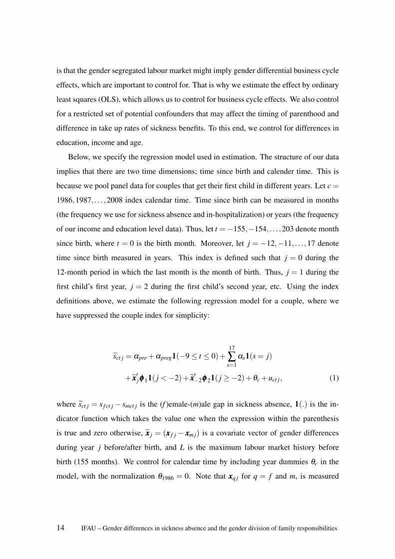
Below, we specify the regression model used in estimation. The structure of our data
implies that there are two time dimensions; time since birth and calender time. This is
because we pool panel data for couples that get their first child in different years. Let c =
1986,1987, . . . ,2008 index calendar time. Time since birth can be measured in months
(the frequency we use for sickness absence and in-hospitalization) or years (the frequency
of our income and education level data). Thus, let t =−155,−154, . . . ,203 denote month
since birth, where t = 0 is the birth month. Moreover, let j = −12,−11, . . . ,17 denote
time since birth measured in years. This index is defined such that j = 0 during the
12-month period in which the last month is the month of birth. Thus, j = 1 during the
first child’s first year, j = 2 during the first child’s second year, etc. Using the index
definitions above, we estimate the following regression model for a couple, where we
have suppressed the couple index for simplicity:
sct j = αpre +αpreg111(−9≤ t ≤ 0)+17
∑s=1
αs111(s = j)
+ xxx′jφφφ 1111( j <−2)+ xxx′−2φφφ 2111( j ≥−2)+θc +uct j, (1)
where sct j = s f ct j− smct j is the (f )emale-(m)ale gap in sickness absence, 111(.) is the in-
dicator function which takes the value one when the expression within the parenthesis
is true and zero otherwise, xxx j = (xxx f j− xxxm j) is a covariate vector of gender differences
during year j before/after birth, and L is the maximum labour market history before
birth (155 months). We control for calendar time by including year dummies θc in the
model, with the normalization θ1986 = 0. Note that xxxq j for q = f and m, is measured
14 IFAU – Gender differences in sickness absence and the gender division of family responsibilities
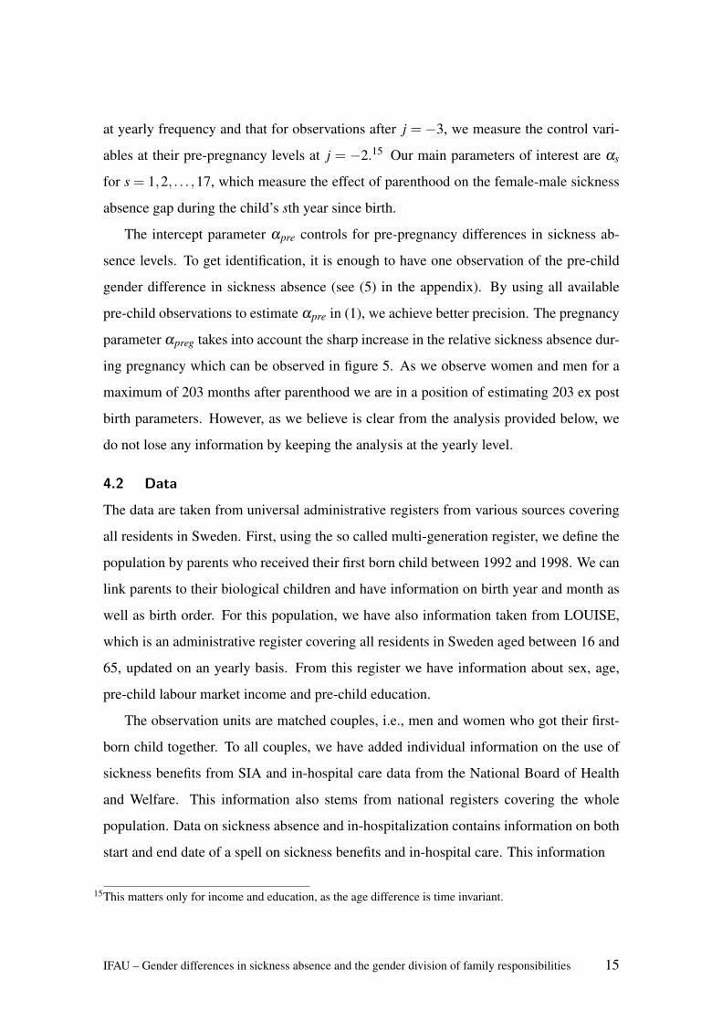
at yearly frequency and that for observations after j = −3, we measure the control vari-
ables at their pre-pregnancy levels at j = −2.15 Our main parameters of interest are αs
for s = 1,2, . . . ,17, which measure the effect of parenthood on the female-male sickness
absence gap during the child’s sth year since birth.
The intercept parameter αpre controls for pre-pregnancy differences in sickness ab-
sence levels. To get identification, it is enough to have one observation of the pre-child
gender difference in sickness absence (see (5) in the appendix). By using all available
pre-child observations to estimate αpre in (1), we achieve better precision. The pregnancy
parameter αpreg takes into account the sharp increase in the relative sickness absence dur-
ing pregnancy which can be observed in figure 5. As we observe women and men for a
maximum of 203 months after parenthood we are in a position of estimating 203 ex post
birth parameters. However, as we believe is clear from the analysis provided below, we
do not lose any information by keeping the analysis at the yearly level.
4.2 Data
The data are taken from universal administrative registers from various sources covering
all residents in Sweden. First, using the so called multi-generation register, we define the
population by parents who received their first born child between 1992 and 1998. We can
link parents to their biological children and have information on birth year and month as
well as birth order. For this population, we have also information taken from LOUISE,
which is an administrative register covering all residents in Sweden aged between 16 and
65, updated on an yearly basis. From this register we have information about sex, age,
pre-child labour market income and pre-child education.
The observation units are matched couples, i.e., men and women who got their first-
born child together. To all couples, we have added individual information on the use of
sickness benefits from SIA and in-hospital care data from the National Board of Health
and Welfare. This information also stems from national registers covering the whole
population. Data on sickness absence and in-hospitalization contains information on both
start and end date of a spell on sickness benefits and in-hospital care. This information
15This matters only for income and education, as the age difference is time invariant.
IFAU – Gender differences in sickness absence and the gender division of family responsibilities 15
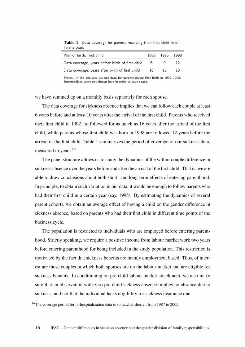
Table 1: Data coverage for parents receiving their first child in dif-ferent years
Year of birth, first child 1992 1995 1998
Data coverage, years before birth of first child 6 9 12
Data coverage, years after birth of first child 16 13 10
Notes: In the analysis, we use data for parents giving first birth in 1992–1998.Intermediate years not shown here in order to save space.
we have summed up on a monthly basis separately for each spouse.
The data coverage for sickness absence implies that we can follow each couple at least
6 years before and at least 10 years after the arrival of the first child. Parents who received
their first child in 1992 are followed for as much as 16 years after the arrival of the first
child, while parents whose first child was born in 1998 are followed 12 years before the
arrival of the first child. Table 1 summarizes the period of coverage of our sickness data,
measured in years.16
The panel structure allows us to study the dynamics of the within-couple difference in
sickness absence over the years before and after the arrival of the first child. That is, we are
able to draw conclusions about both short- and long-term effects of entering parenthood.
In principle, to obtain such variation in our data, it would be enough to follow parents who
had their first child in a certain year (say, 1995). By estimating the dynamics of several
parent cohorts, we obtain an average effect of having a child on the gender difference in
sickness absence, based on parents who had their first child in different time points of the
business cycle.
The population is restricted to individuals who are employed before entering parent-
hood. Strictly speaking, we require a positive income from labour market work two years
before entering parenthood for being included in the study population. This restriction is
motivated by the fact that sickness benefits are mainly employment based. Thus, of inter-
est are those couples in which both spouses are on the labour market and are eligible for
sickness benefits. In conditioning on pre-child labour market attachment, we also make
sure that an observation with zero pre-child sickness absence implies no absence due to
sickness, and not that the individual lacks eligibility for sickness insurance due
16The coverage period for in-hospitalization data is somewhat shorter, from 1987 to 2005.
16 IFAU – Gender differences in sickness absence and the gender division of family responsibilities
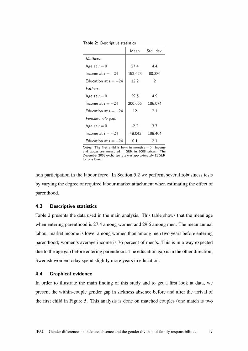
Table 2: Descriptive statistics
Mean Std. dev.
Mothers:
Age at t = 0 27.4 4.4
Income at t =−24 152,023 80,386
Education at t =−24 12.2 2
Fathers:
Age at t = 0 29.6 4.9
Income at t =−24 200,066 106,074
Education at t =−24 12 2.1
Female-male gap:
Age at t = 0 -2.2 3.7
Income at t =−24 -48,043 108,404
Education at t =−24 0.1 2.1
Notes: The first child is born in month t = 0. Incomeand wages are measured in SEK in 2008 prices. TheDecember 2008 exchange rate was approximately 11 SEKfor one Euro.
non participation in the labour force. In Section 5.2 we perform several robustness tests
by varying the degree of required labour market attachment when estimating the effect of
parenthood.
4.3 Descriptive statistics
Table 2 presents the data used in the main analysis. This table shows that the mean age
when entering parenthood is 27.4 among women and 29.6 among men. The mean annual
labour market income is lower among women than among men two years before entering
parenthood; women’s average income is 76 percent of men’s. This is in a way expected
due to the age gap before entering parenthood. The education gap is in the other direction;
Swedish women today spend slightly more years in education.
4.4 Graphical evidence
In order to illustrate the main finding of this study and to get a first look at data, we
present the within-couple gender gap in sickness absence before and after the arrival of
the first child in Figure 5. This analysis is done on matched couples (one match is two
IFAU – Gender differences in sickness absence and the gender division of family responsibilities 17
parents who got their first child together). Using monthly sickness-absence data, we can
follow some parents for as long as 155 months before their first child is born (January
1986 to December 1998 for children born in December 1998) and another fraction for
203 months after (January 1992 to December 2008 for children born in January, 1992).
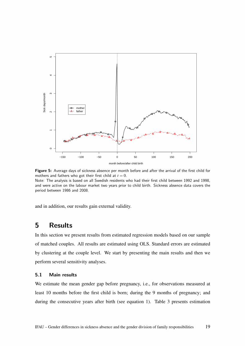
The data plotted in Figure 5 represent raw monthly average sickness absence for matched
couples who received their first child during the period 1992 to 1998. The spike in female
sickness absence occurs before the birth of the first child. This increase in absence is due
to problems during pregnancy. During the period directly after child birth, we observe a
dramatic decrease in sickness absence for women and during this period mothers are even
less absent than fathers. This is most likely because most mothers take use of the paid
maternity leave during the child’s first year. The main message of this study is however
summarized by the difference in evolution of sickness absence occurring two years after
the birth of the first child. The gender gap in sickness absence is large and persistent for
as long as we can follow the couples.
It should be noted that besides the visible variation of the gender gap in sickness ab-
sence over time since birth (on the x-axis), Figure 5 also contains some variation over
calendar time (cf. Figure 1). In the empirical analysis that follows, we are able to control
for this calendar-year variation, since we use parents who received their first child in var-
ious years. This is an important aspect of our data, which allows us to identify the effect
of parenthood on the gender gap in sickness absence separately from calendar-year vari-
ation. For instance, using data for couples who received their first child in one particular
year, the effect could be confounded with different labour market shocks or diseases that
affect women and men differently. Although if it is very unlikely that the confounders are
perfectly correlated with the short-run dynamics of the effect of parenthood (i.e., the pre-
birth spike and the decrease during the first year Figure 5), the long-term effect estimates
might be contaminated by calendar time shocks, if we only use couples who received their
first child during a specific year. Another possible drawback of using parents from one
particular year would be the external validity of our results. Thus, by using parents who
received their first child in different years, we are able to control for potential confounders,
18 IFAU – Gender differences in sickness absence and the gender division of family responsibilities
−150 −100 −50 0 50 100 150 200
01
23
45
month before/after child birth
Sic
k da
ys/m
onth
motherfather
Figure 5: Average days of sickness absence per month before and after the arrival of the first child formothers and fathers who got their first child at t = 0.Note: The analysis is based on all Swedish residents who had their first child between 1992 and 1998,and were active on the labour market two years prior to child birth. Sickness absence data covers theperiod between 1986 and 2008.
and in addition, our results gain external validity.
5 ResultsIn this section we present results from estimated regression models based on our sample
of matched couples. All results are estimated using OLS. Standard errors are estimated
by clustering at the couple level. We start by presenting the main results and then we
perform several sensitivity analyses.
5.1 Main results
We estimate the mean gender gap before pregnancy, i.e., for observations measured at
least 10 months before the first child is born; during the 9 months of pregnancy; and
during the consecutive years after birth (see equation 1). Table 3 presents estimation
IFAU – Gender differences in sickness absence and the gender division of family responsibilities 19
results from three different specifications. The first column presents estimates without
any controls. In the second column, we add controls for calendar years, and in the third
column, we also include controls for the age difference within each couple as well as
pre-child differences in income and years of education. All controls are measured at the
latest two years before the birth of the first child. All three specifications in Table 3 tell
the same story and all estimates are significant at the one percent level; in the long run,
the female-male gender gap in sickness absence increased due to parenthood. Before
explaining the interpretation of each regression coefficient, we discuss how the different
model specifications affect the long-term estimate of the gender gap in sickness absence.
As already noted, there has been a substantial variation in the overall gender gap in
sickness absence during our study period (see Figure 1). Including calendar year controls
reduces the magnitude of the estimated effects for years 3 through 13 since the birth of the
first child and leaves the rest of the estimates virtually unchanged. Adding age and pre-
child controls does not change the results, except for the intercept term which captures
the mean difference before pregnancy. In the model with calendar year controls only, the
intercept is negative and not statistically significant. In the third column when control
variables are added, the intercept is marginally positive (0.04 days more per month) and
statistically significant at the 5 percent level. All in all, we believe this provides some
evidence of similar trends in sickness absence before entering parenthood, once we have
controlled for calendar year effects.
In the following we discuss the estimates in the third column (qualitatively we have
the same results in the second column however). The results confirm what was already
seen from the graphical analysis displayed in Figure 5. Pregnancy increases the gender
gap in sickness absence drastically: the effect is 1.7 days per month during this period.
This increase is arguably due to mothers’ pregnancy-related illnesses. During the first
year after birth, the difference is instead negative, i.e., fathers are on average more absent
due to sickness than mothers: -0.16 days per month. This is most likely because most
mothers are on paid maternity leave during the child’s first year. During this period of
maternity leave there is in general no need to take use of the sickness insurance in order
20 IFAU – Gender differences in sickness absence and the gender division of family responsibilities
to be absent from work for health reasons.17
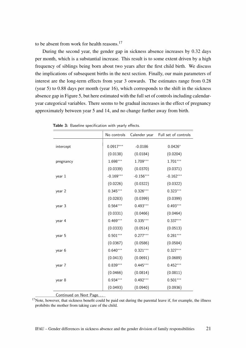
During the second year, the gender gap in sickness absence increases by 0.32 daysper month, which is a substantial increase. This result is to some extent driven by a highfrequency of siblings being born about two years after the first child birth. We discussthe implications of subsequent births in the next section. Finally, our main parameters ofinterest are the long-term effects from year 3 onwards. The estimates range from 0.28(year 5) to 0.88 days per month (year 16), which corresponds to the shift in the sicknessabsence gap in Figure 5, but here estimated with the full set of controls including calendar-year categorical variables. There seems to be gradual increases in the effect of pregnancyapproximately between year 5 and 14, and no change further away from birth.
Table 3: Baseline specification with yearly effects.
No controls Calender year Full set of controls
intercept 0.0917∗∗∗ -0.0186 0.0426∗
(0.0138) (0.0184) (0.0204)
pregnancy 1.698∗∗∗ 1.709∗∗∗ 1.701∗∗∗
(0.0339) (0.0370) (0.0371)
year 1 -0.169∗∗∗ -0.156∗∗∗ -0.162∗∗∗
(0.0226) (0.0322) (0.0322)
year 2 0.345∗∗∗ 0.326∗∗∗ 0.323∗∗∗
(0.0283) (0.0399) (0.0399)
year 3 0.564∗∗∗ 0.493∗∗∗ 0.493∗∗∗
(0.0331) (0.0466) (0.0464)
year 4 0.469∗∗∗ 0.335∗∗∗ 0.337∗∗∗
(0.0333) (0.0514) (0.0513)
year 5 0.501∗∗∗ 0.277∗∗∗ 0.281∗∗∗
(0.0367) (0.0586) (0.0584)
year 6 0.640∗∗∗ 0.321∗∗∗ 0.327∗∗∗
(0.0413) (0.0691) (0.0689)
year 7 0.839∗∗∗ 0.445∗∗∗ 0.452∗∗∗
(0.0466) (0.0814) (0.0811)
year 8 0.934∗∗∗ 0.492∗∗∗ 0.501∗∗∗
(0.0493) (0.0940) (0.0936)
Continued on Next Page. . .17Note, however, that sickness benefit could be paid out during the parental leave if, for example, the illness
prohibits the mother from taking care of the child.
IFAU – Gender differences in sickness absence and the gender division of family responsibilities 21
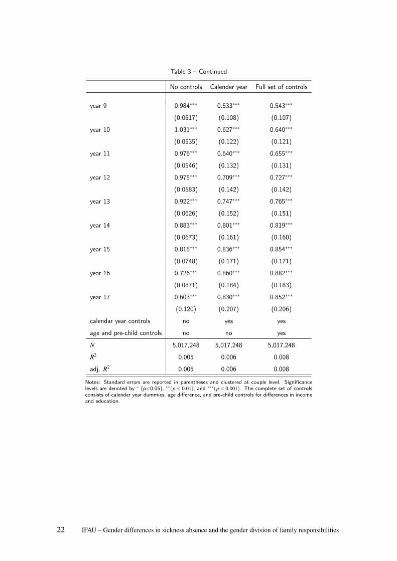
Table 3 – Continued
No controls Calender year Full set of controls
year 9 0.984∗∗∗ 0.533∗∗∗ 0.543∗∗∗
(0.0517) (0.108) (0.107)
year 10 1.031∗∗∗ 0.627∗∗∗ 0.640∗∗∗
(0.0535) (0.122) (0.121)
year 11 0.976∗∗∗ 0.640∗∗∗ 0.655∗∗∗
(0.0546) (0.132) (0.131)
year 12 0.975∗∗∗ 0.709∗∗∗ 0.727∗∗∗
(0.0583) (0.142) (0.142)
year 13 0.922∗∗∗ 0.747∗∗∗ 0.765∗∗∗
(0.0626) (0.152) (0.151)
year 14 0.883∗∗∗ 0.801∗∗∗ 0.819∗∗∗
(0.0673) (0.161) (0.160)
year 15 0.815∗∗∗ 0.836∗∗∗ 0.854∗∗∗
(0.0748) (0.171) (0.171)
year 16 0.726∗∗∗ 0.860∗∗∗ 0.882∗∗∗
(0.0871) (0.184) (0.183)
year 17 0.603∗∗∗ 0.830∗∗∗ 0.852∗∗∗
(0.120) (0.207) (0.206)
calendar year controls no yes yes
age and pre-child controls no no yes
N 5,017,248 5,017,248 5,017,248
R2 0.005 0.006 0.008
adj. R2 0.005 0.006 0.008
Notes: Standard errors are reported in parentheses and clustered at couple level. Significancelevels are denoted by ∗ (p<0.05), ∗∗(p < 0.01), and ∗∗∗(p < 0.001). The complete set of controlsconsists of calender year dummies, age difference, and pre-child controls for differences in incomeand education.
22 IFAU – Gender differences in sickness absence and the gender division of family responsibilities
5.2 Sensitivity analysis
In this section we address two concerns: subsequent births and the composition of indi-
viduals eligible for sickness benefit. The pregnancy itself and the days around the birth
are associated with a sharp increase in the sickness absence gap. Thus, the shift in the
sickness absence after the birth of the first child could potentially be explained by subse-
quent births and short-term pregnancy-related illnesses. On the other hand, the estimated
effect during year 1 is negative, suggesting a short-term negative effect of giving birth.
Moreover, although we condition on being eligible for sickness benefit before entering
parenthood, parenthood could cause women to leave the labour force. If anything, this
would attenuate the estimated effect toward zero. To investigate these issues, we present
several sensitivity analyses below.
5.2.1 Subsequent births
We start by investigating how a second child affects the gender gap in sickness absence.
In this analysis, the first-child dummy captures sickness absence differences only as long
as the mother is not pregnant with her second child. As soon as the second pregnancy
begins (i.e., 9 months before the birth of the second child), the second-child pregnancy
dummy captures the sickness absence difference. The first column in Table 4 presents
the results from this analysis. The first-child estimates now capture the dynamics of the
gender gap in sickness absence for a) the minority of couples that only get one child
during the period, and b) the period after the birth of the first child and before the birth of
the second child among the majority of couples who get a second child. In contrast, the
variation used to estimate the second-child parameter stems solely from couples that get
a second child.
The long-term effects (for year 3 since the birth of the first child and thereafter) are
estimated using a dummy variable that has the value one if a) more than two years have
passed since the birth of the first child, and b) for couples that get a second child, either
more than two years have passed since the second birth, or the mother is not yet pregnant
IFAU – Gender differences in sickness absence and the gender division of family responsibilities 23
with the second child.18
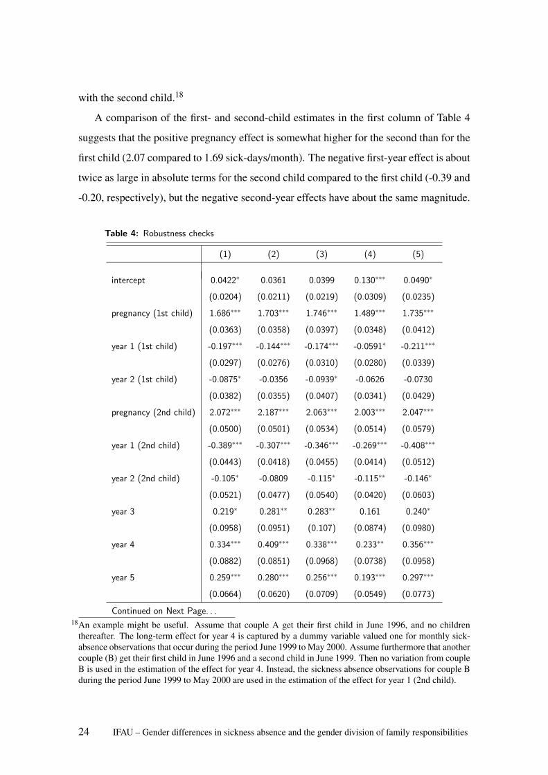
A comparison of the first- and second-child estimates in the first column of Table 4
suggests that the positive pregnancy effect is somewhat higher for the second than for the
first child (2.07 compared to 1.69 sick-days/month). The negative first-year effect is about
twice as large in absolute terms for the second child compared to the first child (-0.39 and
-0.20, respectively), but the negative second-year effects have about the same magnitude.
Table 4: Robustness checks
(1) (2) (3) (4) (5)
intercept 0.0422∗ 0.0361 0.0399 0.130∗∗∗ 0.0490∗
(0.0204) (0.0211) (0.0219) (0.0309) (0.0235)
pregnancy (1st child) 1.686∗∗∗ 1.703∗∗∗ 1.746∗∗∗ 1.489∗∗∗ 1.735∗∗∗
(0.0363) (0.0358) (0.0397) (0.0348) (0.0412)
year 1 (1st child) -0.197∗∗∗ -0.144∗∗∗ -0.174∗∗∗ -0.0591∗ -0.211∗∗∗
(0.0297) (0.0276) (0.0310) (0.0280) (0.0339)
year 2 (1st child) -0.0875∗ -0.0356 -0.0939∗ -0.0626 -0.0730
(0.0382) (0.0355) (0.0407) (0.0341) (0.0429)
pregnancy (2nd child) 2.072∗∗∗ 2.187∗∗∗ 2.063∗∗∗ 2.003∗∗∗ 2.047∗∗∗
(0.0500) (0.0501) (0.0534) (0.0514) (0.0579)
year 1 (2nd child) -0.389∗∗∗ -0.307∗∗∗ -0.346∗∗∗ -0.269∗∗∗ -0.408∗∗∗
(0.0443) (0.0418) (0.0455) (0.0414) (0.0512)
year 2 (2nd child) -0.105∗ -0.0809 -0.115∗ -0.115∗∗ -0.146∗
(0.0521) (0.0477) (0.0540) (0.0420) (0.0603)
year 3 0.219∗ 0.281∗∗ 0.283∗∗ 0.161 0.240∗
(0.0958) (0.0951) (0.107) (0.0874) (0.0980)
year 4 0.334∗∗∗ 0.409∗∗∗ 0.338∗∗∗ 0.233∗∗ 0.356∗∗∗
(0.0882) (0.0851) (0.0968) (0.0738) (0.0958)
year 5 0.259∗∗∗ 0.280∗∗∗ 0.256∗∗∗ 0.193∗∗∗ 0.297∗∗∗
(0.0664) (0.0620) (0.0709) (0.0549) (0.0773)
Continued on Next Page. . .18An example might be useful. Assume that couple A get their first child in June 1996, and no children
thereafter. The long-term effect for year 4 is captured by a dummy variable valued one for monthly sick-absence observations that occur during the period June 1999 to May 2000. Assume furthermore that anothercouple (B) get their first child in June 1996 and a second child in June 1999. Then no variation from coupleB is used in the estimation of the effect for year 4. Instead, the sickness absence observations for couple Bduring the period June 1999 to May 2000 are used in the estimation of the effect for year 1 (2nd child).
24 IFAU – Gender differences in sickness absence and the gender division of family responsibilities
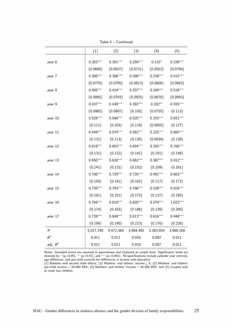
Table 4 – Continued
(1) (2) (3) (4) (5)
year 6 0.283∗∗∗ 0.301∗∗∗ 0.259∗∗∗ 0.133∗ 0.339∗∗∗
(0.0689) (0.0637) (0.0731) (0.0552) (0.0798)
year 7 0.366∗∗∗ 0.386∗∗∗ 0.306∗∗∗ 0.239∗∗∗ 0.415∗∗∗
(0.0770) (0.0705) (0.0813) (0.0606) (0.0883)
year 8 0.405∗∗∗ 0.419∗∗∗ 0.337∗∗∗ 0.249∗∗∗ 0.518∗∗∗
(0.0865) (0.0793) (0.0925) (0.0670) (0.0993)
year 9 0.437∗∗∗ 0.438∗∗∗ 0.392∗∗∗ 0.202∗∗ 0.555∗∗∗
(0.0985) (0.0907) (0.105) (0.0755) (0.113)
year 10 0.529∗∗∗ 0.548∗∗∗ 0.525∗∗∗ 0.315∗∗∗ 0.651∗∗∗
(0.111) (0.103) (0.119) (0.0855) (0.127)
year 11 0.549∗∗∗ 0.574∗∗∗ 0.582∗∗∗ 0.325∗∗∗ 0.665∗∗∗
(0.121) (0.113) (0.130) (0.0934) (0.138)
year 12 0.619∗∗∗ 0.603∗∗∗ 0.654∗∗∗ 0.355∗∗∗ 0.768∗∗∗
(0.131) (0.122) (0.141) (0.101) (0.149)
year 13 0.650∗∗∗ 0.630∗∗∗ 0.662∗∗∗ 0.387∗∗∗ 0.812∗∗∗
(0.141) (0.131) (0.152) (0.109) (0.161)
year 14 0.706∗∗∗ 0.729∗∗∗ 0.720∗∗∗ 0.491∗∗∗ 0.863∗∗∗
(0.150) (0.141) (0.162) (0.117) (0.172)
year 15 0.739∗∗∗ 0.793∗∗∗ 0.796∗∗∗ 0.539∗∗∗ 0.924∗∗∗
(0.161) (0.151) (0.173) (0.127) (0.185)
year 16 0.769∗∗∗ 0.810∗∗∗ 0.820∗∗∗ 0.574∗∗∗ 1.023∗∗∗
(0.174) (0.163) (0.186) (0.139) (0.200)
year 17 0.739∗∗∗ 0.849∗∗∗ 0.813∗∗∗ 0.616∗∗∗ 0.948∗∗∗
(0.198) (0.190) (0.213) (0.170) (0.228)
N 5,017,248 4,472,364 3,984,492 3,363,924 3,966,168
R2 0.011 0.011 0.010 0.007 0.011
adj. R2 0.011 0.011 0.010 0.007 0.011
Notes: Standard errors are reported in parentheses and clustered at couple level. Significance levels aredenoted by ∗ (p<0.05), ∗∗ (p<0.01), and ∗∗∗ (p<0.001). All specifications include calender year controls,age difference, and pre-child controls for differences in income and education.(1) Baseline with second child effects, (2) Mothers’ and fathers’ income ¿ 0, (3) Mothers’ and fathers’pre-child income > 50,000 SEK, (4) Mothers’ and fathers’ income > 50,000 SEK, and (5) Couples withat most two children
IFAU – Gender differences in sickness absence and the gender division of family responsibilities 25
Finally and most importantly, the long-term yearly effects of parenthood are of the
same magnitude whether we control for second-child pregnancy and second-child year 1
and 2 effects (first column of Table 4), or not (third column of Table 3). To further push
this point, we have estimated the specification with second-child controls for the sub-
sample of couples that get at most two children (fifth column of Table 4). The results are
qualitatively unchanged, but the long-term estimates are even somewhat higher for this
group. This is an important result as it implies that the long-term results of parenthood
that we estimate are not driven by later pregnancies.
5.2.2 Composition of sickness benefit eligible individuals
In order to investigate whether a potential change in the composition of individuals el-
igible for sickness benefit after entering parenthood may affect the results, we have re-
estimated the model on a sample in which we require a positive income also after the
arrival of the first child. The estimated effects are virtually the same with and without
this additional restriction (see columns 1 and 2 in Table 4), undoubtedly due to the fact
that most individuals in Sweden stay in the labour force also after they have entered par-
enthood. Furthermore, making the pre-child labour market attachment condition more
restrictive than in the baseline sample (incomes greater than 50,000 SEK, or approxi-
mately 4,500 EUR, two years before child birth)19, implies a loss of about one million
observations, but no significant change in the results (see column 3 in Table 4). Finally,
when we make the restriction even harder so that the incomes of both parents must be
above 50,000 SEK both before and after child birth, the long-term effects are smaller (see
column 4 in Table 4), but the effect for year 15 is still as much as 0.54 sick days/month.
6 Family responsibilities and sickness absenceIn this section we discuss and investigate possible explanations for the gender differences
in sickness absence usage after parenthood observed in the previous section. We have
two ideas. The first focuses on women’s dual responsibility associated with parenthood,
which may cause either a relative deterioration in female health (cf. Bratberg et al., 2002)
19The amounts are expressed in year 2008 prices.
26 IFAU – Gender differences in sickness absence and the gender division of family responsibilities
or an improvement in health (cf. Paringer, 1983). The second concerns changes in eco-
nomic incentives within the household. We first discuss these ideas and then present the
empirical results.
6.1 A gender differential change in health
Bratberg et al. (2002) claim that the gender gap in sickness absence stems from the
psychological pressure of the dual role of women, the so called “double burden”. As
the average total time spent on working is the same for men and women (SCB, 2009),
we believe that this hypothesis should not be interpreted as an effect from a higher work
load of the women on average, but rather as a potential effect from psychological strain
of switching between roles.20 The role strain theory argues that having multiple roles is
detrimental for an individual’s health and may thus increase sickness absence.21 Thus,
according to this hypothesis, women’s health would deteriorate after entering parenthood.
However, the dual role could also lead to improved health among women. Paringer
(1983) suggests that, due to women’s dual role, female health is likely to be more impor-
tant for the household than male health, since female illness does not only include forgone
earnings, but also creates an additional cost in terms of lost home production (Paringer,
1983). In this setting, it may be rational for the household to be more precautious in case
of a negative female health shock by increasing female work absence more than for a
similar male health shock, or in other words: to be more risk averse when it comes to
her health then his. According to Paringer’s hypothesis, we would observe an increased
female-male gap in sickness absence, but a long-term improvement in women’s health.
To investigate how well these empirical predictions correspond to empirical outcomes,
we apply the same empirical strategy as in the previous analysis, but instead of sickness
absence as outcome variable, we directly focus on the effect on health by analysing in-
hospital care data.
20The similarity in total time worked corresponds well with statistics from time use studies in USA, Germanyand the Netherlands (Burda et al., 2008).
21There is also a large literature theorizing on benefits of multiple roles (the role enhancement theory), as itmight make an individual feel that his or her life is more meaningful. This effect would, hence, work inthe other direction, namely improving individual health. For more discussion about multiples roles and itsimplications, see the literature review in, e.g., Mastekaasa et al. (2000).
IFAU – Gender differences in sickness absence and the gender division of family responsibilities 27
6.2 Economic incentives
It is well known that insurance coverage may change individual behaviour. Due to asym-
metric information about employee health, the sickness insurance system (with high re-
placement rates) can be used as a way of adjusting employees’ working time (cf. Allen,
1981 and Johansson and Palme, 1996). Individuals can use sickness absence as a way
of increasing their leisure time so that their real wage equals their marginal value of
leisure.22 The starting point in this paper is that parenthood implies a new inevitable
time-consuming task at home. A response to this new home commitment could be to
reduce female labour supply as many women do. However, another way of reducing the
labour working time is to increase the time on sickness benefits. We denote this potential
effect an ex ante moral hazard effect.
In comparison to low-income mothers, high-income mothers have most likely better
opportunities to deal with the new commitment at home. They have more opportunities
to adjust their contracted labour supply, to buy household goods on the market, and to
employ flexible working hours and to telework. Thus, it is reasonable to assume that low-
income mothers have stronger incentives to increase their time on sickness benefits than
high-income mothers. An informal test of this ex ante moral hazard behaviour is thus
given by studying whether the magnitude of the effect of parenthood varies with mothers’
pre-birth income level. A negative relationship between pre-birth income and the effect
of parenthood on the sickness absence gender gap provides evidence that our main effect
is partly driven by ex ante moral hazard among mothers.
Economic theory together with empirical evidence tells us that ex post moral hazard
is important in the Swedish sickness insurance system (see e.g. Johansson and Palme,
2005). That is, sickness absence decreases with the cost of being absent. When women
reduce their working time after parenthood, the cost of being absent may be reduced. For
high-income women there may be a direct effect but there is also, most likely, a more
important indirect effect. The direct effect stems from the fact that there is a cap in the
sickness insurance system. For women with incomes above the cap, the income loss in
case of sickness absence is lower than the nominal replacement rate in the insurance.22Real wage = (income + benefits)/(contracted working hours - time on sickness benefits)
28 IFAU – Gender differences in sickness absence and the gender division of family responsibilities
Consequently, a reduction in working time for these women implies an increase in real
replacement rates. The indirect effect stems from a change in employers’ expectations
about worker performance due to the reduction in working time. High presence at work
is most likely taken as a signal of aspiration and productivity by most employers. Thus,
work absence as measured by sickness absence and/or a reduction of working time due
to household work might negatively affect future advancements at the workplace. Less
opportunities and possibilities of advancement will most likely affect work incentives,
which in turn lower the threshold for using the sickness insurance. Seen from this per-
spective, the fact that many women reduce their labour supply after entering parenthood
means that their cost of being absent falls with their lower labour market attachment.
We investigate the hypothesis of ex post moral hazard behaviour due to a change in
female labour market attachment after parenthood by studying whether a higher income
increase between year j =−2 and year j = s−1 is related to a lower effect of parenthood
on sickness absence during year s. By using lagged income as a measurement of labour
supply, we mitigate the obvious measurement problem, namely that there is a mechanical
relation between labour income23 and the number of days absent due to sickness.
6.3 Empirical results
6.3.1 Health
In order to investigate whether there is a negative health effect of family formation on
the gender gap in health, we use in-hospital care data. As we have hospitalization data
for a shorter period of time (1987 to 2005 instead of 1986 to 2008 as is the case of
sickness absence), we re-estimate, for the sake of comparison, the effect on sickness
absence for this shorter period. A comparison between the results for hospitalization
and sickness absence is presented in Table 5. The empirical specification and population
is the same as in column 5 in Table 4 (couples with at most two children), but there are
fewer observations because of the shorter period. The results on sickness absence are
very similar to the ones presented previously for the longer time period (cf. column 5 in
Table 4 and column 2 in Table 5). Furthermore, as expected, there is a substantial increase
23We measure labour supply as labour income since we lack an appropriate measure on labour supply in termsof hours worked.
IFAU – Gender differences in sickness absence and the gender division of family responsibilities 29
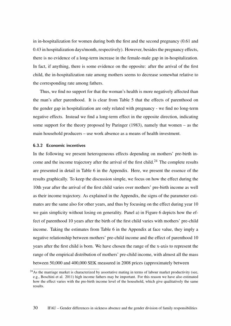
in in-hospitalization for women during both the first and the second pregnancy (0.61 and
0.43 in hospitalization days/month, respectively). However, besides the pregnancy effects,
there is no evidence of a long-term increase in the female-male gap in in-hospitalization.
In fact, if anything, there is some evidence on the opposite: after the arrival of the first
child, the in-hospitalization rate among mothers seems to decrease somewhat relative to
the corresponding rate among fathers.
Thus, we find no support for that the woman’s health is more negatively affected than
the man’s after parenthood. It is clear from Table 5 that the effects of parenthood on
the gender gap in hospitalization are only related with pregnancy - we find no long-term
negative effects. Instead we find a long-term effect in the opposite direction, indicating
some support for the theory proposed by Paringer (1983), namely that women – as the
main household producers – use work absence as a means of health investment.
6.3.2 Economic incentives
In the following we present heterogeneous effects depending on mothers’ pre-birth in-
come and the income trajectory after the arrival of the first child.24 The complete results
are presented in detail in Table 6 in the Appendix. Here, we present the essence of the
results graphically. To keep the discussion simple, we focus on how the effect during the
10th year after the arrival of the first child varies over mothers’ pre-birth income as well
as their income trajectory. As explained in the Appendix, the signs of the parameter esti-
mates are the same also for other years, and thus by focusing on the effect during year 10
we gain simplicity without losing on generality. Panel a) in Figure 6 depicts how the ef-
fect of parenthood 10 years after the birth of the first child varies with mothers’ pre-child
income. Taking the estimates from Table 6 in the Appendix at face value, they imply a
negative relationship between mothers’ pre-child income and the effect of parenthood 10
years after the first child is born. We have chosen the range of the x-axis to represent the
range of the empirical distribution of mothers’ pre-child income, with almost all the mass
between 50,000 and 400,000 SEK measured in 2008 prices (approximately between
24As the marriage market is characterized by assortative mating in terms of labour market productivity (see,e.g., Boschini et al. 2011) high income fathers may be important. For this reason we have also estimatedhow the effect varies with the pre-birth income level of the household, which give qualitatively the sameresults.
30 IFAU – Gender differences in sickness absence and the gender division of family responsibilities
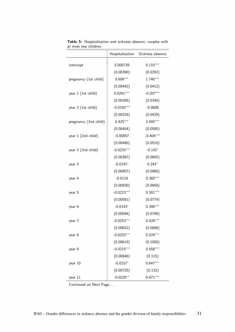
Table 5: Hospitalization and sickness absence, couples withat most two children.
Hospitalization Sickness absence
intercept 0.000739 0.110∗∗∗
(0.00390) (0.0292)
pregnancy (1st child) 0.609∗∗∗ 1.740∗∗∗
(0.00442) (0.0412)
year 1 (1st child) 0.0241∗∗∗ -0.207∗∗∗
(0.00395) (0.0340)
year 2 (1st child) -0.0192∗∗∗ -0.0688
(0.00328) (0.0429)
pregnancy (2nd child) 0.425∗∗∗ 2.045∗∗∗
(0.00454) (0.0580)
year 1 (2nd child) -0.00857 -0.404∗∗∗
(0.00480) (0.0510)
year 2 (2nd child) -0.0225∗∗∗ -0.142∗
(0.00387) (0.0605)
year 3 -0.0191∗ 0.243∗
(0.00957) (0.0980)
year 4 -0.0118 0.360∗∗∗
(0.00930) (0.0958)
year 5 -0.0223∗∗∗ 0.301∗∗∗
(0.00581) (0.0774)
year 6 -0.0143∗ 0.346∗∗∗
(0.00594) (0.0799)
year 7 -0.0253∗∗∗ 0.428∗∗∗
(0.00652) (0.0886)
year 8 -0.0253∗∗∗ 0.524∗∗∗
(0.00619) (0.1000)
year 9 -0.0215∗∗∗ 0.558∗∗∗
(0.00646) (0.115)
year 10 -0.0157∗ 0.647∗∗∗
(0.00725) (0.132)
year 11 -0.0220∗∗ 0.671∗∗∗
Continued on Next Page. . .
IFAU – Gender differences in sickness absence and the gender division of family responsibilities 31
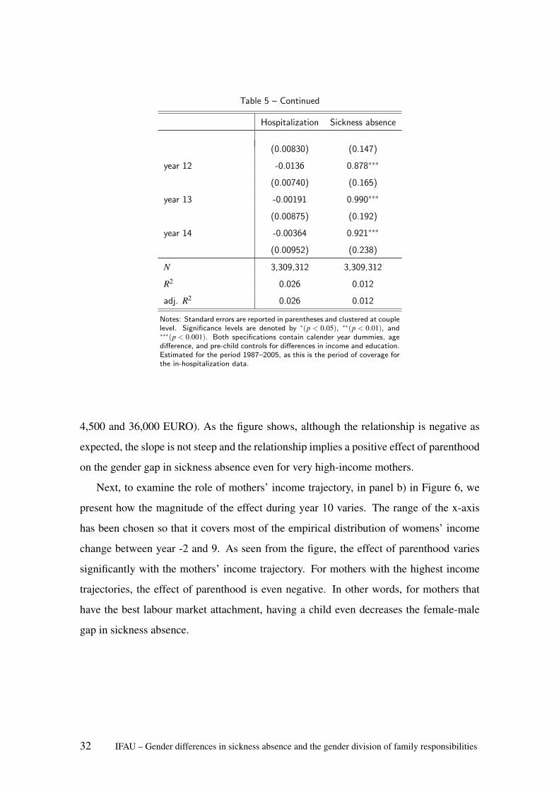
Table 5 – Continued
Hospitalization Sickness absence
(0.00830) (0.147)
year 12 -0.0136 0.878∗∗∗
(0.00740) (0.165)
year 13 -0.00191 0.990∗∗∗
(0.00875) (0.192)
year 14 -0.00364 0.921∗∗∗
(0.00952) (0.238)
N 3,309,312 3,309,312
R2 0.026 0.012
adj. R2 0.026 0.012
Notes: Standard errors are reported in parentheses and clustered at couplelevel. Significance levels are denoted by ∗(p < 0.05), ∗∗(p < 0.01), and∗∗∗(p < 0.001). Both specifications contain calender year dummies, agedifference, and pre-child controls for differences in income and education.Estimated for the period 1987–2005, as this is the period of coverage forthe in-hospitalization data.
4,500 and 36,000 EURO). As the figure shows, although the relationship is negative as
expected, the slope is not steep and the relationship implies a positive effect of parenthood
on the gender gap in sickness absence even for very high-income mothers.
Next, to examine the role of mothers’ income trajectory, in panel b) in Figure 6, we
present how the magnitude of the effect during year 10 varies. The range of the x-axis
has been chosen so that it covers most of the empirical distribution of womens’ income
change between year -2 and 9. As seen from the figure, the effect of parenthood varies
significantly with the mothers’ income trajectory. For mothers with the highest income
trajectories, the effect of parenthood is even negative. In other words, for mothers that
have the best labour market attachment, having a child even decreases the female-male
gap in sickness absence.
32 IFAU – Gender differences in sickness absence and the gender division of family responsibilities
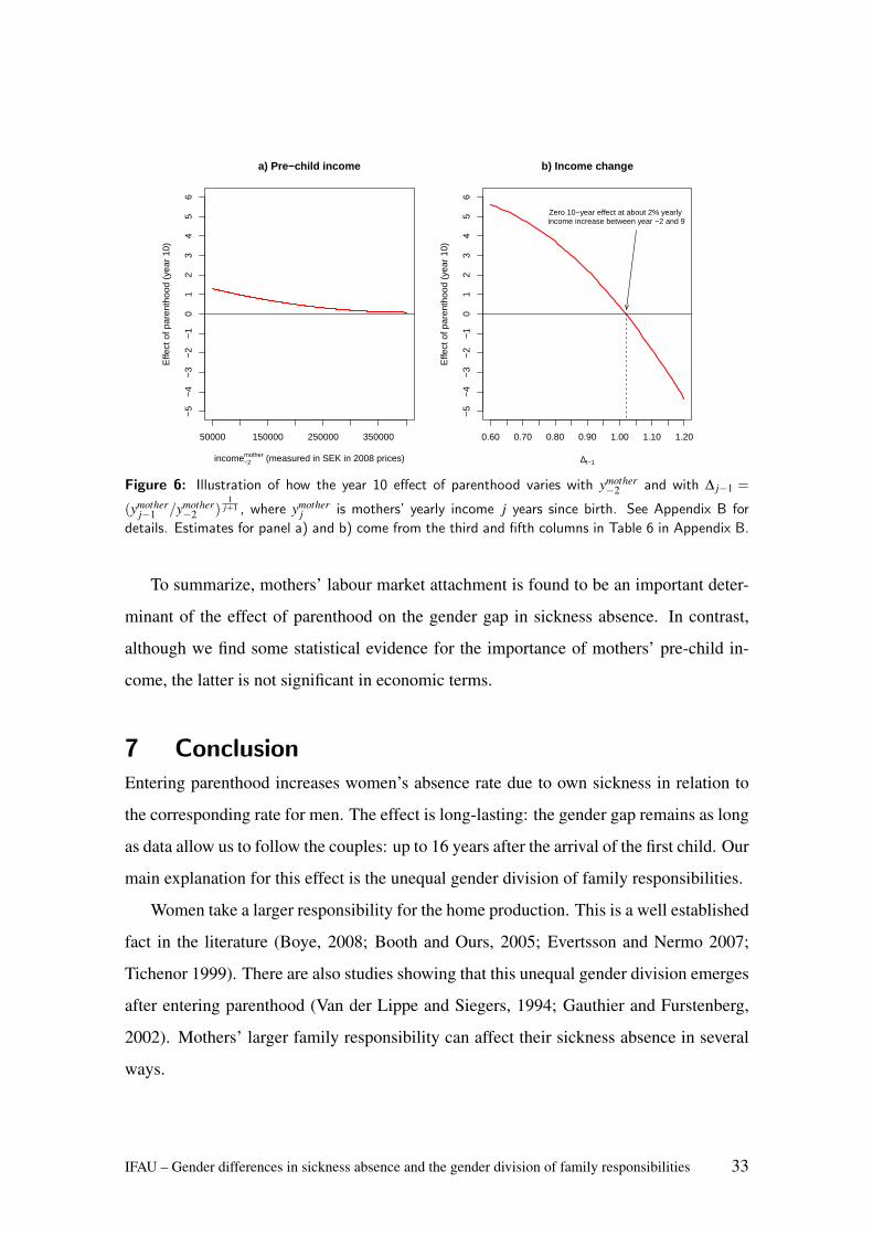
a) Pre−child income
income−2mother (measured in SEK in 2008 prices)
Effe
ct o
f par
enth
ood
(yea
r 10
)
50000 150000 250000 350000
−5
−4
−3
−2
−1
01
23
45
6
b) Income change
∆t−1
Effe
ct o
f par
enth
ood
(yea
r 10
)0.60 0.70 0.80 0.90 1.00 1.10 1.20
−5
−4
−3
−2
−1
01
23
45
6
Zero 10−year effect at about 2% yearly income increase between year −2 and 9
Figure 6: Illustration of how the year 10 effect of parenthood varies with ymother−2 and with ∆ j−1 =
(ymotherj−1 /ymother
−2 )1
j+1 , where ymotherj is mothers’ yearly income j years since birth. See Appendix B for
details. Estimates for panel a) and b) come from the third and fifth columns in Table 6 in Appendix B.
To summarize, mothers’ labour market attachment is found to be an important deter-
minant of the effect of parenthood on the gender gap in sickness absence. In contrast,
although we find some statistical evidence for the importance of mothers’ pre-child in-
come, the latter is not significant in economic terms.
7 ConclusionEntering parenthood increases women’s absence rate due to own sickness in relation to
the corresponding rate for men. The effect is long-lasting: the gender gap remains as long
as data allow us to follow the couples: up to 16 years after the arrival of the first child. Our
main explanation for this effect is the unequal gender division of family responsibilities.
Women take a larger responsibility for the home production. This is a well established
fact in the literature (Boye, 2008; Booth and Ours, 2005; Evertsson and Nermo 2007;
Tichenor 1999). There are also studies showing that this unequal gender division emerges
after entering parenthood (Van der Lippe and Siegers, 1994; Gauthier and Furstenberg,
2002). Mothers’ larger family responsibility can affect their sickness absence in several
ways.
IFAU – Gender differences in sickness absence and the gender division of family responsibilities 33
We find no support for health deterioration among women after entering parenthood.
Indeed, we find some evidence on the opposite, namely that in the long run, mothers’
in-hospitalization rate decreases somewhat relative to that of fathers. This result supports
the idea of Paringer, namely that households invest in the health of the main household
producer. This is also in line with the fact that women outlive men. During the last 30
years, the gender gap in longevity has decreased in Sweden.25 An explanation could be a
more equal gender division of household work and labour market work between men and
women.26
We find some weak evidence that the effect of parenthood on sickness absence varies
across women with different pre-birth incomes. This result supports the idea that women
with different economic situations face different opportunities to reconcile the home-
commitment and continue to work on the labour market and thereby face different in-
centives for using the sickness insurance.
Most significant for the magnitude of the effect is the female income trajectory since
birth. Many mothers change their intensive-margin labour supply due to parenthood, par-
ticularly in Sweden where a lower labour supply among parents is indirectly encouraged
by the flexible and generous Swedish parental leave system. We find that mothers’ in-
come trajectory since giving birth is strongly related to the magnitude of the effect; the
less favourable income trajectory, the more absent due to sickness. Mothers’ labour sup-
ply is measured one year prior to sickness absence, and thus this result suggests that the
lower labour supply induces more absence due to sickness rather than the other way round.
Our interpretation of this result is that a lower labour supply induces a lower threshold for
using the sickness insurance.
Finally, when entering parenthood, women fare worse in terms of labour market out-
comes. However, women’s choices, including higher sickness absence, might pay-off in
health as suggested by Paringer (1983).27
25According to data from Statistics Sweden:http://www.scb.se/Pages/Article____333965.aspx.
26Survey data on the gender division of household work during the last 20 years support this idea to someextent. Also, men have increased their parental leave over time. Both observations could be seen as anindicator of a more equal gender division of the time spent on labour market work and household work.
27See also Lee (2010) for a discussion of gender differences in health related behaviour.
34 IFAU – Gender differences in sickness absence and the gender division of family responsibilities
ReferencesAllen, S.G. (1981). “An empirical model of work attendance”, Review of Economics and
Statistics 63(1), pp. 77-87.
Akerlind, I., K. Alexandersson, G. Hensing, M. Leijon, and P. Bjurulf (1996): “Sex differ-
ences in sickness absence in relation to parental status”, Scandinavian Journal of Public
Health, 24(1), 27-35.
Angelov, N., Johansson P., Lindahl, E. and Lindtrom, E-A. (2011) “Kvinnors and mans
sjukfranvaro”, IFAU-rapport 2011:2.
Angrist J D and Evans W N (1998) “Children and their parents’ labor supply: evidence
from exogenous variation in family size”, American Economic Review, vol 88, nr 3, s
450-477.
Arrelov, B., Edlund, C. and Goine, H. (2006) “Grindvakterna and sjukforsakringen - sam-
spel and motspel i SKA Projektet: Sjukforsakring, kulturer and attityder”. E. Palmer (ed.)
Baxter, J., Hewitt, B. and Haynes, M. (2008). “Life course transitions and housework:
Marriage, parenthood, and time on housework”, Journal of Marriage and Family, 70,
259-272.
Booth, A.L. and Van Ours, J.C. (2005) “Hours of work and gender identity: Does part-
time work make the family happier?”, CEPR Discussion Paper No 5438, London.
Boschini, A., Hakansson C., Rosen, A. and Sjogren, A. (2011) “Trading off or having it
all? Completed fertility and mid-career earnings of Swedish men and women”, Working
paper 2011:15, IFAU
Boye, K. (2008) “Happy hour? Studies on well-being and time spent on paid and unpaid
work”, Swedish Institute for Social Research Dissertation Series no. 74.
Bratberg. E, Dahl, S.A., and Risa, A.E. 2002. “The double burden - Do combinations
IFAU – Gender differences in sickness absence and the gender division of family responsibilities 35
of career and family obligations increase sickness absence among women?”, European
Sociological Review, 18, 233-249.
Brostrom, G., P. Johansson, and M. Palme (2004) “Economic Incentives and Gender Dif-
ferences in Work Absence Behavior”, Swedish Economic Policy Review, 11, 33-63.
Burda, Michael, Daniel Hamermesh, and Philippe Weil. 2008. “The Distribution of Total
Work in the EU and US.”In Working Hours and Job Sharing in the EU and USA: Are Eu-
ropeans Lazy? Or Americans Crazy?, edited by Tito Boeri, Michael Burda, and Francis
Kramarz. Oxford: Oxford University Press
Englund, L. (2001) “Forandringar i distriktslakarnas sjukskrivningspraxis mellan aren
1996 and 2001 i ett svenskt landsting”. Falun: Centrum for Klinisk Forskning Dalarna.
Engstrom P, Hesselius, P. and Persson, M. (2007), “Excess use of Temporary Parental
Benefit”, Working Paper 2007:18, IFAU.
Evertsson, M. and Nermo, M. (2007) “Changing Resources and the Division of House-
work: A Longitudinal Study of Swedish Couples”, European Sociological Review, 23:
455-470.
Forsakringskassan (2011) Socialforsakringen i siffror 2011 (in Swedish).
Gauthier, A. and Furstenberg, F.F. Jr. (2002) “The transition to adulthood: a time use per-
spective”, The Annals of the American Academy of Political and Social Science March:
153-171
Gjerdingen, D. K. and Center, B. A. (2005). “First-time parents’ postpartum changes
in employment, childcare, and housework responsibilities”, Social Science Research, 34,
103-116.
Hedborg, A. (2012) “Under hoga tak ryms alla - en rapport om hojda tak i sjukforsakrin-
gen”, Kommunal produktion 2012.
36 IFAU – Gender differences in sickness absence and the gender division of family responsibilities
Jacobsen J P, Wishart Pierce J and Rosenbloom J L (1999) “The effects of child-bearing
on married women’s labor supply and earnings”Journal of Human Resources, vol. 34, nr
3, s 449-474
Johansson, P. and M. Palme (1996). “Do Economic Incentives Affect Work Absence?
Empirical Evidence Using Swedish Micro Data”, Journal of Public Economics, 59, s.
195-218.
Johansson, P. and Palme, M. (2005) “Moral hazard and sickness insurance”, Journal of
Public Economics, vol 89, s 1879-1890
Kennerberg, L. (2007) “Hur forandras kvinnors and mans arbetssituation nar de far barn?”,
IFAU-rapport 2007:9. Institutet for arbetsmarknads- and utbildningspolitisk utvardering,
Uppsala.
Lee, C. (2010) “Gender, Health, and Health Behaviors”, Ch. 20 in Chrisler, J.C. and Mc-
Creary D.R. (eds.), Handbook of Gender Research in Psychology, Springer Science.
Mastekaasa, A., and K. Olsen (2000): “Do women or Men have Less Healthy Jobs? An
Analysis of Gender Differences in Sickness Absence”, European Sociological Review,
16(3), 267 86.
Mastekaasa, A., and K. Olsen (1998): “Gender, Absenteeism and Job Characteristics: A
Fixed Effects Approach”, Work and Occupations, 25, 195- 2228.
Nathanson, C. (1975) “Illness and the feminine role: a theoretical review”, Social science
and medicine, vol 9, 57-62.
OECD (2010), “Gender Brief”, OECD Social Policy Division.
OECD 2004 Employment Outlook 2004.
Paringer, (1983) “Women and Absenteeism: Health or Economics”, American Economic
Review, Vol. 73, No. 2, pp. 123-127
IFAU – Gender differences in sickness absence and the gender division of family responsibilities 37
Persson, M (2011) “Substitution between temporary parental leave and sickness absence”,
Working Paper 2011:19 IFAU.
Sanchez, L. and Thomson, E. (1997). “Becoming mothers and fathers: Parenthood, gen-
der, and the division of labor”, Gender and Society, 11, 747-772.
SCB (2009) “Tid for vardagsliv – Kvinnors and mans tidsanvandning 1990/91 and 2000/01”,
Levnadsforhallanden, rapport 99 Statistiska centralbyran.
Selin, H. (2009) “The Rise in Female Employment and the Role of Tax Incentives. An
Empirical Analysis of the Swedish Individual Tax Reform of 1971”, UCFS Working Pa-
per 2009:3.
SFS. Svensk forfattningssamling: Foraldraledighetslagen 1995:584.1995:584
Sindelar, Jody L. “”Differential Use of Medical Care by Sex.”, J.P.E. 90 (October 1982):
1003-19.
SOU (2004): Den konsuppdelade arbetsmarknaden, Statens offentliga utredningar(SOU).
Stockholm 2004:43.
The World Factbook (2012) Washington, DC: Central Intelligence Agency, 2012, ac-
cessed on February 18, 2013 from https://www.cia.gov/library/publications/
the-world-factbook/index.html
Tichenor, V.J. (1999) “Status and Income as Gendered Resources: The Case of Marital
Power”, Journal of Marriage and Family, 61 638-650
U.S. Bureau of Labor Statistics (2011) “Women in the Labor Force: a Databook ”, U.S.
Department of Labor, Report 1034, December 2011
Van der Lippe, T. and Siegers, J. (1994) “Division of Household and Paid Labor between
Partners: Effects of Relative Wage Rates and Social Norms”, Kyklos, 47: 109-136.
Verbrugge, L. (1982) “Sex Differentials in Health”, Public Health Report, 97, 417-437.
38 IFAU – Gender differences in sickness absence and the gender division of family responsibilities
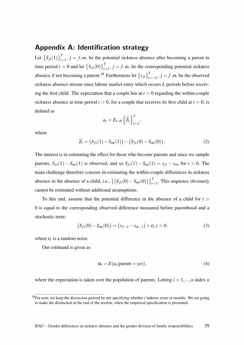
Appendix A: Identification strategy
Let{
S jt(1)}T
t=1 , j = f ,m, be the potential sickness absence after becoming a parent in
time period t = 0 and let{
S f t(0)}T
t=1 , j = f ,m, be the corresponding potential sickness
absence if not becoming a parent.28 Furthermore let{
s jt}T
t=−L , j = f ,m, be the observed
sickness absence stream since labour market entry which occurs L periods before receiv-
ing the first child. The expectation that a couple has at t = 0 regarding the within-couple
sickness absence at time period t > 0, for a couple that receives its first child at t = 0, is
defined as
at = Et=0
{Zt
}T
t=1,
where
Zt =(S f t(1)−Smt(1)
)−(S f t(0)−Smt(0)
). (2)
The interest is in estimating the effect for those who become parents and since we sample
parents, S f t(1)− Smt(1) is observed, and so S f t(1)− Smt(1) = s f t − smt for t > 0. The
main challenge therefore consists in estimating the within-couple differences in sickness
absence in the absence of a child, i.e.,{(
S f t(0)−Smt(0))}T
t=1. This sequence obviously
cannot be estimated without additional assumptions.
To this end, assume that the potential difference in the absence of a child for t >
0 is equal to the corresponding observed difference measured before parenthood and a
stochastic term: (S f t(0)−Smt(0)
)=(s f−1− sm−1
)+ εt , t > 0. (3)
where εt is a random noise.
Our estimand is given as
αt = E(at |parent = yes), (4)
where the expectation is taken over the population of parents. Letting i = 1, ...,n index n
28For now, we keep the discussion general by not specifying whether t indexes years or months. We are goingto make the distinction at the end of the section, when the empirical specification is presented.
IFAU – Gender differences in sickness absence and the gender division of family responsibilities 39
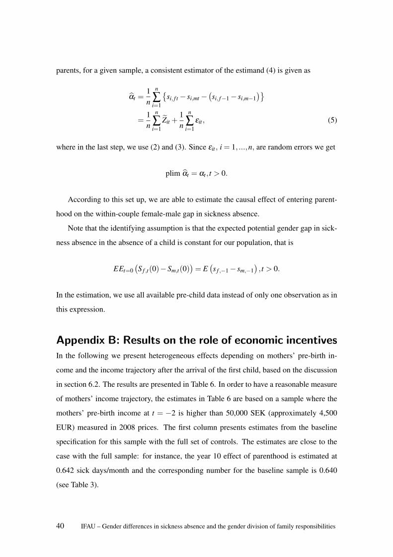
parents, for a given sample, a consistent estimator of the estimand (4) is given as
αt =1n
n
∑i=1
{si, f t− si,mt−
(si, f−1− si,m−1
)}=
1n
n
∑i=1
Zit +1n
n
∑i=1
εit , (5)
where in the last step, we use (2) and (3). Since εit , i = 1, ...,n, are random errors we get
plim αt = αt , t > 0.
According to this set up, we are able to estimate the causal effect of entering parent-
hood on the within-couple female-male gap in sickness absence.
Note that the identifying assumption is that the expected potential gender gap in sick-
ness absence in the absence of a child is constant for our population, that is
EEt=0(S f ,t(0)−Sm,t(0)
)= E
(s f ,−1− sm,−1
), t > 0.
In the estimation, we use all available pre-child data instead of only one observation as in
this expression.
Appendix B: Results on the role of economic incentivesIn the following we present heterogeneous effects depending on mothers’ pre-birth in-
come and the income trajectory after the arrival of the first child, based on the discussion
in section 6.2. The results are presented in Table 6. In order to have a reasonable measure
of mothers’ income trajectory, the estimates in Table 6 are based on a sample where the
mothers’ pre-birth income at t = −2 is higher than 50,000 SEK (approximately 4,500
EUR) measured in 2008 prices. The first column presents estimates from the baseline
specification for this sample with the full set of controls. The estimates are close to the
case with the full sample: for instance, the year 10 effect of parenthood is estimated at
0.642 sick days/month and the corresponding number for the baseline sample is 0.640
(see Table 3).
40 IFAU – Gender differences in sickness absence and the gender division of family responsibilities
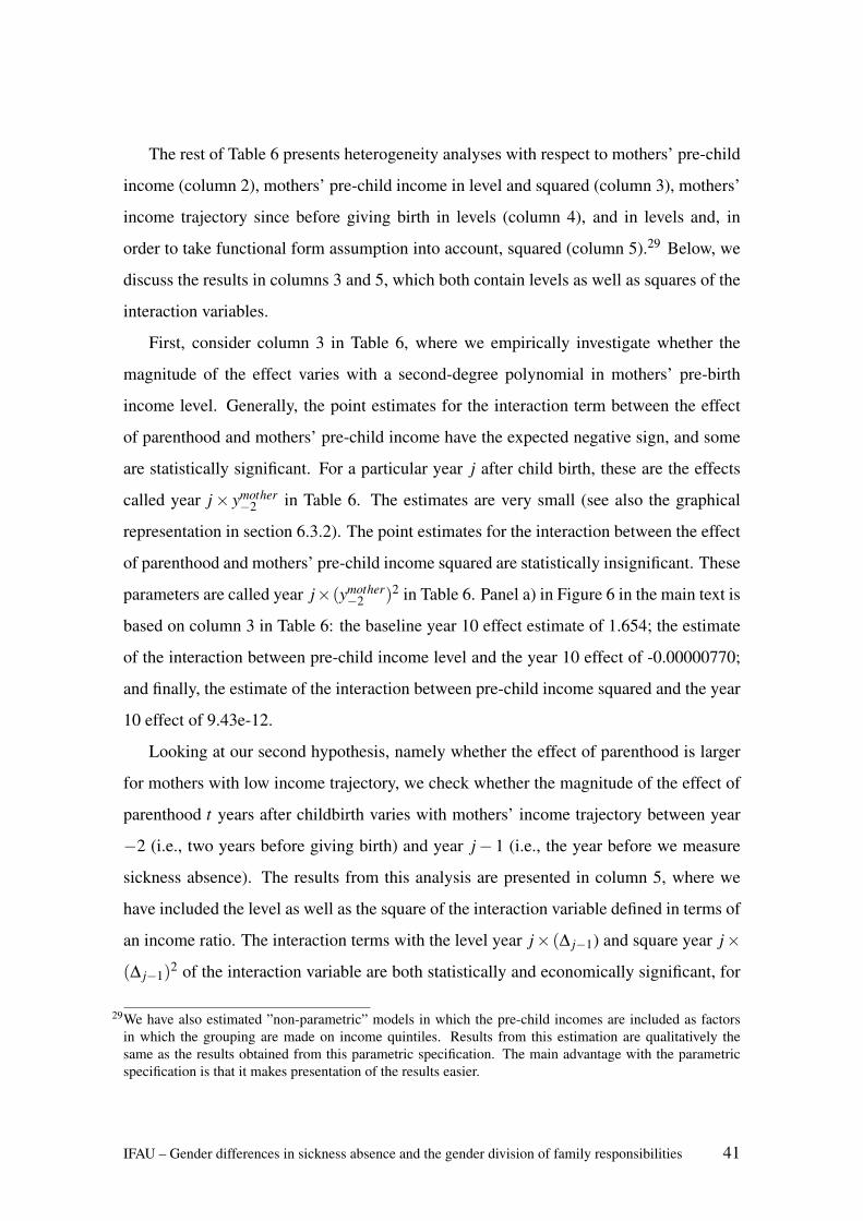
The rest of Table 6 presents heterogeneity analyses with respect to mothers’ pre-child
income (column 2), mothers’ pre-child income in level and squared (column 3), mothers’
income trajectory since before giving birth in levels (column 4), and in levels and, in
order to take functional form assumption into account, squared (column 5).29 Below, we
discuss the results in columns 3 and 5, which both contain levels as well as squares of the
interaction variables.
First, consider column 3 in Table 6, where we empirically investigate whether the
magnitude of the effect varies with a second-degree polynomial in mothers’ pre-birth
income level. Generally, the point estimates for the interaction term between the effect
of parenthood and mothers’ pre-child income have the expected negative sign, and some
are statistically significant. For a particular year j after child birth, these are the effects
called year j× ymother−2 in Table 6. The estimates are very small (see also the graphical
representation in section 6.3.2). The point estimates for the interaction between the effect
of parenthood and mothers’ pre-child income squared are statistically insignificant. These
parameters are called year j×(ymother−2 )2 in Table 6. Panel a) in Figure 6 in the main text is
based on column 3 in Table 6: the baseline year 10 effect estimate of 1.654; the estimate
of the interaction between pre-child income level and the year 10 effect of -0.00000770;
and finally, the estimate of the interaction between pre-child income squared and the year
10 effect of 9.43e-12.
Looking at our second hypothesis, namely whether the effect of parenthood is larger
for mothers with low income trajectory, we check whether the magnitude of the effect of
parenthood t years after childbirth varies with mothers’ income trajectory between year
−2 (i.e., two years before giving birth) and year j− 1 (i.e., the year before we measure
sickness absence). The results from this analysis are presented in column 5, where we
have included the level as well as the square of the interaction variable defined in terms of
an income ratio. The interaction terms with the level year j× (∆ j−1) and square year j×
(∆ j−1)2 of the interaction variable are both statistically and economically significant, for
29We have also estimated ”non-parametric” models in which the pre-child incomes are included as factorsin which the grouping are made on income quintiles. Results from this estimation are qualitatively thesame as the results obtained from this parametric specification. The main advantage with the parametricspecification is that it makes presentation of the results easier.
IFAU – Gender differences in sickness absence and the gender division of family responsibilities 41
all years. Panel b) in Figure 6 in the main text is based on column 5 in Table 6: the
baseline year 10 effect estimate of 2.562; the estimate of the interaction between ∆9 and
the year 10 effect of 15.91; and finally, the estimate of the interaction between pre-child
income squared and the year 10 effect of -18.08. The empirical distribution of ∆9 also
contains a mass at 0, i.e., women that have withdrawn from the labour force in year 9.
Those observations are used in the estimation but not shown in the figure; for ∆9, the
value of the effect is estimated at 2.562.
42 IFAU – Gender differences in sickness absence and the gender division of family responsibilities
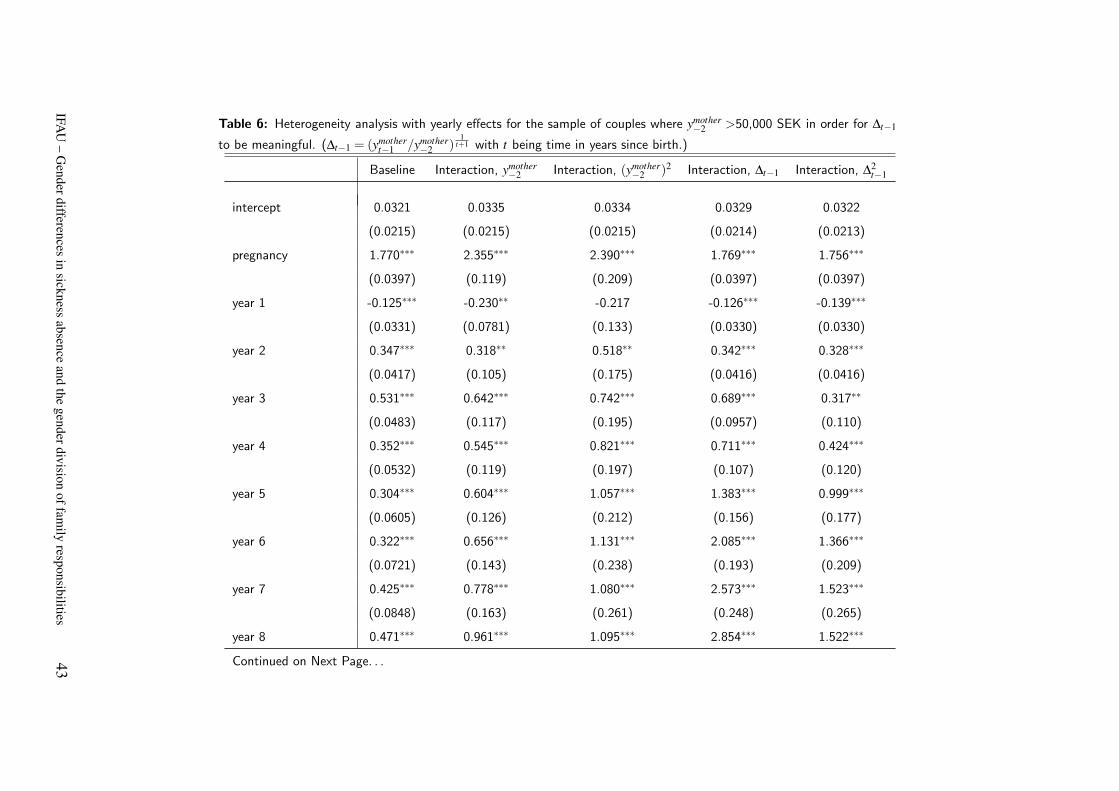
Table 6: Heterogeneity analysis with yearly effects for the sample of couples where ymother−2 >50,000 SEK in order for ∆t−1
to be meaningful. (∆t−1 = (ymothert−1 /ymother
−2 )1
t+1 with t being time in years since birth.)
Baseline Interaction, ymother−2 Interaction, (ymother
−2 )2 Interaction, ∆t−1 Interaction, ∆2t−1
intercept 0.0321 0.0335 0.0334 0.0329 0.0322
(0.0215) (0.0215) (0.0215) (0.0214) (0.0213)
pregnancy 1.770∗∗∗ 2.355∗∗∗ 2.390∗∗∗ 1.769∗∗∗ 1.756∗∗∗
(0.0397) (0.119) (0.209) (0.0397) (0.0397)
year 1 -0.125∗∗∗ -0.230∗∗ -0.217 -0.126∗∗∗ -0.139∗∗∗
(0.0331) (0.0781) (0.133) (0.0330) (0.0330)
year 2 0.347∗∗∗ 0.318∗∗ 0.518∗∗ 0.342∗∗∗ 0.328∗∗∗
(0.0417) (0.105) (0.175) (0.0416) (0.0416)
year 3 0.531∗∗∗ 0.642∗∗∗ 0.742∗∗∗ 0.689∗∗∗ 0.317∗∗
(0.0483) (0.117) (0.195) (0.0957) (0.110)
year 4 0.352∗∗∗ 0.545∗∗∗ 0.821∗∗∗ 0.711∗∗∗ 0.424∗∗∗
(0.0532) (0.119) (0.197) (0.107) (0.120)
year 5 0.304∗∗∗ 0.604∗∗∗ 1.057∗∗∗ 1.383∗∗∗ 0.999∗∗∗
(0.0605) (0.126) (0.212) (0.156) (0.177)
year 6 0.322∗∗∗ 0.656∗∗∗ 1.131∗∗∗ 2.085∗∗∗ 1.366∗∗∗
(0.0721) (0.143) (0.238) (0.193) (0.209)
year 7 0.425∗∗∗ 0.778∗∗∗ 1.080∗∗∗ 2.573∗∗∗ 1.523∗∗∗
(0.0848) (0.163) (0.261) (0.248) (0.265)
year 8 0.471∗∗∗ 0.961∗∗∗ 1.095∗∗∗ 2.854∗∗∗ 1.522∗∗∗
Continued on Next Page. . .
IFAU
–G
enderdifferencesin
sicknessabsence
andthe
genderdivisionoffam
ilyresponsibilities
43
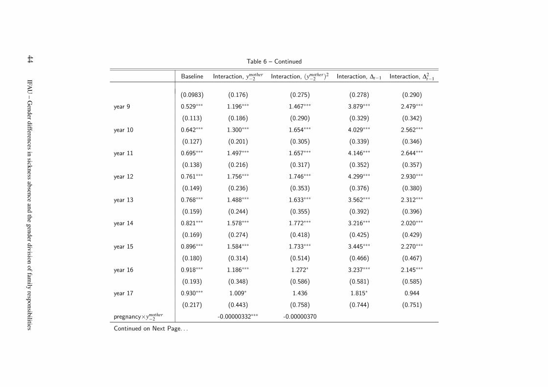
Table 6 – Continued
Baseline Interaction, ymother−2 Interaction, (ymother
−2 )2 Interaction, ∆t−1 Interaction, ∆2t−1
(0.0983) (0.176) (0.275) (0.278) (0.290)
year 9 0.529∗∗∗ 1.196∗∗∗ 1.467∗∗∗ 3.879∗∗∗ 2.479∗∗∗
(0.113) (0.186) (0.290) (0.329) (0.342)
year 10 0.642∗∗∗ 1.300∗∗∗ 1.654∗∗∗ 4.029∗∗∗ 2.562∗∗∗
(0.127) (0.201) (0.305) (0.339) (0.346)
year 11 0.695∗∗∗ 1.497∗∗∗ 1.657∗∗∗ 4.146∗∗∗ 2.644∗∗∗
(0.138) (0.216) (0.317) (0.352) (0.357)
year 12 0.761∗∗∗ 1.756∗∗∗ 1.746∗∗∗ 4.299∗∗∗ 2.930∗∗∗
(0.149) (0.236) (0.353) (0.376) (0.380)
year 13 0.768∗∗∗ 1.488∗∗∗ 1.633∗∗∗ 3.562∗∗∗ 2.312∗∗∗
(0.159) (0.244) (0.355) (0.392) (0.396)
year 14 0.821∗∗∗ 1.578∗∗∗ 1.772∗∗∗ 3.216∗∗∗ 2.020∗∗∗
(0.169) (0.274) (0.418) (0.425) (0.429)
year 15 0.896∗∗∗ 1.584∗∗∗ 1.733∗∗∗ 3.445∗∗∗ 2.270∗∗∗
(0.180) (0.314) (0.514) (0.466) (0.467)
year 16 0.918∗∗∗ 1.186∗∗∗ 1.272∗ 3.237∗∗∗ 2.145∗∗∗
(0.193) (0.348) (0.586) (0.581) (0.585)
year 17 0.930∗∗∗ 1.009∗ 1.436 1.815∗ 0.944
(0.217) (0.443) (0.758) (0.744) (0.751)
pregnancy×ymother−2 -0.00000332∗∗∗ -0.00000370
Continued on Next Page. . .
44IFA
U–
Genderdifferences
insickness
absenceand
thegenderdivision
offamily
responsibilities
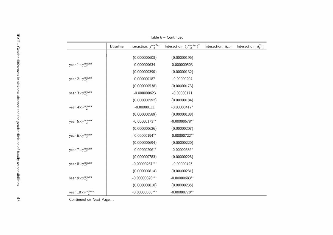
Table 6 – Continued
Baseline Interaction, ymother−2 Interaction, (ymother
−2 )2 Interaction, ∆t−1 Interaction, ∆2t−1
(0.000000608) (0.00000196)
year 1×ymother−2 0.000000634 0.000000503
(0.000000390) (0.00000132)
year 2×ymother−2 0.000000187 -0.00000204
(0.000000538) (0.00000173)
year 3×ymother−2 -0.000000623 -0.00000171
(0.000000592) (0.00000184)
year 4×ymother−2 -0.00000111 -0.00000417∗
(0.000000589) (0.00000188)
year 5×ymother−2 -0.00000173∗∗ -0.00000678∗∗
(0.000000626) (0.00000207)
year 6×ymother−2 -0.00000194∗∗ -0.00000722∗∗
(0.000000694) (0.00000220)
year 7×ymother−2 -0.00000206∗∗ -0.00000536∗
(0.000000783) (0.00000228)
year 8×ymother−2 -0.00000287∗∗∗ -0.00000425
(0.000000814) (0.00000231)
year 9×ymother−2 -0.00000390∗∗∗ -0.00000683∗∗
(0.000000810) (0.00000235)
year 10×ymother−2 -0.00000388∗∗∗ -0.00000770∗∗
Continued on Next Page. . .
IFAU
–G
enderdifferencesin
sicknessabsence
andthe
genderdivisionoffam
ilyresponsibilities
45
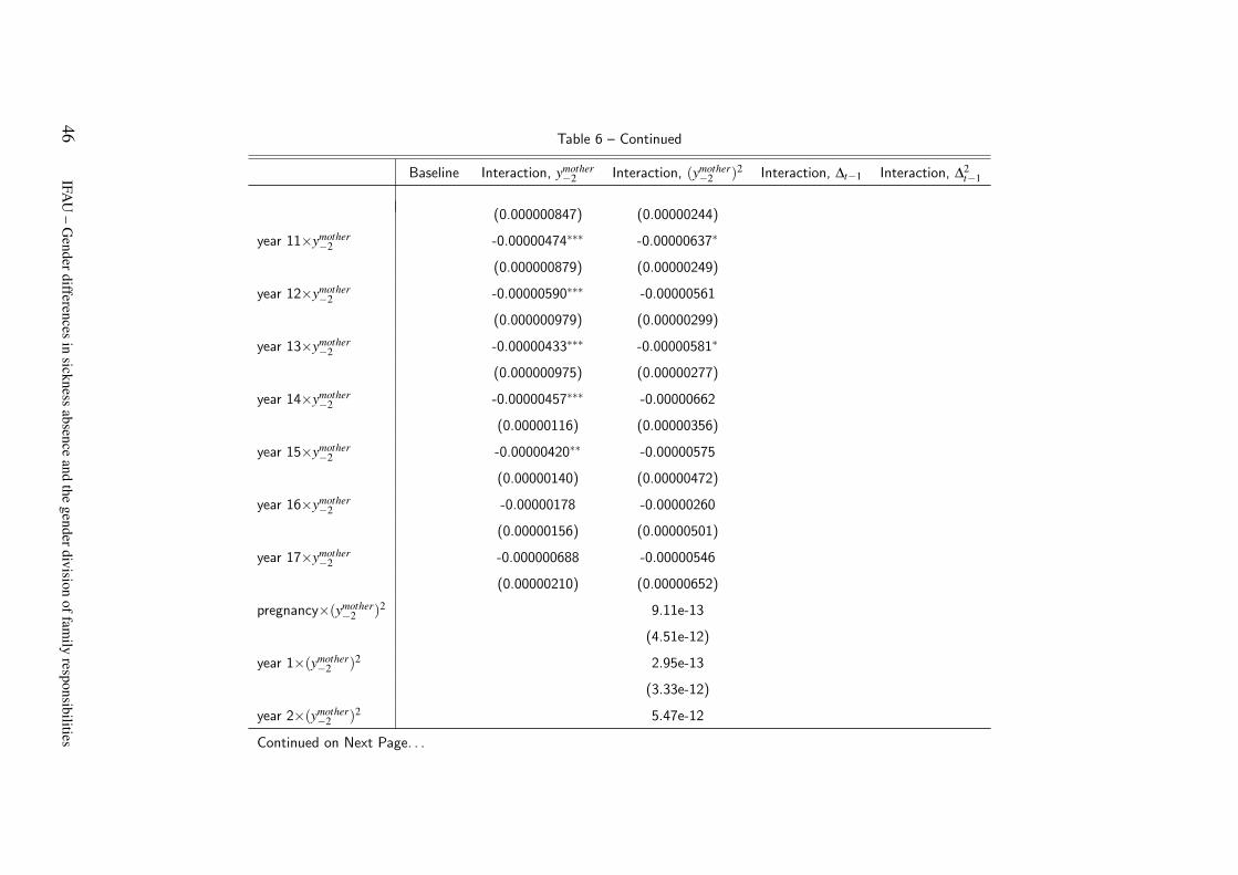
Table 6 – Continued
Baseline Interaction, ymother−2 Interaction, (ymother
−2 )2 Interaction, ∆t−1 Interaction, ∆2t−1
(0.000000847) (0.00000244)
year 11×ymother−2 -0.00000474∗∗∗ -0.00000637∗
(0.000000879) (0.00000249)
year 12×ymother−2 -0.00000590∗∗∗ -0.00000561
(0.000000979) (0.00000299)
year 13×ymother−2 -0.00000433∗∗∗ -0.00000581∗
(0.000000975) (0.00000277)
year 14×ymother−2 -0.00000457∗∗∗ -0.00000662
(0.00000116) (0.00000356)
year 15×ymother−2 -0.00000420∗∗ -0.00000575
(0.00000140) (0.00000472)
year 16×ymother−2 -0.00000178 -0.00000260
(0.00000156) (0.00000501)
year 17×ymother−2 -0.000000688 -0.00000546
(0.00000210) (0.00000652)
pregnancy×(ymother−2 )2 9.11e-13
(4.51e-12)
year 1×(ymother−2 )2 2.95e-13
(3.33e-12)
year 2×(ymother−2 )2 5.47e-12
Continued on Next Page. . .
46IFA
U–
Genderdifferences
insickness
absenceand
thegenderdivision
offamily
responsibilities
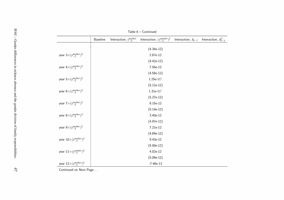
Table 6 – Continued
Baseline Interaction, ymother−2 Interaction, (ymother
−2 )2 Interaction, ∆t−1 Interaction, ∆2t−1
(4.34e-12)
year 3×(ymother−2 )2 2.67e-12
(4.42e-12)
year 4×(ymother−2 )2 7.56e-12
(4.58e-12)
year 5×(ymother−2 )2 1.25e-11∗
(5.12e-12)
year 6×(ymother−2 )2 1.31e-11∗
(5.27e-12)
year 7×(ymother−2 )2 8.15e-12
(5.14e-12)
year 8×(ymother−2 )2 3.40e-12
(4.97e-12)
year 9×(ymother−2 )2 7.21e-12
(4.69e-12)
year 10×(ymother−2 )2 9.43e-12
(5.00e-12)
year 11×(ymother−2 )2 4.02e-12
(5.09e-12)
year 12×(ymother−2 )2 -7.46e-13
Continued on Next Page. . .
IFAU
–G
enderdifferencesin
sicknessabsence
andthe
genderdivisionoffam
ilyresponsibilities
47
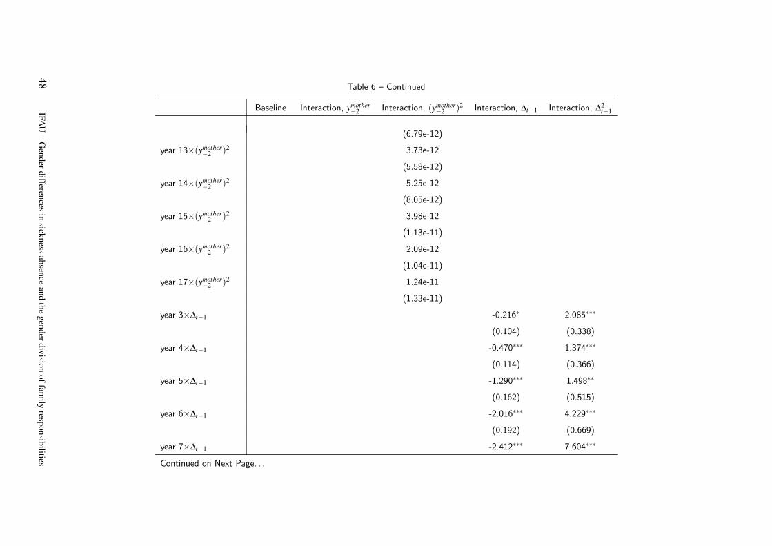
Table 6 – Continued
Baseline Interaction, ymother−2 Interaction, (ymother
−2 )2 Interaction, ∆t−1 Interaction, ∆2t−1
(6.79e-12)
year 13×(ymother−2 )2 3.73e-12
(5.58e-12)
year 14×(ymother−2 )2 5.25e-12
(8.05e-12)
year 15×(ymother−2 )2 3.98e-12
(1.13e-11)
year 16×(ymother−2 )2 2.09e-12
(1.04e-11)
year 17×(ymother−2 )2 1.24e-11
(1.33e-11)
year 3×∆t−1 -0.216∗ 2.085∗∗∗
(0.104) (0.338)
year 4×∆t−1 -0.470∗∗∗ 1.374∗∗∗
(0.114) (0.366)
year 5×∆t−1 -1.290∗∗∗ 1.498∗∗
(0.162) (0.515)
year 6×∆t−1 -2.016∗∗∗ 4.229∗∗∗
(0.192) (0.669)
year 7×∆t−1 -2.412∗∗∗ 7.604∗∗∗
Continued on Next Page. . .
48IFA
U–
Genderdifferences
insickness
absenceand
thegenderdivision
offamily
responsibilities
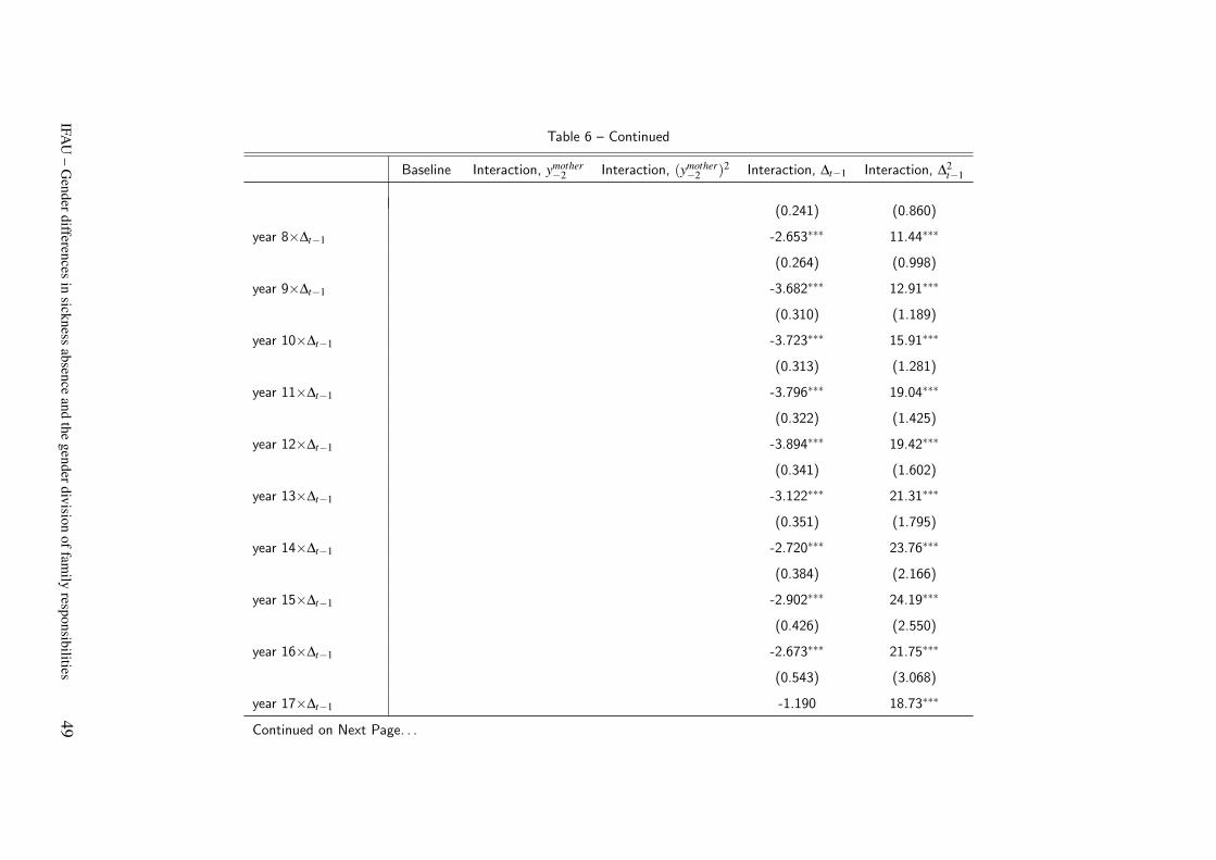
Table 6 – Continued
Baseline Interaction, ymother−2 Interaction, (ymother
−2 )2 Interaction, ∆t−1 Interaction, ∆2t−1
(0.241) (0.860)
year 8×∆t−1 -2.653∗∗∗ 11.44∗∗∗
(0.264) (0.998)
year 9×∆t−1 -3.682∗∗∗ 12.91∗∗∗
(0.310) (1.189)
year 10×∆t−1 -3.723∗∗∗ 15.91∗∗∗
(0.313) (1.281)
year 11×∆t−1 -3.796∗∗∗ 19.04∗∗∗
(0.322) (1.425)
year 12×∆t−1 -3.894∗∗∗ 19.42∗∗∗
(0.341) (1.602)
year 13×∆t−1 -3.122∗∗∗ 21.31∗∗∗
(0.351) (1.795)
year 14×∆t−1 -2.720∗∗∗ 23.76∗∗∗
(0.384) (2.166)
year 15×∆t−1 -2.902∗∗∗ 24.19∗∗∗
(0.426) (2.550)
year 16×∆t−1 -2.673∗∗∗ 21.75∗∗∗
(0.543) (3.068)
year 17×∆t−1 -1.190 18.73∗∗∗
Continued on Next Page. . .
IFAU
–G
enderdifferencesin
sicknessabsence
andthe
genderdivisionoffam
ilyresponsibilities
49
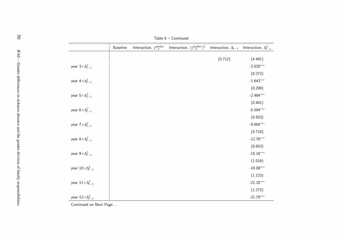
Table 6 – Continued
Baseline Interaction, ymother−2 Interaction, (ymother
−2 )2 Interaction, ∆t−1 Interaction, ∆2t−1
(0.712) (4.491)
year 3×∆2t−1 -2.020∗∗∗
(0.272)
year 4×∆2t−1 -1.643∗∗∗
(0.299)
year 5×∆2t−1 -2.484∗∗∗
(0.401)
year 6×∆2t−1 -5.594∗∗∗
(0.553)
year 7×∆2t−1 -9.004∗∗∗
(0.718)
year 8×∆2t−1 -12.76∗∗∗
(0.853)
year 9×∆2t−1 -15.16∗∗∗
(1.016)
year 10×∆2t−1 -18.08∗∗∗
(1.123)
year 11×∆2t−1 -21.20∗∗∗
(1.272)
year 12×∆2t−1 -21.79∗∗∗
Continued on Next Page. . .
50IFA
U–
Genderdifferences
insickness
absenceand
thegenderdivision
offamily
responsibilities
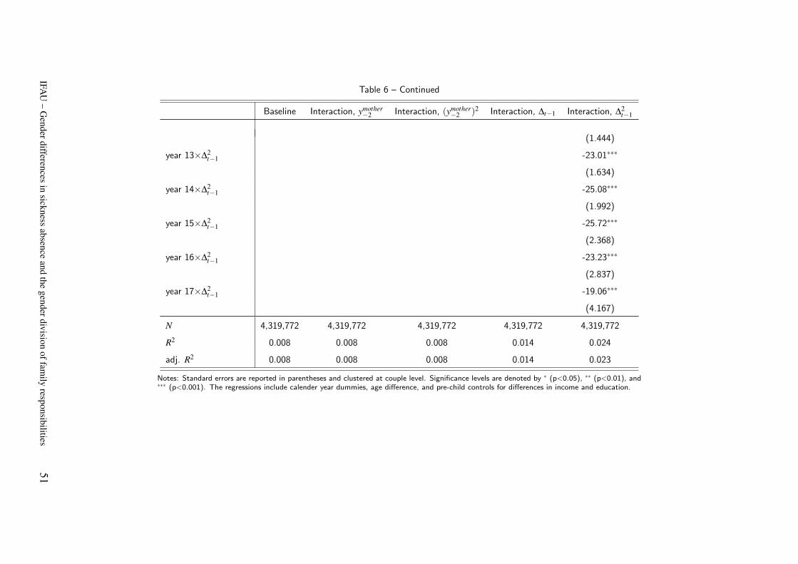
Table 6 – Continued
Baseline Interaction, ymother−2 Interaction, (ymother
−2 )2 Interaction, ∆t−1 Interaction, ∆2t−1
(1.444)
year 13×∆2t−1 -23.01∗∗∗
(1.634)
year 14×∆2t−1 -25.08∗∗∗
(1.992)
year 15×∆2t−1 -25.72∗∗∗
(2.368)
year 16×∆2t−1 -23.23∗∗∗
(2.837)
year 17×∆2t−1 -19.06∗∗∗
(4.167)
N 4,319,772 4,319,772 4,319,772 4,319,772 4,319,772
R2 0.008 0.008 0.008 0.014 0.024
adj. R2 0.008 0.008 0.008 0.014 0.023
Notes: Standard errors are reported in parentheses and clustered at couple level. Significance levels are denoted by ∗ (p<0.05), ∗∗ (p<0.01), and∗∗∗ (p<0.001). The regressions include calender year dummies, age difference, and pre-child controls for differences in income and education.
IFAU
–G
enderdifferencesin
sicknessabsence
andthe
genderdivisionoffam
ilyresponsibilities
51
Publication series published by IFAU – latest issues
Rapporter/Reports
2013:1 Olsson Martin ”Anställningsskydd och föräldrarelaterad frånvaro”
2013:2 Angelov Nikolay, Per Johansson and Erica Lindahl ”Det envisa könsgapet i inkomster och löner – Hur mycket kan förklaras av skillnader i familjeansvar?”
2013:3 Vikman Ulrika ”Så påverkar föräldraförsäkringen nyanlända invandrares etablering på arbets-marknaden”
2013:4 Forslund Anders, Linus Liljeberg and Leah von Trott zu Solz ”Arbetspraktik – en utvärdering och en jämförelse med arbetsmarknadsutbildning”
2013:5 Eliasson Tove ”Löneutveckling bland invandrade och infödda – betydelsen av arbetsplatser och yrken”
2013:6 Katz Katarina and Torun Österberg ”Unga invandrare – utbildning, löner och utbildnings-avkastning”
2013:7 Angelov Nikolay, Per Johansson and Erica Lindahl ”Kvinnors större föräldraansvar och högre sjukfrånvaro”
Working papers
2013:1 Nekby Lena, Peter Skogman Thoursie and Lars Vahtrik ”Examination behavior – Gender differences in preferences?”
2013:2 Olsson Martin “Employment protection and parental child care”
2013:3 Angelov Nikolay, Per Johansson and Erica Lindahl “Is the persistent gender gap in income and wages due to unequal family responsibilities?”
2013:4 Vikman Ulrika “Paid parental leave to immigrants: An obstacle to labor market entrance?”
2013:5 Pingel Ronnie and Ingeborg Waernbaum “Effects of correlated covariates on the efficiency of matching and inverse probability weighting estimators for causal inference”
2013:6 Forslund Anders, Linus Liljeberg and Leah von Trott zu Solz ”Job practice: an evaluation and a comparison with vocational labour market training programmes”
2013:7 Eliasson Tove “Decomposing immigrant wage assimilation – the role of workplaces and occupations”
2013:8 Katz Katarina and Torun Österberg “Wages of childhood immigrants in Sweden – education, returns to education and overeducation”
2013:9 Angelov Nikolay, Per Johansson and Erica Lindahl “Gender differences in sickness absence and the gender division of family responsibilities”
Dissertation series 2012:1 Laun Lisa “Studies on social insurance, income taxation and labor supply”


