econstor www.econstor.eu
Der Open-Access-Publikationsserver der ZBW – Leibniz-Informationszentrum WirtschaftThe Open Access Publication Server of the ZBW – Leibniz Information Centre for Economics
Standard-Nutzungsbedingungen:
Die Dokumente auf EconStor dürfen zu eigenen wissenschaftlichenZwecken und zum Privatgebrauch gespeichert und kopiert werden.
Sie dürfen die Dokumente nicht für öffentliche oder kommerzielleZwecke vervielfältigen, öffentlich ausstellen, öffentlich zugänglichmachen, vertreiben oder anderweitig nutzen.
Sofern die Verfasser die Dokumente unter Open-Content-Lizenzen(insbesondere CC-Lizenzen) zur Verfügung gestellt haben sollten,gelten abweichend von diesen Nutzungsbedingungen die in der dortgenannten Lizenz gewährten Nutzungsrechte.
Terms of use:
Documents in EconStor may be saved and copied for yourpersonal and scholarly purposes.
You are not to copy documents for public or commercialpurposes, to exhibit the documents publicly, to make thempublicly available on the internet, or to distribute or otherwiseuse the documents in public.
If the documents have been made available under an OpenContent Licence (especially Creative Commons Licences), youmay exercise further usage rights as specified in the indicatedlicence.
zbw Leibniz-Informationszentrum WirtschaftLeibniz Information Centre for Economics
Flach, Lisandra; Irlacher, Michael
Working Paper
Product versus Process: Innovation Strategies ofMulti-Product Firms
CESifo Working Paper, No. 5405
Provided in Cooperation with:Ifo Institute – Leibniz Institute for Economic Research at the University ofMunich
Suggested Citation: Flach, Lisandra; Irlacher, Michael (2015) : Product versus Process:Innovation Strategies of Multi-Product Firms, CESifo Working Paper, No. 5405
This Version is available at:http://hdl.handle.net/10419/113735

Product versus Process: Innovation Strategies of Multi-Product Firms
Lisandra Flach Michael Irlacher
CESIFO WORKING PAPER NO. 5405 CATEGORY 8: TRADE POLICY
JUNE 2015
An electronic version of the paper may be downloaded • from the SSRN website: www.SSRN.com • from the RePEc website: www.RePEc.org
• from the CESifo website: Twww.CESifo-group.org/wp T
ISSN 2364-1428
CESifo Working Paper No. 5405
Product versus Process: Innovation Strategies of Multi-Product Firms
Abstract We investigate the effect of better access to foreign markets on innovation strategies of multi-product firms in industries with different scope for product differentiation. Industry-specific demand and cost linkages induce a distinction between the returns to innovation. In differentiated industries, cannibalization is lower and firms invest more in product innovation. In homogeneous industries, firms internalize intra-firm spillovers and invest more in process innovation. We test these predictions using Brazilian firm-level data. Following an exchange rate devaluation, firms have better access to foreign markets and exploit economies of scale in innovation. We evaluate the differential effects across industries and show that the type of innovation depends on the degree of product differentiation.
JEL-Code: F120, F140, L250.
Keywords: multi-product firms, innovation, product differentiation, cannibalization effect, spillovers, market size effect.
Lisandra Flach Department of Economics
University of Munich 80539 Munich / Germany
Michael Irlacher Department of Economics
University of Munich 80539 Munich / Germany
June 15, 2015 We are grateful to Daniel Baumgarten, Carsten Eckel, Kalina Manova, Thierry Mayer, Emanuel Ornelas, Jennifer Poole, Jens Suedekum, and participants at the 16th Workshop International Economics in Goettingen 2014, European Economic Association in Toulouse, European Trade Study Group in Munich, FIW Research Conference in Vienna, Midwest International Economics Group in Columbus and IO-Trade Seminar Munich for their helpful comments. Part of this paper was written while one of the coauthors (Lisandra Flach) was visiting the Brazilian Statistical Office (IBGE), whose support and hospitality is gratefully acknowledged. Financial support from SFB TR 15 is gratefully acknowledged. Felix Roellig provided excellent research assistance.

1 Introduction
Successful manufacturing �rms continuously innovate to maintain their position in the mar-
ket and to attend consumers�demand. Recent contributions in the international trade liter-
ature emphasize the importance of intra-�rm adjustments through innovation in explaining
welfare gains from trade liberalization, besides the well-established intra-industry gains from
entry and exit of �rms. This literature highlights innovation as a new dimension into the re-
lationship between exporting and productivity: Better access to foreign markets encourages
�rms to invest in more sophisticated manufacturing technologies, which increases produc-
tivity.1 Consequently, innovation and productivity improvements within the �rm account
for a large fraction of productivity gains at the industry level.2 Moreover, variety-loving
consumers bene�t not only from new products of entering �rms but, �rst and foremost,
from product innovation by incumbent �rms.3 Therefore, understanding innovation strate-
gies and within-�rm adjustments of multi-product �rms (MPFs) is crucial for the analysis
of aggregate productivity and variety gains.
MPFs account for the majority of trade �ows and are omnipresent in all industries.
In terms of innovation activities, their investments account for a large fraction of aggregate
changes in industry-level productivity and product variety (Bernard et al. (2010), Broda and
Weinstein (2010), Lileeva and Tre�er (2010), Bustos (2011)). However, with the exception of
Dhingra (2013) (which is discussed later in detail), innovation in trade models happens only in
one dimension, whereas in reality �rms face a trade-o¤between investments in cost reduction
and product variety. This raises the question of how and why �rms in di¤erent industries
make their choices between di¤erent types of innovation, with di¤erent implications in terms
of welfare gains within industries.
The contribution of the paper is to investigate, theoretically and empirically, the inno-
vation strategies of MPFs, focusing on within-�rm adjustments. An increase in market size
increases the incentives for �rms to invest in innovation. However, demand and cost linkages
induce a trade-o¤ between product and process innovation. Crucially, such linkages are only
1Lileeva and Tre�er (2010) as well as Bustos (2011) show that following a tari¤ cut �rms increase theirinvestments in technology. Lileeva and Tre�er (2010) use tari¤ cuts associated with the US-Canadian freetrade agreement and show that Canadian �rms increased labor productivity and used more sophisticatedmanufacturing technologies. Furthermore, access to larger markets induced �rms to engage more in productinnovation. For Argentinean �rms, Bustos (2011) �nds an increase in innovation expenditures between 0.20and 0.28 log points following the average reduction in Brazil�s tari¤s.
2Doraszelski and Jaumandreu (2013) show for Spanish �rms that investments in R&D are the primarysource of productivity growth. Within sectors, between 65 percent and 90 percent of productivity growtharises through intra-�rm productivity enhancing activities.
3Recent evidence of US bar code data in Broda and Weinstein (2010) highlights the importance of thischannel. They show that at a four-year period, 82 percent of product creation happens within existing �rms.Therefore only 18 percent of total household expenditure is on products of entering �rms.
1
present in an MPF setting. Firms may decide to expand their product range or to lower
production costs, and the net e¤ect in terms of returns to innovation is a priori unclear.
In a simple model of MPFs, we show that returns to product and process innovation are
industry-speci�c and uncover a mechanism related to the degree of product di¤erentiation
that explains this relation. On the one hand, by introducing new products �rms internalize
demand linkages, which may reduce demand for its own varieties. On the other hand, as a
novel feature of our model, by investing in process innovation �rms may internalize intra-
�rm spillover e¤ects between production lines. To understand the role played by the degree
of di¤erentiation in this mechanism, consider two �rms in sectors with di¤erent scope for
product di¤erentiation. A �rm producing multiple products in a homogeneous industry has
rather low returns from investing in new products as doing so may crowd out demand for
its own products. This e¤ect is known as the �cannibalization e¤ect�in the literature. On
the other hand, investments in process-optimizing technologies may generate a larger return,
since the bene�ts from spillover e¤ects across production lines are larger. With more similar
production processes, the knowledge learned in the production process of more homogeneous
products is applicable to a large fraction on the entire product portfolio. For �rms in highly
di¤erentiated industries, the mechanism works exactly the other way round.
Our theoretical model builds on Eckel and Neary (2010) and Eckel et al. (2015). Each �rm
produces a bundle of products which are linked on the cost side by a �exible manufacturing
technology. The latter captures the idea that - besides a core competence - MPFs can expand
their portfolio with varieties that are less e¢ cient in production.4 However, our theory
introduces several novel features. First, we explicitly allow for two types of R&D. Therefore,
we assign �xed costs to additional products to model the decision on optimal scope, which
is closer to the notion of product innovation.5 Second, �rms can invest in product-speci�c
process innovation. Process innovation is costly and re�ects economies of scale, such that
�rms invest more in large-scale varieties, close to their core competence. Third, another novel
feature of our framework is to allow for spillover e¤ects between the production processes
within the �rm. We relate the strength of these cost linkages to the degree of product
di¤erentiation in a sector. This occurs because products that are closer substitutes tend to
have more similar production processes (in comparison to highly di¤erentiated products).
Our framework has important implications for understanding how �rms react to trade
openness and to changes in market size. In particular, the model provides two main testable
predictions. (1) We show that, following an increase in market size, �rms invest more in
4The idea that �rms possess a core competency is also featured in models with MPFs by Qiu and Zhou(2013), Arkolakis et al. (2014), and Mayer et al. (2014).
5In our framework, we always refer to product innovation as an increase in product scope.
2
both product and process innovation. Since process innovation re�ects economies of scale,
access to a larger market promotes technology upgrading. Furthermore, access to larger
markets reduce the perceived costs of product innovation, which encourages MPFs to extend
their product scope. (2) However, in our framework, demand and cost linkages related
to the degree of product di¤erentiation determine returns to innovation. We show that in
highly di¤erentiated industries, the cannibalization e¤ect is lower and, therefore, �rms invest
more in product innovation. In homogeneous industries, �rms internalize higher intra-�rm
spillover e¤ects and invest more in process innovation.
The predictions from the model are tested using detailed �rm-level data, which has two
distinctive features. First, we can exploit detailed information on innovation investments by
�rms, mainly over the years 1998-2000. Second, the event of a major and unexpected ex-
change rate devaluation in January 1999 provides an important source of exogenous variation.
For Brazilian exporters, the currency devaluation made their products more competitive at
home and abroad and, therefore, the shock may be interpreted as an increase in market size.
Moreover, we are interested in how �rms in di¤erent industries reacted to the exchange rate
shock, in order to test prediction (2) from the model. To tackle this issue empirically, we
use information on di¤erent types of innovation combined with the degree of di¤erentiation
of the industry.
Our empirical results reveal that �rms increased their innovation e¤orts in both product
and process innovation following the exchange rate devaluation. However, detailed infor-
mation on the degree of di¤erentiation and on the types of innovation conducted by �rms
allows us to evaluate di¤erential e¤ects across industries. Using a continuous measure of
the degree of di¤erentiation in an industry, we show that �rms in more di¤erentiated indus-
tries invest more in product innovation, while �rms in more homogeneous industries invest
more in process innovation. Our results are robust to di¤erent measures of the degree of
di¤erentiation, hold for di¤erent estimation strategies (we estimate the incidence of innova-
tion using probit, linear probability model, and seemingly unrelated regression), and remain
stable when adding several control variables.
Our paper is closely related to the literature on MPFs in international trade that features
a cannibalization e¤ect.6 Our theory builds on Eckel et al. (2015), who incorporate an
endogenous investment in product quality in the framework by Eckel and Neary (2010).
We abstract from investments in quality and instead focus on investments in product and
process innovation. The paper that is closest in spirit to ours is Dhingra (2013), who also
6Eckel and Neary (2010) and Dhingra (2013) introduce cannibalization e¤ects. However, this feature isnot considered in many recent models of MPFs that assume monopolistic competition. One exception is themodel proposed by Feenstra and Ma (2008).
3
considers an innovation trade-o¤ of MPFs. Dhingra (2013) proposes a model of MPFs with
intra-brand cannibalization that induces a distinction between the returns to product and
process innovation. Her framework explains how �rms react to trade liberalization in terms
of innovation investments. Following a trade liberalization, �rms face higher competition
from foreign �rms and, therefore, reduce investments in product innovation to mitigate
internal competition (cannibalization e¤ect). On the other hand, �rms increase investments
in process innovation because of economies of scale. In contrast to her theoretical framework,
we build a framework with demand and cost linkages to evaluate heterogeneous responses of
�rms in di¤erent industries. Moreover, using detailed �rm-level data, we test the predictions
from the model. In terms of the way we model innovation, the key di¤erences between our
paper and that of Dhingra (2013) are that we (1) allow for �exible manufacturing and (2)
introduce cost linkages related to the degree of di¤erentiation that generate spillover e¤ects
within the �rm. Therefore, our model is able to generate novel predictions regarding the two
types of innovation depending on the degree of di¤erentiation of the industry.
Our paper is also related to the literature emphasizing the complementary between mar-
ket size and innovation behavior of �rms that leads to gains from trade. Since innovation is
costly, changes in market size tend to encourage �rms to incur these costs because of scale ef-
fects. Models such as Grossman and Helpman (1991) investigate the gains from trade arising
from innovation investments in a setting with homogeneous �rms. At the �rm-level, several
papers have investigated the relation between changes in market size and innovation. Lileeva
and Tre�er (2010) investigate theoretically and empirically how changes in market size en-
couraged �rms to innovate. Using responses of Canadian plants to the elimination of U.S.
tari¤s, they �nd that plants more induced by the tari¤ cuts increase more their investments
in innovation. Yeaple (2005), Verhoogen (2008), and Aw et al. (2011) investigate further
channels that relate market size with �rm-level innovation and within-�rm adjustments.
2 The Model
Our theory draws on a simple model of MPFs that choose their optimal spending on product
and process innovation. Both types of innovation are costly and, therefore, �rms weight the
returns to innovation against the costs. The returns to innovation are in the focus of this
paper and constitute the main testable predictions from the model. First, we show that the
returns to product and process innovation are higher in a larger market. Second, we point out
that �rms in sectors with homogeneous products focus on optimizing production processes
while �rms in more di¤erentiated industries concentrate on innovating new products. These
innovation patterns follow from demand and cost linkages, both related to the degree of
4

product di¤erentiation in a sector. Since these linkages determine the returns to innovation,
we will introduce them at the very outset.
We begin with a detailed analysis of consumer behavior and the underlying preference
structure in section 2.1. In this part, we show how the demand linkages enter our framework
and relate them to the degree of product di¤erentiation in a sector. In section 2.2, we present
the �rm side of the model. We start with the production cost function, which is characterized
by �exible manufacturing. Moreover, �rms can undertake investments in process innovation
to reduce production costs of a product, which may generate spillovers between production
lines. We refer to this feature as a cost linkage and argue that its strength decreases in
the degree of product di¤erentiation. Firms consider both linkages when maximizing their
pro�ts. Finally, section 2.3 derives the equilibrium of the model and establishes the main
testable predictions from the theory.
2.1 Consumer Behavior: Preferences and Demand
Our economy consists of L consumers who maximize their utility over the consumption of
a homogeneous and a di¤erentiated good. To be more speci�c, we assume that consumers
buy a set of goods out of a potential set e of the di¤erentiated product. Our speci�cationof preferences follows Eckel et al. (2015), though we add an additional numeraire good and
assume a quasi-linear utility in the following form:7
U = q0 + u1, (1)
where q0 is the consumption of the homogeneous good. We conduct our analysis in partial
equilibrium where the outside good absorbs any income e¤ects. Utility over the di¤erentiated
variety is de�ned in a standard quadratic function as follows
u1 = aQ�1
2b
�(1� e)
Zi2e q(i)
2di+ eQ2�, (2)
where a and b represent non-negative preference parameters. In this speci�cation, q (i) de-
notes per variety consumption and Q �Ri2e q(i)di stands for total consumption of the
representative consumer. The parameter e plays a very important role in our model and
describes the degree of product di¤erentiation. We assume that e lies strictly between zero
and one and de�ne the parameter as an inverse measure for product di¤erentiation. This
means that lower values of e imply more di¤erentiated and hence less substitutable prod-
7The preferences in Eckel et al. (2015) capture an additional component addressing the utility whichaccrues from consuming goods of higher quality.
5
ucts. Throughout the analysis, we will distinguish industries along the degree of product
di¤erentiation. We simply refer to a homogeneous industry as an industry with a relatively
high value of e. Accordingly, a di¤erentiated industry means an industry with a value of e
close to zero. A detailed discussion of the role of the parameter e in our model will follow
later on in the analysis.
Consumers maximize utility subject to the budget constraint q0 +Ri2e p(i)q(i)di = I.
Hence, individual income I is spent on consumption of the outside good and the potential
basket e of the di¤erentiated good. p (i) is the price of variety i and the numeraire goodis sold at a price p0 = 1. We assume that consumers demand a positive amount of the
outside good q0 > 0 to ensure consumption of the di¤erentiated good. Maximizing utility
and aggregating individual demand functions yields a linear market demand:8
p(i) = a� b0 [(1� e)x(i) + eX] : (3)
We de�ne � e as the subset of varieties which is actually consumed. x (i) describes
the market demand for variety i and consists of the aggregated demand of all consumers
Lq (i) for that speci�c variety. X �Ri2 x(i)di is the total volume of consumption of all
di¤erentiated goods. Furthermore, a describes the demand intercept and b0 � bLde�nes an
inverse measure for the size of the market. Direct demand of variety i is given by
x (i) =a
b0 (1� e+ e�) �1
b0 (1� e)p (i) +e�
b0 (1� e+ e�) (1� e)p; (4)
where � describes the measure of consumed varieties in . The average price of di¤erentiated
varieties in the economy is given by p = 1=�Ri2 p (i) di.
As demand linkages will play a crucial role in our model, we conclude this section by
analyzing how the degree of product di¤erentiation a¤ects the cross elasticity between any
two varieties and the price elasticity of demand. The cross elasticity of variety i with respect
to variety j is given by "i;j � j(@x (i) =@x (j)) (x (j) =x (i))j = ex (j) = (1� e)x (i). It isstraightforward to see that for given output levels, "i;j is higher in more homogeneous sectors.
For a �rm this means: The closer is the substitutability between its varieties, the more does
the output of any additional variety reduce the demand for the other products within its
portfolio (i.e. the stronger are the demand linkages in a sector).
In addition to the cross elasticities, we also compute the price elasticity of demand to
relate e to our empirical measure of di¤erentiation. The empirical part of the paper uses the
Khandelwal (2010) classi�cation as the preferred measure for product di¤erentiation. This
8Given the quasi-linear upper-tier utility, there is no income e¤ect, thereby implying that the marginalutility of income � = 1.
6
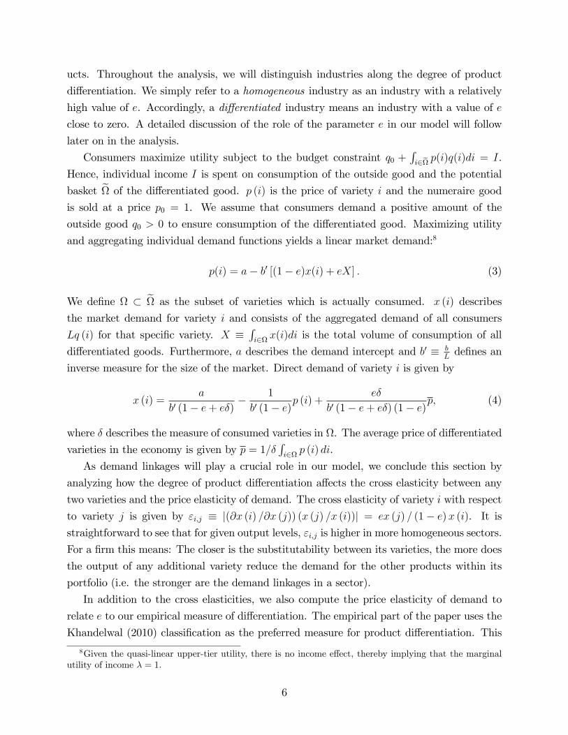
measure is created by evaluating changes in prices conditional on market shares: A product is
classi�ed as more di¤erentiated if the �rm can increase prices without losing market shares.
To connect this to our theoretical model, we compute the price elasticity of demand and
show how it responds to a change in the degree of di¤erentiation in a sector. Given the
linear demand system in Eq. (3), there exists an upper bound of the price, where demand
x(i) is just driven to zero:
pmax � (1� e) a+ e�p(1� e+ e�) . (5)
Following Melitz and Ottaviano (2008), we express the price elasticity of demand as
"i �����@x (i)@p (i)
p (i)
x (i)
���� = p (i)
(pmax � p (i)) , (6)
by combining Eqs. (4) and (5). Inspecting the latter expression clari�es the role of the
degree of product di¤erentiation e in determining the demand linkages in our model. It can
easily be shown that, ceteris paribus, the choke price pmax decreases and, therefore, the price
elasticity "i increases when products become more homogeneous.
@pmax
@ejp;�=const= �
� (a� p)(1� e+ e�)2
< 0. (7)
This implies that the parameter e in our theoretical model is closely related to the Khandelwal
(2010) measure of di¤erentiation which we use in the empirical part of our paper.
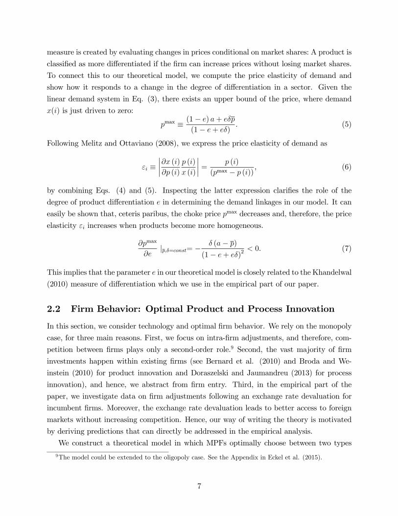
2.2 Firm Behavior: Optimal Product and Process Innovation
In this section, we consider technology and optimal �rm behavior. We rely on the monopoly
case, for three main reasons. First, we focus on intra-�rm adjustments, and therefore, com-
petition between �rms plays only a second-order role.9 Second, the vast majority of �rm
investments happen within existing �rms (see Bernard et al. (2010) and Broda and We-
instein (2010) for product innovation and Doraszelski and Jaumandreu (2013) for process
innovation), and hence, we abstract from �rm entry. Third, in the empirical part of the
paper, we investigate data on �rm adjustments following an exchange rate devaluation for
incumbent �rms. Moreover, the exchange rate devaluation leads to better access to foreign
markets without increasing competition. Hence, our way of writing the theory is motivated
by deriving predictions that can directly be addressed in the empirical analysis.
We construct a theoretical model in which MPFs optimally choose between two types
9The model could be extended to the oligopoly case. See the Appendix in Eckel et al. (2015).
7

of investment. Firstly, �rms invest in new product lines and thereby extend their product
portfolio. Secondly, �rms may decide for each of their products how much to invest in
the production technology. Both types of investment depend on the degree of product
di¤erentiation through the demand and cost linkages taken into account by a �rm. In the
previous section, we have already introduced the demand linkages into our model. We argue
that the demand linkages in particular determine the returns to product innovation. While
deciding on the optimal number of products, the �rm considers the negative impact of the
marginal good on the demand for the rest of its products. Hence, the more similar are the
products within the portfolio, the stronger will be the cannibalization e¤ect of the marginal
variety. Consequently, we show that the optimal product range will be smaller in a more
homogeneous sector.
As a novel feature of our model, we introduce cost linkages and relate them to the degree
of product di¤erentiation. In particular, the strength of the cost-linkages determines the
returns to process innovation in our model. Firms may decide for each product how much
to invest. However, we argue that there are intra-�rm spillover e¤ects between the varieties.
This means that a �rm can use parts of the process R&D of one product for other products
in its portfolio. To which extent product-speci�c R&D is applicable to other processes
depends on the similarity of production processes and, therefore, on the degree of product
di¤erentiation. Thus, �rms in homogeneous sectors will invest more in process innovation as
they can internalize more spillovers between production lines.
Production Technology Production is characterized by �exible manufacturing. We fol-
low Eckel and Neary (2010) and assume that �rms have a core competence i = 0, which
denotes the product where the �rm is most e¢ cient in production. Besides the core variety,
an MPF can produce additional varieties with rising marginal costs. Production costs for
variety i without investments are given by c (i) = c + c1i. For the sake of simplicity, we
assume a linear cost function, though this is not required to derive our results.
Firms can reduce production costs through variety speci�c process innovation. Further-
more, we allow for investment spillovers between products. To reduce production costs of
variety i, a �rm undertakes process innovation k (i) which reduces production costs at a
diminishing rate. The variety speci�c costs savings from innovation are given by 2k (i)0:5.
As mentioned earlier, part of the process optimization of one variety is applicable to all other
varieties, which implies that production of variety i bene�ts from all investments undertaken
on all the other products K�i �Rni k (i)
0:5 di. The degree to which knowledge is applicable
8

to other products depends on the spillover parameter
� (e) 2 (0; 1) with �0 (e) > 0. (8)
� (e) is a key parameter of our model which captures the idea that more homogenous products
also imply more similar production processes. Therefore, product speci�c investments are
better applicable to the entire product portfolio in a more homogenous sector leading to
higher investment spillovers between similar products. We will de�ne a functional form for
this parameter later on in the analysis.
Considering these aspects, production costs of variety i are given by:
c (i) = c+ c1i��2k (i)0:5 + 2� (e)K�i
�: (9)
This can be rearranged to
c (i) = c+ c1i��2 (1� � (e)) k (i)0:5 + 2� (e)K
�, (10)
where in analogy to X, K =R �0k (i)0:5 di denotes total investment in process innovation.
Pro�t Maximization In our setup, an MPF simultaneously chooses optimal scale x (i)
and process innovation k (i) per product as well as optimal product scope �. Process inno-
vation is carried out at a rate rk and product innovation requires building a new production
line at a rate r�. Total pro�ts are given by:
� =
Z �
0
�p(i)� c� c1i+ 2 (1� � (e)) k (i)0:5 + 2� (e)K
�x(i)di�
Z �
0
rkk (i) di� �r�. (11)
Optimal Scale Maximizing pro�ts in Eq. (11) with respect to scale x (i) implies the
following �rst-order condition:10
@�
@x(i)= p(i)� c� c1i+ 2 (1� � (e)) k (i)0:5 + 2� (e)K � b0 (1� e)x (i)� b0eX = 0. (12)
Using the inverse demand in Eq. (3) and solving for x (i) yields optimal scale of variety i:
x(i) =a� c� c1i+ 2 (1� � (e)) k (i)0:5 + 2� (e)K � 2b0eX
2b0(1� e) . (13)
10The second-order condition is negative: @2�@x(i)2
= �2b0 < 0.
9

Furthermore, we derive total �rm scale X by integrating over x (i) in Eq. (13):
X =��a� c� c1 �2
�+ 2 (1� � (e) + � (e) �)K
2b0(1� e+ e�) . (14)
Inspection of Eq. (13) reveals the two opposing linkage e¤ects arising from the degree of
product di¤erentiation in a sector. On the one hand, there is a demand linkage (cannibal-
ization) of total �rm�s scale X on the output of a single variety
@x (i)
@X= � e
1� e < 0, (15)
whereby the negative impact increases in e. On the other hand, with rising values of e the
cost linkages (spillovers) from other varieties become more prominent:
@x (i)
@K=
� (e)
b0 (1� e) > 0. (16)
As a result of the underlying cost structure with �exible manufacturing, optimal scale of
the core product is the largest, and output per variety diminishes with distance to the core
product. We illustrate the output scheme in Figure 1, where �0�� indicates the di¤erence
in scale between the core and marginal product in the portfolio. The exact mathematical
expression for �0�� is determined later on in the analysis.
Figure 1: Output Schedule
( )ix
i
δ−∆0
δ
Substituting optimal scale in Eq. (13) into the inverse demand gives the optimal pricing
10
schedule, with the lowest price charged for the core product:
p(i) =1
2
�a+ c+ c1i� 2 (1� � (e)) k (i)0:5 � 2� (e)K
�. (17)
The latter explains why the output of the core competency is sold at the highest scale.
Finally, the price-cost margin for variety i is given by:
p (i)� c (i) = a� c� c1i+ 2 (1� � (e)) k (i)0:5 + 2� (e)K2
. (18)
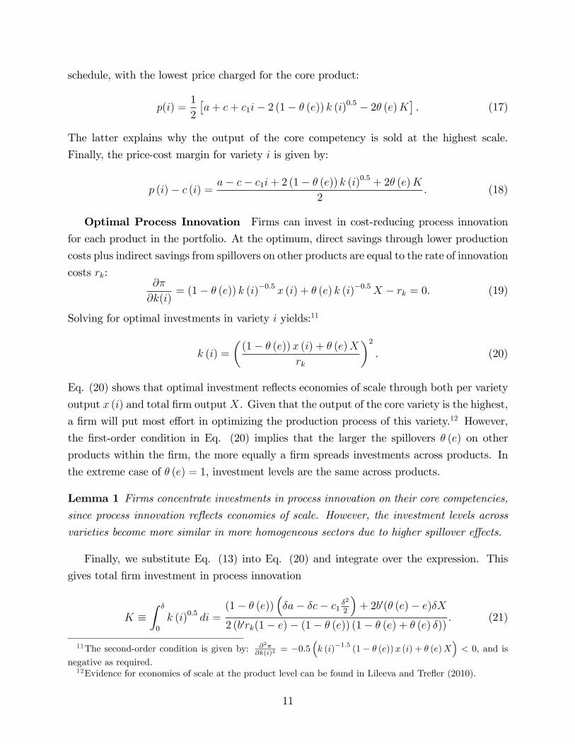
Optimal Process Innovation Firms can invest in cost-reducing process innovation
for each product in the portfolio. At the optimum, direct savings through lower production
costs plus indirect savings from spillovers on other products are equal to the rate of innovation
costs rk:@�
@k(i)= (1� � (e)) k (i)�0:5 x (i) + � (e) k (i)�0:5X � rk = 0. (19)
Solving for optimal investments in variety i yields:11
k (i) =
�(1� � (e))x (i) + � (e)X
rk
�2. (20)
Eq. (20) shows that optimal investment re�ects economies of scale through both per variety
output x (i) and total �rm outputX. Given that the output of the core variety is the highest,
a �rm will put most e¤ort in optimizing the production process of this variety.12 However,
the �rst-order condition in Eq. (20) implies that the larger the spillovers � (e) on other
products within the �rm, the more equally a �rm spreads investments across products. In
the extreme case of � (e) = 1, investment levels are the same across products.
Lemma 1 Firms concentrate investments in process innovation on their core competencies,since process innovation re�ects economies of scale. However, the investment levels across
varieties become more similar in more homogeneous sectors due to higher spillover e¤ects.
Finally, we substitute Eq. (13) into Eq. (20) and integrate over the expression. This
gives total �rm investment in process innovation
K �Z �
0
k (i)0:5 di =(1� � (e))
��a� �c� c1 �
2
2
�+ 2b0(� (e)� e)�X
2 (b0rk(1� e)� (1� � (e)) (1� � (e) + � (e) �)). (21)
11The second-order condition is given by: @2�@k(i)2 = �0:5
�k (i)
�1:5(1� � (e))x (i) + � (e)X
�< 0, and is
negative as required.12Evidence for economies of scale at the product level can be found in Lileeva and Tre�er (2010).
11
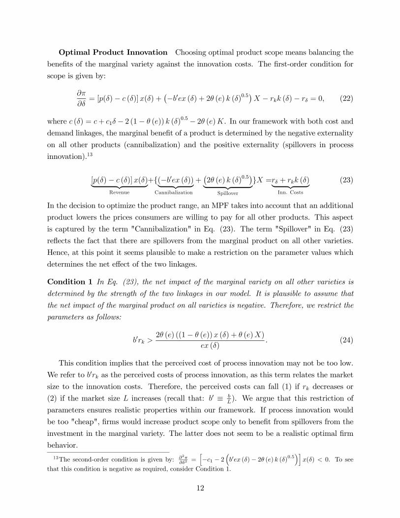
Optimal Product Innovation Choosing optimal product scope means balancing the
bene�ts of the marginal variety against the innovation costs. The �rst-order condition for
scope is given by:
@�
@�= [p(�)� c (�)]x(�) +
��b0ex (�) + 2� (e) k (�)0:5
�X � rkk (�)� r� = 0, (22)
where c (�) = c+ c1�� 2 (1� � (e)) k (�)0:5 � 2� (e)K. In our framework with both cost anddemand linkages, the marginal bene�t of a product is determined by the negative externality
on all other products (cannibalization) and the positive externality (spillovers in process
innovation).13
[p(�)� c (�)]x(�)| {z }Revenue
+f(�b0ex (�))| {z }Cannibalization
+�2� (e) k (�)0:5
�| {z }Spillover
gX =r� + rkk (�)| {z }Inn. Costs
(23)
In the decision to optimize the product range, an MPF takes into account that an additional
product lowers the prices consumers are willing to pay for all other products. This aspect
is captured by the term "Cannibalization" in Eq. (23). The term "Spillover" in Eq. (23)
re�ects the fact that there are spillovers from the marginal product on all other varieties.
Hence, at this point it seems plausible to make a restriction on the parameter values which
determines the net e¤ect of the two linkages.
Condition 1 In Eq. (23), the net impact of the marginal variety on all other varieties isdetermined by the strength of the two linkages in our model. It is plausible to assume that
the net impact of the marginal product on all varieties is negative. Therefore, we restrict the
parameters as follows:
b0rk >2� (e) ((1� � (e))x (�) + � (e)X)
ex (�). (24)
This condition implies that the perceived cost of process innovation may not be too low.
We refer to b0rk as the perceived costs of process innovation, as this term relates the market
size to the innovation costs. Therefore, the perceived costs can fall (1) if rk decreases or
(2) if the market size L increases (recall that: b0 � bL). We argue that this restriction of
parameters ensures realistic properties within our framework. If process innovation would
be too "cheap", �rms would increase product scope only to bene�t from spillovers from the
investment in the marginal variety. The latter does not seem to be a realistic optimal �rm
behavior.
13The second-order condition is given by: @2�@�2
=h�c1 � 2
�b0ex (�)� 2� (e) k (�)0:5
�ix(�) < 0. To see
that this condition is negative as required, consider Condition 1.
12

In the following, we express a �rm�s optimal scope in terms of scale of the marginal
product x (�). To do so, we substitute the output of the marginal variety from Eq. (13) and
its respective price-cost margin from Eq. (18) into the �rst-order condition for scope (22):
x (�) =
srkk (�) + r� � 2� (e) k (�)0:5X
b0 (1� e) . (25)
Considering again Figure 1, the latter expression can be interpreted as follows: The lower is
the output of the marginal variety �, the larger is the product range o¤ered by the �rm.
To provide some further insights into our model, we combine the �rst-order conditions
for scale and scope in Eqs. (13) and (25), to derive an alternative expression for optimal
scale:
x (i) =c1 (� � i) + 2 (1� � (e))
�k (i)0:5 � k (�)0:5
�2b0(1� e) +
srkk (�) + r� � 2� (e) k (�)0:5X
b0 (1� e) . (26)
It is straightforward to see that this expression boils down to Eq. (25) by setting i = � for
the marginal variety. Furthermore, we can use this expression to calculate the di¤erence in
scale of the core (i = 0) versus the marginal variety �, illustrated in Figure 1:
�0�� =c1�
2�b0(1� e)� (1��(e))2
rk
� . (27)
Since the underlying technology is �exible manufacturing, the di¤erence in output increases
in the product range �. The larger is the distance to the core product, the lower will be
the e¢ ciency of the marginal product. The latter e¤ect is magni�ed for higher values of
c1, as this variable determines how much marginal costs increase with rising distance to the
core product. Moreover, �0�� decreases in the strength of the spillovers � (e). As stated in
Lemma 1, �rms concentrate their investment in process R&D on the core varieties. However,
if spillover e¤ects are large, the marginal varieties bene�t more from the investments in the
high-scale core varieties.
Lemma 2 The di¤erence in scale between the core and the marginal variety is determinedby the di¤erence in production costs of the two varieties. The productivity of the marginal
product falls with distance to the core product and rises in the degree of spillovers.
13
2.3 Comparative Statics
In the previous section, we established the baseline theoretical framework. In the next step,
we derive the main predictions that we test in the empirical section. To start with, we analyze
the e¤ects of an increase in the market size L (lower values of b0) on optimal investment levels.
Furthermore, we investigate optimal investment strategies in sectors with di¤erent degrees
of product di¤erentiation. To derive our results, we follow the solution path in Eckel and
Neary (2010), and express the equilibrium equations in terms of X and � only. Moreover, as
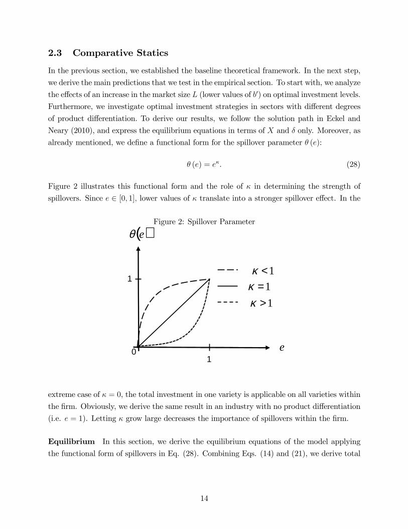
already mentioned, we de�ne a functional form for the spillover parameter � (e):
� (e) = e�. (28)
Figure 2 illustrates this functional form and the role of � in determining the strength of
spillovers. Since e 2 [0; 1]; lower values of � translate into a stronger spillover e¤ect. In the
Figure 2: Spillover Parameter
( )eθ
1
0 e1
1=κ1>κ
1<κ
extreme case of � = 0, the total investment in one variety is applicable on all varieties within
the �rm. Obviously, we derive the same result in an industry with no product di¤erentiation
(i.e. e = 1). Letting � grow large decreases the importance of spillovers within the �rm.
Equilibrium In this section, we derive the equilibrium equations of the model applying
the functional form of spillovers in Eq. (28). Combining Eqs. (14) and (21), we derive total
14

�rm scale as:
X =��a� c� c1 �2
�2�b0(1� e+ e�)� (1�e�+e��)2
rk
� . (29)
The term (1�e�+e��)2rk
re�ects cost-savings from process innovation, which induces a �rm to
increase total �rm scale X. Clearly, the strength of the latter e¤ect is mitigated by the
costs for process innovation rk. Plugging Eq. (29) back into Eq. (21) yields total process
innovation as:
K =(1� e� + e��)
rkX. (30)
The parameter � determines the strength of spillovers, where total process innovation is the
largest for � = 0. Inspecting Eqs. (29) and (30) in detail reveals that investments in process
innovation decrease with rising levels of �, i.e. @K@�< 0. Furthermore, process innovation K
re�ects economies of scale as it depends on total �rm scale X. Using information from Eqs.
(20), (29), and (30) together with Eq. (13), we can express optimal scale per variety as:
x (i) =a� c� c1i� 2
�b0e� e�(2(1�e�)+e��)
rk
�X
2�b0(1� e)� (1�e�)2
rk
� . (31)
Within our framework, we have two opposing e¤ects of total scale X on per variety output.
On the one hand, rising total output induces the �rm to invest more in process innovation,
which increases per variety output. On the other hand, rising total scale intensi�es cannibal-
ization within the portfolio. The latter e¤ect reduces per variety output. However, Condition
1 stated in Eq. (24) guarantees that the spillover e¤ect cannot dominate the cannibalization
e¤ect, i.e. @x(i)@X
< 0.
Finally, substituting from Eq. (20) into Eq. (25), we express the �rst-order condition for
scope as:
x (�) =
vuuut r� � (e�X)2
rk�b0 (1� e)� (1�e�)2
rk
� . (32)
The formal derivation of this expression is presented in the Appendix. Eq. (32) implicitly
de�nes product scope � in terms of the output of the marginal variety. Solving for � gives
the explicit expression for product scope:
� =
a� c� 2r�
b0 (1� e)� (1�e�)2rk
��r� � e2�X2
rk
�� 2
�b0e� 2e�(1�e�)
rk
�X�
c1 � 2e2�Xrk
� . (33)
15
Eqs. (32) and (33) reveal that higher costs for product innovation r� decrease the optimal
product range. The latter implies a higher output of the marginal variety � (see Eq. (32)).
Referring to Figure 1, this characterizes a variety closer to the �rm�s core competence.
Inspecting the term 2p� in Eq. (33) reveals the multiplicative structure of the inverse
measure for market size (b0 � bL) and the cost for product innovation r�. This structure
translates an increase in the market size L into lower perceived costs of product innovation
for the �rm.
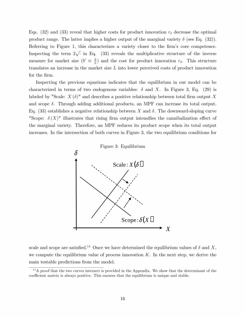
Inspecting the previous equations indicates that the equilibrium in our model can be
characterized in terms of two endogenous variables: � and X. In Figure 3, Eq. (29) is
labeled by "Scale: X (�)" and describes a positive relationship between total �rm output X
and scope �. Through adding additional products, an MPF can increase its total output.
Eq. (33) establishes a negative relationship between X and �. The downward-sloping curve
"Scope: � (X)" illustrates that rising �rm output intensi�es the cannibalization e¤ect of
the marginal variety. Therefore, an MPF reduces its product scope when its total output
increases. In the intersection of both curves in Figure 3, the two equilibrium conditions for
Figure 3: Equilibrium
δ
X( )Xδ:Scope
( )δX:Scale
scale and scope are satis�ed.14 Once we have determined the equilibrium values of � and X,
we compute the equilibrium value of process innovation K. In the next step, we derive the
main testable predictions from the model.
14A proof that the two curves intersect is provided in the Appendix. We show that the determinant of thecoe¢ cient matrix is always positive. This ensures that the equilibrium is unique and stable.
16
The E¤ects of a Larger Market Size We are interested in the e¤ects of globalization
on product and process innovation. We follow Krugman (1979) and interpret globalization
as an increase in the number of consumers L. As we analyze the behavior of a single MPF,
we neglect the competition e¤ect of globalization. This modeling choice is motivated by
the nature of our empirical analysis, where we investigate the e¤ect of a devaluation of
the Brazilian real. For Brazilian exporters, a devaluation means improved access to foreign
markets since products become cheaper. Therefore, Brazilian �rms can gain foreign market
shares without losing domestic market shares.
An increase in the market size L reduces the slope b0 of the demand function in Eq. (3).
In the Appendix, we derive the total derivatives of the equilibrium conditions in terms of
scale X (Eq. (29)) and scope � (Eq. (33)), which lead to the following results.
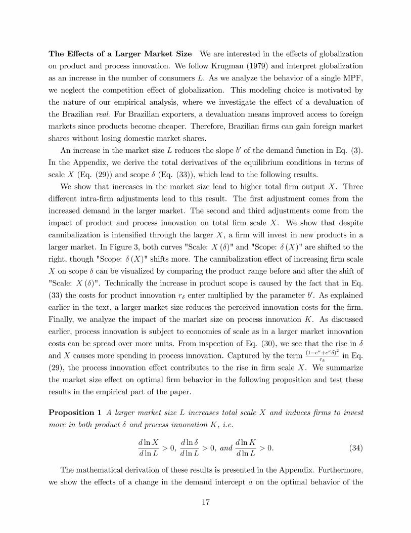
We show that increases in the market size lead to higher total �rm output X. Three
di¤erent intra-�rm adjustments lead to this result. The �rst adjustment comes from the
increased demand in the larger market. The second and third adjustments come from the
impact of product and process innovation on total �rm scale X. We show that despite
cannibalization is intensi�ed through the larger X, a �rm will invest in new products in a
larger market. In Figure 3, both curves "Scale: X (�)" and "Scope: � (X)" are shifted to the
right, though "Scope: � (X)" shifts more. The cannibalization e¤ect of increasing �rm scale
X on scope � can be visualized by comparing the product range before and after the shift of
"Scale: X (�)". Technically the increase in product scope is caused by the fact that in Eq.
(33) the costs for product innovation r� enter multiplied by the parameter b0. As explained
earlier in the text, a larger market size reduces the perceived innovation costs for the �rm.
Finally, we analyze the impact of the market size on process innovation K. As discussed
earlier, process innovation is subject to economies of scale as in a larger market innovation
costs can be spread over more units. From inspection of Eq. (30), we see that the rise in �
and X causes more spending in process innovation. Captured by the term (1�e�+e��)2rk
in Eq.
(29), the process innovation e¤ect contributes to the rise in �rm scale X. We summarize
the market size e¤ect on optimal �rm behavior in the following proposition and test these
results in the empirical part of the paper.
Proposition 1 A larger market size L increases total scale X and induces �rms to invest
more in both product � and process innovation K, i.e.
d lnX
d lnL> 0,
d ln �
d lnL> 0, and
d lnK
d lnL> 0. (34)
The mathematical derivation of these results is presented in the Appendix. Furthermore,
we show the e¤ects of a change in the demand intercept a on the optimal behavior of the
17

�rm. The latter comparative static yields qualitatively the same results.
Sectors with Di¤erent Scope for Product Di¤erentiation We derive a second testable
prediction of our model with respect to the degree of product di¤erentiation in a sector. A
simple comparison between brick production and the automotive sector makes it clear that
there is a lot more scope for di¤erentiation in the latter sector. We argue that the degree of
di¤erentiation is crucial in explaining the innovation behavior of �rms. Recall, that degree
of di¤erentiation determines the strength of the two linkages within our framework. A low
degree of di¤erentiation (high e) causes high cannibalization and high spillover e¤ects and,
therefore, promotes process innovation. One can think again of our example of an MPF pro-
ducing bricks that are slightly di¤erentiated. It is plausible to assume that a large fraction of
the investment in the production line of one speci�c brick is applicable to the production of
all other bricks produced by the same �rm. However, introducing one further brick will have
a strong cannibalizing impact on the initial portfolio. Di¤erentiating Eq. (30) with respect
to the degree of product di¤erentiation e keeping �rm size �xed con�rms our intuition:
@ lnK
@ ln e=
�e� (� � 1)(1� e� + e��) > 0. (35)
Let us now assume the other extreme case of a highly di¤erentiated industry, in our
example the automotive sector. Assuming that cars are more di¤erentiated than bricks,
optimizing the production process for one speci�c car will have positive but lower spillovers
on the other cars in comparison to the case of (more homogeneous) bricks. The more
di¤erentiated two cars are, the lower will be the number of identical parts used in production
and, therefore, the lower will be the spillovers in production. However, for a �rm producing
multiple cars, the negative externality of adding an additional car declines the higher is the
degree of di¤erentiation (i.e. the lower is the cannibalization e¤ect). Again, we hold �rm
size �xed and di¤erentiate Eq. (33) with respect to the degree of product di¤erentiation
e. There are two opposing channels at work when considering the e¤ect of the degree of
product di¤erentiation on the product range �. On the one hand, the marginal product
cannibalizes, on the other hand, all initial products bene�t from process-spillovers from
the marginal product. Di¤erentiating Eq. (33) with respect to e leads to a cumbersome
expression, which is presented in the Appendix. Here we show the solution for the case of
the strongest spillover e¤ects. The following derivative reveals that even in this case the
cannibalization e¤ect dominates, which con�rms our intuition.
lim�!0
@ ln �
@ ln e= �b
0e (2X � x (�))�c1 � 2X
rk
��
< 0 (36)
18
The derivation of this expression and further discussion are presented in the Appendix.
We summarize the e¤ect of the degree of product di¤erentiation on optimal innovation
behavior in the following proposition and test the results in the empirical part of the paper.
Proposition 2 Conditional on �rm size, �rms in sectors with a large (low) scope for prod-
uct di¤erentiation will invest more in product (process) innovation. This behavior is caused
by the lower (stronger) demand- and lower (stronger) cost-linkages in a di¤erentiated (ho-
mogeneous) sector.
3 Data
We test the main predictions of the model using Brazilian �rm-level data. For the main
results, we use data for the period 1998-2000. In robustness checks and a falsi�cation exercise,
we extend the analysis for the years 2000-2005. Firm-level data are matched using the unique
�rm tax number and come from two main sources: (i) SECEX (Foreign Trade Secretariat),
which provides information on the universe of products exported by Brazilian �rms and
(ii) Innovation survey from PINTEC (Brazilian Firm Industrial Innovation Survey). We
combine �rm-level data with industry-level data to investigate how di¤erent industries react
to a trade shock in terms of their investments in innovation.
A distinctive feature of the data is the availability of highly detailed information on �rm-
level innovation investments, including several dimensions of product and process innovation.
A further distinctive feature of the data is the event of a major and largely unexpected ex-
change rate shock in the period under analysis. The devaluation made Brazilian products
more competitive in both domestic and foreign markets and, therefore, increased incentives
for �rms to innovate (due to scale e¤ects). However, �rms react in di¤erent ways to the trade
shock depending on the degree of product di¤erentiation of the industry: While more ho-
mogeneous industries have higher incentives to invest more in process innovation because of
spillover e¤ects, di¤erentiated industries have higher incentives to invest in product innova-
tion because of lower cannibalization across products. To tackle this issue, we use information
on di¤erent types of innovation combined with the degree of product di¤erentiation of the
industry.
19
3.1 Innovation Variables
The innovation survey provides detailed information on innovation investments of 3,070
manufacturing exporters for which we can exploit time-varying information.15 The main
questions used in our study for product and process innovation are: 1. Did the �rm introduce
a new product in the period? (product innovation) and 2. Did the �rm introduce new
production processes in the period? (process innovation). Using this information, we create
the variables Productf = 1 if a �rm f in industry i reported important e¤orts to do product
innovation (zero otherwise), and Processf = 1 if the �rm reported process innovation (zero
otherwise).
Product innovation does not necessarily mean an increase in product scope (suggested by
our theory), since �rms could simultaneously add and drop varieties or change the attributes
of existent varieties. Therefore, in order to get closer to our theoretical mechanism, we use a
further question from the survey related to product scope: 3. Importance of the innovation to
increase product scope, Scopef . This categorical variable (with four degrees of importance)
relates innovation to increases in product scope. We transform this variable in a dummy
Scopef = 1 if the �rm reports that it was important or very important to increase scope
(and zero otherwise).
For process innovation, the variable Processf may also not be directly related to the
mechanism we propose in the theory (that some �rms internalize spillover e¤ects and, there-
fore, invest more in process innovation). Thus, to evaluate the importance of spillover e¤ects,
we use information related to increases in the �exibility of the production process. In par-
ticular, we use the following question from the survey: 4. Importance of the innovation to
increase production �exibility, Flexibilityf . Flexibilityf is a categorical variable (with four
degrees of importance) related to the ability of the �rm to make the production process more
�exible and increase the spillover e¤ects among production lines. Therefore, it is consistent
with the mechanism of the theoretical model, predicting that �rms may internalize intra-�rm
spillover e¤ects. The description of variables is found in Table 14 in the Appendix.
The data has the disadvantage of not capturing di¤erences in the intensity of innovation
across �rms (variables are at most categorical, but not continuous). However, for the pur-
poses of our study, we are able to capture the relevant mechanism, referring to the variation
in innovation e¤orts across industries.
Table 1 presents summary statistics for the baseline indicators of innovation in 2000,
following the exchange rate shock.16 About half of the �rms reported changes in process and
15The PINTEC (2000) survey provides information for a total of 3,700 �rms. However, for 630 of theminformation for many variables of interest is only available for the year 2000.16Values are based on a sample of 3,070 �rms (sample used in the paper).
20
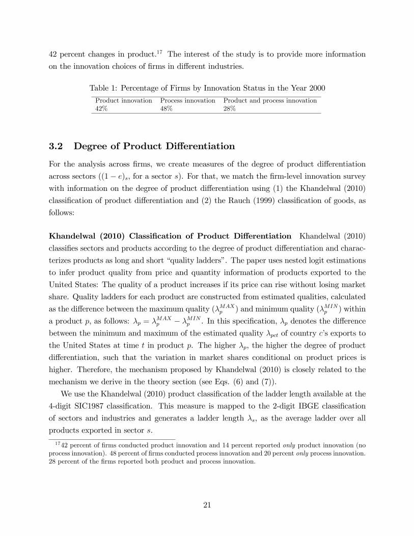
42 percent changes in product.17 The interest of the study is to provide more information
on the innovation choices of �rms in di¤erent industries.
Table 1: Percentage of Firms by Innovation Status in the Year 2000
Product innovation Process innovation Product and process innovation42% 48% 28%
3.2 Degree of Product Di¤erentiation
For the analysis across �rms, we create measures of the degree of product di¤erentiation
across sectors ((1� e)s, for a sector s). For that, we match the �rm-level innovation surveywith information on the degree of product di¤erentiation using (1) the Khandelwal (2010)
classi�cation of product di¤erentiation and (2) the Rauch (1999) classi�cation of goods, as
follows:
Khandelwal (2010) Classi�cation of Product Di¤erentiation Khandelwal (2010)
classi�es sectors and products according to the degree of product di¤erentiation and charac-
terizes products as long and short �quality ladders�. The paper uses nested logit estimations
to infer product quality from price and quantity information of products exported to the
United States: The quality of a product increases if its price can rise without losing market
share. Quality ladders for each product are constructed from estimated qualities, calculated
as the di¤erence between the maximum quality (�MAXp ) and minimum quality (�MIN
p ) within
a product p, as follows: �p = �MAXp � �MIN
p . In this speci�cation, �p denotes the di¤erence
between the minimum and maximum of the estimated quality �pct of country c�s exports to
the United States at time t in product p. The higher �p, the higher the degree of product
di¤erentiation, such that the variation in market shares conditional on product prices is
higher. Therefore, the mechanism proposed by Khandelwal (2010) is closely related to the
mechanism we derive in the theory section (see Eqs. (6) and (7)).
We use the Khandelwal (2010) product classi�cation of the ladder length available at the
4-digit SIC1987 classi�cation. This measure is mapped to the 2-digit IBGE classi�cation
of sectors and industries and generates a ladder length �s, as the average ladder over all
products exported in sector s.
1742 percent of �rms conducted product innovation and 14 percent reported only product innovation (noprocess innovation). 48 percent of �rms conducted process innovation and 20 percent only process innovation.28 percent of the �rms reported both product and process innovation.
21
Rauch (1999) Classi�cation of Goods Rauch (1999) classi�es trade data into three
groups of commodities:w, homogeneous (organized exchange) goods, which are goods tradedin an organized exchange; r, reference priced goods, not traded in an organized exchange, butwhich have some quoted reference price, such as industry publications; and n, di¤erentiatedgoods, without any quoted price. Using this classi�cation at the 4-digit SITC product
classi�cation (issued by the United Nations), we create a measure of the share of products
from a �rm classi�ed as di¤erentiated goods: ShDiffs =Nproductss;n
Nproductss;(w+r+n), where ShDiffs
is the share of products produced by sector s classi�ed as di¤erentiated goods. Also in this
case, we map the Rauch (1999) classi�cation of goods to the 2-digit industry classi�cation
of di¤erentiation from IBGE. Moreover, as an alternative measure, we estimate ShSaless =Salesn
TotalSales(w+r+n), where ShSaless is the share of sales of di¤erentiated products in comparison
to total sales in a sector s.18
We use �s as our benchmark measure, since �s provides higher variation in comparison
to ShDiffs: While �s is created from a continuous variable (product ladder), the Rauch
(1999) classi�cation is created from a binary variable (products classi�ed as di¤erentiated or
non-di¤erentiated goods). Thus, ShDiffs may be inaccurate and subject to measurement
error. We keep the Rauch (1999) classi�cation for robustness checks. Summary statistics for
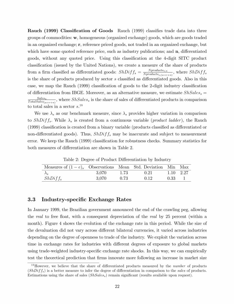
both measures of di¤erentiation are shown in Table 2.
Table 2: Degree of Product Di¤erentiation by Industry
Measures of (1� e)s Observations Mean Std. Deviation Min Max�s 3,070 1.73 0.21 1.10 2.27ShDiffs 3,070 0.73 0.12 0.33 1
3.3 Industry-speci�c Exchange Rates
In January 1999, the Brazilian government announced the end of the crawling peg, allowing
the real to free �oat, with a consequent depreciation of the real by 25 percent (within a
month). Figure 4 shows the evolution of the exchange rate in this period. While the size of
the devaluation did not vary across di¤erent bilateral currencies, it varied across industries
depending on the degree of openness to trade of the industry. We exploit the variation across
time in exchange rates for industries with di¤erent degrees of exposure to global markets
using trade-weighted industry-speci�c exchange rate shocks. In this way, we can empirically
test the theoretical prediction that �rms innovate more following an increase in market size
18However, we believe that the share of di¤erentiated products measured by the number of products(ShDiffs) is a better measure to infer the degree of di¤erentiation in comparison to the sales of products.Estimations using the share of sales (ShSaless) remain signi�cant (results available upon request).
22
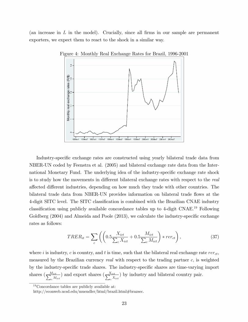
(an increase in L in the model). Crucially, since all �rms in our sample are permanent
exporters, we expect them to react to the shock in a similar way.
Figure 4: Monthly Real Exchange Rates for Brazil, 1996-2001
Industry-speci�c exchange rates are constructed using yearly bilateral trade data from
NBER-UN coded by Feenstra et al. (2005) and bilateral exchange rate data from the Inter-
national Monetary Fund. The underlying idea of the industry-speci�c exchange rate shock
is to study how the movements in di¤erent bilateral exchange rates with respect to the real
a¤ected di¤erent industries, depending on how much they trade with other countries. The
bilateral trade data from NBER-UN provides information on bilateral trade �ows at the
4-digit SITC level. The SITC classi�cation is combined with the Brazilian CNAE industry
classi�cation using publicly available concordance tables up to 4-digit CNAE.19 Following
Goldberg (2004) and Almeida and Poole (2013), we calculate the industry-speci�c exchange
rates as follows:
TRERit =Xc
��0:5
XictPcXict
+ 0:5MictPcMict
�� rerct
�, (37)
where i is industry, c is country, and t is time, such that the bilateral real exchange rate rerct,
measured by the Brazilian currency real with respect to the trading partner c, is weighted
by the industry-speci�c trade shares. The industry-speci�c shares are time-varying import
shares ( MictPcMict
) and export shares ( XictPcXict) by industry and bilateral country pair.
19Concordance tables are publicly available at:http://econweb.ucsd.edu/muendler/html/brazil.html#brazsec.
23
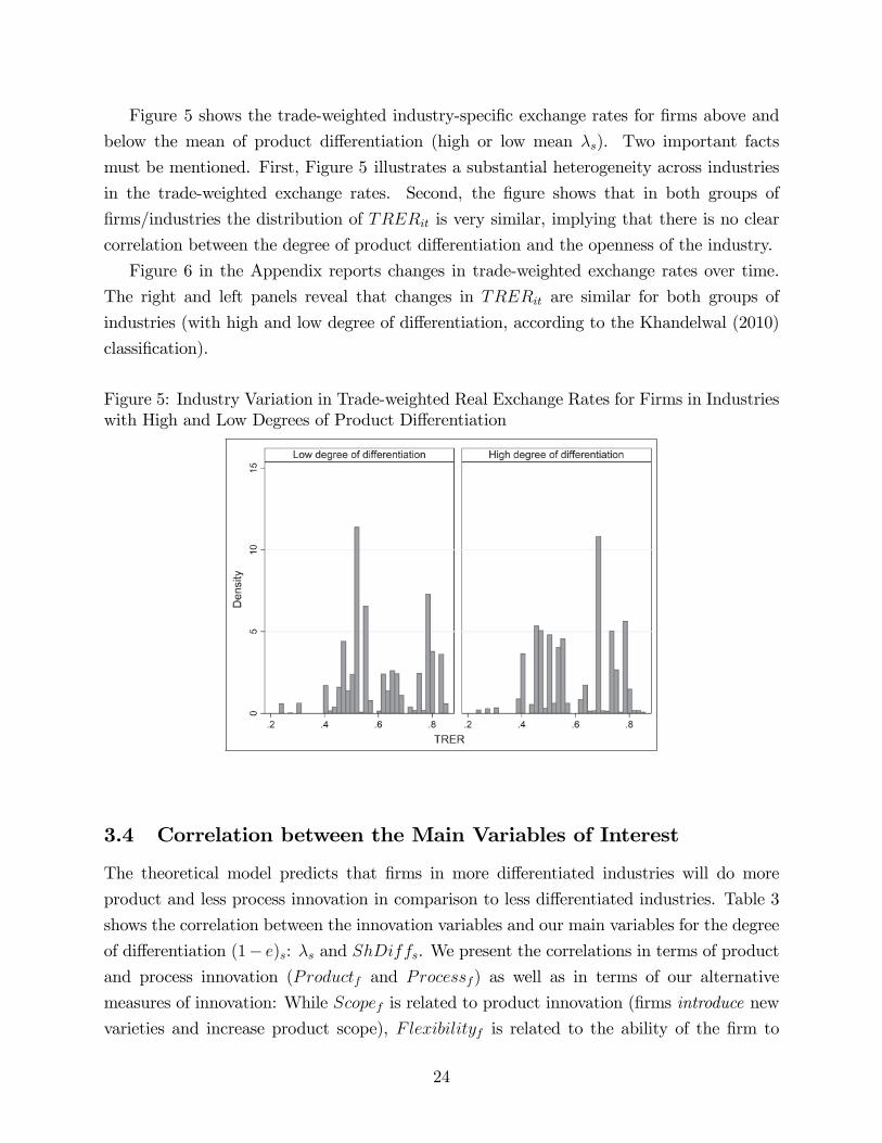
Figure 5 shows the trade-weighted industry-speci�c exchange rates for �rms above and
below the mean of product di¤erentiation (high or low mean �s). Two important facts
must be mentioned. First, Figure 5 illustrates a substantial heterogeneity across industries
in the trade-weighted exchange rates. Second, the �gure shows that in both groups of
�rms/industries the distribution of TRERit is very similar, implying that there is no clear
correlation between the degree of product di¤erentiation and the openness of the industry.
Figure 6 in the Appendix reports changes in trade-weighted exchange rates over time.
The right and left panels reveal that changes in TRERit are similar for both groups of
industries (with high and low degree of di¤erentiation, according to the Khandelwal (2010)
classi�cation).
Figure 5: Industry Variation in Trade-weighted Real Exchange Rates for Firms in Industrieswith High and Low Degrees of Product Di¤erentiation
3.4 Correlation between the Main Variables of Interest
The theoretical model predicts that �rms in more di¤erentiated industries will do more
product and less process innovation in comparison to less di¤erentiated industries. Table 3
shows the correlation between the innovation variables and our main variables for the degree
of di¤erentiation (1� e)s: �s and ShDiffs. We present the correlations in terms of productand process innovation (Productf and Processf ) as well as in terms of our alternative
measures of innovation: While Scopef is related to product innovation (�rms introduce new
varieties and increase product scope), Flexibilityf is related to the ability of the �rm to
24

increase the spillover e¤ects among production lines.
Table 3: Correlation between the Degree of Di¤erentiation and the Outcome Variables
(1� e)s Productf Processf Scopef Flexibilityf�s 0.249*** -0.108** 0.054*** -0.085***ShDiffs 0.048*** -0.029** 0.016** -0.031*Note: *** indicates 1% signi�cance, ** 5% signi�cance, and * 10% signi�cance.
We show that variables related to product innovation (Productf and Scopef) are pos-
itively correlated with the degree of product di¤erentiation. On the other hand, variables
related to process innovation (Processf and Flexibilityf) are negatively correlated with the
degree of product di¤erentiation. Therefore, results in Table 3 are consistent with the pre-
dictions from the theoretical model. Moreover, in the section on robustness checks, we show
that these correlations are not speci�c to the data we use. We combine innovation data for
Brazilian �rms from the World Bank with industry-level data. The correlations between �sand innovation (Productf and Processf) con�rm our results.
4 Empirical Strategy
Our goal in the empirical part of the paper is to test the predictions from the model regard-
ing investment e¤orts of �rms in industries with di¤erent scope for product di¤erentiation,
following a trade shock. We estimate the incidence of changes in innovation investments
�If as a function of the degree of di¤erentiation (1� e)s in the sector s in which the �rmoperates. To investigate the degree of di¤erentiation (1� e)s, we use two di¤erent measures:�s according to Khandelwal (2010) and ShDiffs following Rauch (1999), as described in the
data section. We are interested in the di¤erential e¤ects for industries with di¤erent degrees
of trade openness, measured by changes in time-varying trade-weighted shocks, �TRERi;
using 2-year di¤erences. In the main results, we use the period 1998-2000 (exchange rates
before and after the devaluation in January 1999), and later on we use information for the
period 2000-2005. The empirical speci�cation follows:
Pr(�If = 1) = F (�1�TRERi + �2�TRERi � (1� e)s + �1�Xf + �s + "f ); (38)
where f indexes the �rm, i indexes the industry, s indexes the sector, and �Xf is a vector of
�rm-level time-varying control variables, as described in Table 14 in the Appendix. Initially,
we include only changes in �rm size, then subsequently we add further control variables.
For simplicity, we omit time subscripts for �, which refer to a 2-year lag. "f is an error
25

term. �s are sector �xed e¤ects, such that we can interpret results within industries in a
given sector.20 �If refers to innovation changes conducted by the �rm over the period,
with �If = �Processf or �Productf . In alternative speci�cations, �If = �Scopef or
�Flexibilityf .
In the theoretical model, we state that when market size grows (L increases), the increase
in market size generates incentives for �rms to innovate because of scale e¤ects. Empirically,
we test changes in market size using a major and unexpected exchange rate shock from
1999 as a source of variation (�rms face varying degrees of exposure to foreign markets,
and hence, in the access to foreign markets). We exploit this event using industry-speci�c
exchange rate shocks computed over time, �TRERi. Following the predictions from the
theoretical model, we expect �1 > 0: An exchange rate devaluation increases incentives for
�rms to innovate (because of better access to foreign markets), in particular in industries
more open to international trade.
On top of that, detailed information on the degree of di¤erentiation ((1�e) in the model)and on the type of innovation allows us to evaluate di¤erential e¤ects across industries
and sectors. The di¤erential e¤ects are shown by �2, our main coe¢ cient of interest. �2captures the di¤erential impact of the trade shock on �rms in di¤erentiated sectors relative
to more homogeneous sectors. In response to the shock, scale e¤ects create natural incentives
for �rms to expand innovation investments. In more di¤erentiated sectors, cannibalization
is lower such that �rms invest more in product innovation, while in homogeneous sectors
spillover e¤ects from innovation are higher such that �rms invest more in process innovation.
Therefore, �2 > 0 in case the dependent variable is �Productf , i.e. �rms in sectors with
a high degree of product di¤erentiation invest more in product innovation, and �2 < 0
when the dependent variable is �Processf (�rms in more di¤erentiated sectors invest less
in process innovation in comparison to �rms in more homogeneous sectors).
Concerning the functional form of equation (37), we estimate our empirical model using
probit and linear probability models.21 We also conduct robustness checks using seemingly
unrelated regressions - SUR, to allow the error terms across equations to be correlated
20Note that in the theory we have used the words sector and industry interchangeably. In the empirics itis important that TRERi and (1 � e)s have di¤erent levels of aggregation, such that the interaction termprovides the relevant variation. Therefore, the fact that both variables come from di¤erent classi�cation ofgoods/industries and are aggregated at di¤erent levels is an advantage of our approach. Moreover, there isno clear correlation between (1� e)s and TRERi or between (1� e)s and �TRERi, as we show in Figures5 and 6. If the correlation was high, the interaction term could capture non linearities between innovationand the independent variables. Using the continuous measure of di¤erentiation, �s , we �nd no statisticallysigni�cant correlation between �s and �TRERi:21The linear probability model has the advantage of being easy to estimate and to interpret the coe¢ cients.
However, though unbiased, it poses important disadvantages. To deal with the concerns with the linearestimation, we estimate a probit model.
26

(equations with �Processf or �Productf as dependent variable).
5 Results
Tables 4 and 5 present the main empirical results from our paper. In Table 4, we �rst
investigate whether changes in market size lead to more innovation. As predicted by the
theoretical model, when the market size grows (L increases) incentives to innovate increase
for all �rms and all types of innovation (�1 > 0). Columns (1) to (4) in Table 4 con�rm that
�1 > 0 for product and process innovation, meaning an increase in the predicted probability
of innovation: Following an industry-speci�c exchange rate devaluation (�TRERi > 0), �rms
have higher incentives to invest in product and process innovation. Results are statistically
signi�cant using LPM and Probit, shown in the odds and even columns, respectively. Unless
otherwise stated, results reported for Probit in the tables include the marginal e¤ects, their
standard errors, and the value of the likelihood function. Marginal e¤ects are computed at
means of all variables (means are reported in Tables 2 and 13). At mean values, the average
marginal e¤ect is around 0.273 for product and 0.305 for process innovation, with a p-value
of 0.001 in both cases, meaning that the e¤ect is signi�cant.
Table 4: E¤ect of �TRERi on Innovation
Dependent variable: �Processf �ProductfProbit LPM Probit LPM(1) (2) (3) (4)
�TRERi 0.305*** 0.296*** 0.273*** 0.259***(0.0872) (0.0819) (0.0846) (0.0778)
Constant yes yes yes yes�logNworkersf yes yes yes yesSector s �xed e¤ects yes yes yes yesLog-pseudolikelihood -1895.239 -1776.380Pseudo R-squared 0.010 0.039R-squared 0.104 0.146Observations 3,070 3,070 3,070 3,070
However, the main interest of the paper refers to the di¤erential e¤ects across sectors and
industries. The di¤erential e¤ects using our main measure of di¤erentiation �s are shown
in Table 5. Results con�rm the main predictions from our theoretical model. Following
an exchange rate devaluation (�TRERi > 0), �rms in industries with a high degree of
product di¤erentiation invest more in product innovation relative to other �rms (�2 > 0 when
�If = �Productf), while �rms in industries with a low degree of product di¤erentiation
invest more in process innovation relative to other �rms (�2 < 0 when �If = �Processf).
27
Results hold for both estimation strategies (Probit and LPM).
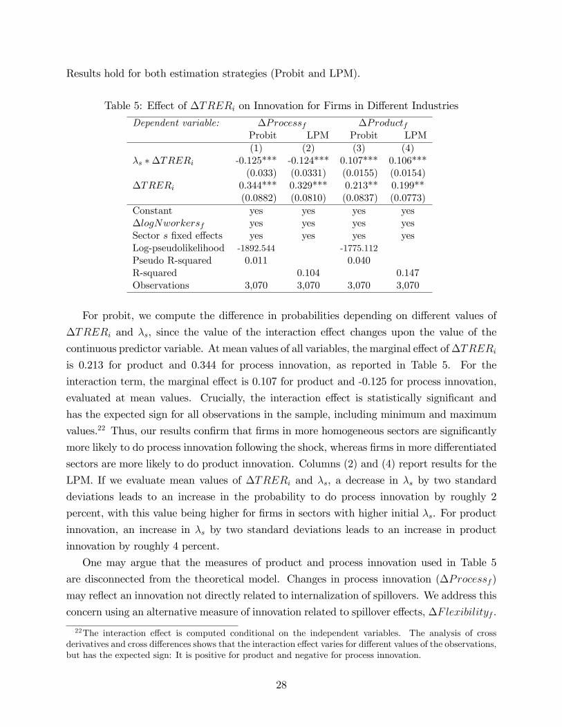
Table 5: E¤ect of �TRERi on Innovation for Firms in Di¤erent Industries
Dependent variable: �Processf �ProductfProbit LPM Probit LPM(1) (2) (3) (4)
�s ��TRERi -0.125*** -0.124*** 0.107*** 0.106***(0.033) (0.0331) (0.0155) (0.0154)
�TRERi 0.344*** 0.329*** 0.213** 0.199**(0.0882) (0.0810) (0.0837) (0.0773)
Constant yes yes yes yes�logNworkersf yes yes yes yesSector s �xed e¤ects yes yes yes yesLog-pseudolikelihood -1892.544 -1775.112Pseudo R-squared 0.011 0.040R-squared 0.104 0.147Observations 3,070 3,070 3,070 3,070
For probit, we compute the di¤erence in probabilities depending on di¤erent values of
�TRERi and �s, since the value of the interaction e¤ect changes upon the value of the
continuous predictor variable. At mean values of all variables, the marginal e¤ect of�TRERiis 0.213 for product and 0.344 for process innovation, as reported in Table 5. For the
interaction term, the marginal e¤ect is 0.107 for product and -0.125 for process innovation,
evaluated at mean values. Crucially, the interaction e¤ect is statistically signi�cant and
has the expected sign for all observations in the sample, including minimum and maximum
values.22 Thus, our results con�rm that �rms in more homogeneous sectors are signi�cantly
more likely to do process innovation following the shock, whereas �rms in more di¤erentiated
sectors are more likely to do product innovation. Columns (2) and (4) report results for the
LPM. If we evaluate mean values of �TRERi and �s, a decrease in �s by two standard
deviations leads to an increase in the probability to do process innovation by roughly 2
percent, with this value being higher for �rms in sectors with higher initial �s. For product
innovation, an increase in �s by two standard deviations leads to an increase in product
innovation by roughly 4 percent.
One may argue that the measures of product and process innovation used in Table 5
are disconnected from the theoretical model. Changes in process innovation (�Processf)
may re�ect an innovation not directly related to internalization of spillovers. We address this
concern using an alternative measure of innovation related to spillover e¤ects, �Flexibilityf .
22The interaction e¤ect is computed conditional on the independent variables. The analysis of crossderivatives and cross di¤erences shows that the interaction e¤ect varies for di¤erent values of the observations,but has the expected sign: It is positive for product and negative for process innovation.
28

Results presented in Table 6 reveal that estimations are robust to this alternative measure
of process innovation.
A similar concern refers to the mechanism related to product innovation (�Productf).
Investments in product innovation may re�ect changes in an already existent product rather
than the creation of an additional variety. We address this concern using an alternative
measure of innovation related to changes in product scope, �Scopef . Results shown in
Table 6 are consistent with the baseline estimations from Table 5.
Table 6: E¤ect of �TRERi on Product Scope and Production Flexibility
Dependent variable: �Scopef �FlexibilityfProbit LPM Probit LPM(1) (2) (3) (4)
�s ��TRERi 0.060*** 0.0497*** -0.0615*** -0.0614***(0.0199) (0.0123) (0.0195) (0.0196)
�TRERi 0.381*** 0.303*** 0.279** 0.272**(0.0889) (0.0548) (0.1171) (0.114)
Constant yes yes yes yes�logNworkersf yes yes yes yesSector s �xed e¤ects yes yes yes yesLog-pseudolikelihood -567.767 -1255.563Pseudo R-squared 0.050 0.019R-squared 0.094 0.069Observations 3,070 3,070 1,971 1,971
6 Robustness Checks
Rauch (1999) Measure of Product Di¤erentiation We use ShDiffs as an alternative
measure to �s and replicate the interaction e¤ects from Table 5. Results are shown in
Table 7 columns (1) and (3). While smaller in magnitudes, the e¤ect con�rms the expected
coe¢ cients for �1 and �2.
Degree of Di¤erentiation: Firm-level Measure As a further alternative measure to
�s, we build a �rm-level ladder �f starting from the 10-digit product classi�cation, made
available by Khandelwal (2010). This measure allows us to exploit the degree of di¤erentia-
tion at the �rm-level, since we have information on all 6-digit products exported by Brazilian
�rms. Thus, we combine these data and create the mean ladder at the �rm level �f corre-
sponding to the average ladder of the products exported by the �rm, as follows: �f =Pfp �fp
N,
where N is the initial number of products exported by the �rm in the year 1998. �f provides
29
higher variation in comparison to �s: While �s has a standard deviation of 0.21, �f has a
standard deviation of 0.6. The means are very close, 1.73 for �s and 1.75 for �f .
Results using �f are shown in Table 7 in columns (2) and (4) and are consistent with
our predictions. However, data at the �rm and product-level on the degree of di¤erentiation
are not essential to our argument and may be subject to endogeneity once we exploit time
variation.23 Therefore, our preferred empirical speci�cation uses information at the sector
and industry-level.
Asymmetries across Firms One important concern with our baseline estimations refers
to �rms that do both types of innovation. Many �rms invest simultaneously in product and
process innovation following the exchange rate shock. Therefore, we evaluate asymmetries
across di¤erent groups of �rms. In particular, we evaluate the e¤ects for �rms that do only
one type of innovation.
While the baseline estimations using �If = �Processf or �Productf consider all �rms
that reported process and product innovation e¤orts, respectively, here we evaluate the e¤ect
for �rms that reported only one or the other type of innovation. �Process_onlyf = 1 for
�rms that reported only process innovation, zero otherwise. Similar for product innovation
(�Product_onlyf). Estimations with �Process_onlyf and �Product_onlyf as dependent
variables reveal that results are in general larger in magnitudes for �rms reporting only one
type of innovation (results in columns (1) to (4) from Table 8). We interpret this result
as follows: Firms in the extremes of the distribution of product di¤erentiation have lower
incentives to invest in both types of innovation. Imagine �rms producing bricks versus
�rms producing luxury watches (a highly homogeneous and a highly di¤erentiated product,
respectively). While �rms in the middle of the distribution will have higher incentives to
allocate part of their resources to each type of innovation, �rms in the extremes of the
distribution such as watches and bricks have higher returns to innovation when they allocate
resources in only one type of innovation.
Results Adding further Firm-level Control Variables We add several �rm-level vari-
ables to the main speci�cation and show that results remain stable. The stability of results
suggest that omitted variables might not be a major concern.
The variables we add relate to �rm initial characteristics in year 1998, Xf;t=0. Firms that
are larger, foreign-owned and with a more skilled labor force are in general more innovative.
Therefore, we investigate the stability of our results when adding the following �rm initial
23For instance, if �rms invest in product innovation they may increase the degree of di¤erentiation of theproducts they o¤er over time. However, at the industry level this e¤ect is less severe and does not a¤ect ourmain predictions.
30
conditions: Number of workers as a proxy for �rm size (logNworkersf;t=0), foreign ownership
dummy (FDIf;t=0), share of workers with tertiary education as a proxy for worker skills
(Skillsf;t=0), the number of products exported by the �rm (logNproductsf;t=0), and the
number of destinations of exports (logNdestinationsf;t=0). The description of variables and
the associated means and standard deviations are reported in Table 13.
Results are shown in Table 9. As expected, all coe¢ cients are positive and statistically
signi�cant, meaning that larger, foreign-owned, and �rms with a higher share of skilled
workers do more innovation. Crucially, as shown in Table 9, the interaction term shown by
�2 remains signi�cant and stable through all speci�cations. In results available upon request,
we also add the change in these same variables over the period. While the point estimates
are in many cases not statistically signi�cant (since the period is relatively short), the signs
are informative and consistent with the literature.
Results Using SUR We check whether our results remain robust to further estimations
strategies. In the baseline results, we have estimated LPM and Probit separately for product
and process innovation. To allow the error terms of the two equations to be correlated, we
estimate a seemingly unrelated regressions model (SUR). Results reported in Table 11 reveal
that coe¢ cients are the same in comparison to the LPM (as expected), but the error terms
are slightly higher when we allow them to be correlated. Results remain signi�cant in all
cases.
Exchange Rate Shock: Alternative Measures We conduct several robustness checks
to evaluate the stability of our results with respect to alternative measures of �TRERi.
First, we look at lagged exports. One concern with the estimations using �TRERi is
endogeneity between trade and the exchange rate. We avoid this concern using lagged import
shares ( Mic;t�1PcMic;t�1
) and lagged export shares ( Xic;t�1PcXic;t�1
). Columns (1) and (2) in Table 10
show that results remain robust when we use lagged exports.
Second, instead of using industry-speci�c import shares ( MictPcMict
) and export shares
( XictPcXict) to construct TRERit, we construct an alternative measure using only export shares,
as follows: XTRERit =P
c
�XictPcXict
� rerct�. The advantage of using export shares sepa-
rately is to separate export shocks from import shocks. One concern with the estimations
using �TRERi is that an exchange rate shock may mean increases in market size for some
industries but not for others (depending on input intensity, among others). Using the ex-
change rate shock separately for imports and exports, we exploit whether factors unrelated
to market size are driving our results. Results are reported in Table 10 in columns (3) and
31

(4). Also in this case our main hypotheses remain robust.
Results Using Innovation Data from the World Bank One could argue that the
correlation we �nd between �s and product/process innovation is speci�c to our data. To
overcome this concern, we use �rm-level innovation data from the World Bank (Business
Environment and Enterprise Performance Survey (BEEPS)) for Brazil in the year 2003. The
innovation survey contains information on investments in product and process innovation.
We build the following variables for product and process innovation. Product_WBf = 1 if
the �rm answered yes to the following question: "Initiative undertaken in last 3 years: new
product line?", otherwise Product_WBf = 0. Process_WBf = 1 if the �rm answered yes
to the following question: "Initiative undertaken in last 3 years: new technology?", otherwise
Process_WBf = 0. We combine the World Bank data with the Khandelwal (2010) measure
of di¤erentiation using the Brazilian industry classi�cation available at the World Bank.
The World Bank data do not allow us to fully test our model. However, we can calculate
the correlation between �s and innovation (Product_WBf and Process_WBf) and compare
with the correlations we �nd using the PINTEC (2000) data. Results shown in Table 12
con�rm the correlations presented in Table 3 using the PINTEC (2000) �rm-level data.
Results Using a Longer Panel and a Falsi�cation Exercise One could argue that it
takes time for �rms to react to an exchange rate shock in terms of their innovation behavior.
To overcome this issue, we exploit data for a longer period (until 2003). In results available
upon request, we show that results remain signi�cant, though the magnitudes are much
smaller. Most likely, using a longer time period leads to other confounding factors.
Moreover, as a falsi�cation exercise, we exploit data for the period 2003-2005. We inves-
tigate the same exchange rate shock and estimate the e¤ect on innovation using the surveys
for the years 2003 and 2005. In this case, results are not signi�cant, as expected.
7 Conclusion
This paper is inspired by growing evidence on the importance of within-�rm adjustments
in explaining gains from trade. A recent strand of the literature in international trade
emphasizes that innovating �rms account for a large fraction of the productivity and variety
gains within sectors. In this paper, we provide a newmodel of MPFs, allowing for endogenous
investments in both product and process innovation. Following an increase in the market
size, we show how �rms increase investments of both types. The focus of this model, however,
is on an industry-speci�c trade-o¤between the two types of innovation, which arises through
32
demand and cost linkages speci�c to MPFs. Both linkages are related to the degree of product
di¤erentiation in a sector, leading to heterogenous returns to the two types of innovation
across industries.
Our model shows that �rms in sectors with a high scope for di¤erentiation invest more in
product and less in process innovation. In a highly di¤erentiated industry, returns to product
innovation are high as cannibalization e¤ects within the �rm are low. Returns to process
innovation, however, are lower in a di¤erentiated sector as more di¤erentiated products
are associated with more dissimilar production processes. Therefore, in more di¤erentiated
sectors, process innovation is highly product-speci�c and is not applicable to the whole range
of products within the �rm. Obviously, for �rms in homogeneous industries, the mechanism
works exactly the other way round.
Our model provides novel predictions, which are tested using Brazilian �rm-level data.
We combine detailed information on the two types of innovation featured in our theory
with an unexpected exchange rate devaluation as an exogenous source of variation to test
the e¤ect of market size on innovation. For Brazilian exporters, the currency devaluation
improves foreign market access without losing domestic market shares. We �nd that, given
the larger market, �rms reoptimize their investments and increase spending in both types
of innovation. Moreover, we are able to evaluate di¤erential e¤ects across industries. Using
several measures for the degree of product di¤erentiation in a sector, we show that �rms in
di¤erentiated sectors focus on product innovation while �rms in more homogeneous sectors
innovate more in better processes.
33
References
[1] Almeida, R. and Poole, J.P. (2013) "Trade and Labor Reallocation with Heterogeneous
Enforcement of Labor Regulations". IZA Discussion Papers 7358.
[2] Arkolakis, C, Ganapati, S. and Muendler, M.-A. (2014) "The Extensive Margin of
Exporting Products: A Firm-level Analysis". NBER Working Papers, 16641.
[3] Aw, B. Y., Roberts M. J. and Xu D. Y. (2011) "R&D Investment, Exporting, and
Productivity Dynamics". American Economic Review, 101(4): 1312-44.
[4] Bernard, A., Jensen, B., Redding, S. and Schott P. (2007) "Firms in International
Trade". Journal of Economic Perspectives, 21, 105-130.
[5] Bernard, A., Redding, S. and Schott P. (2010) "Multiple-Product Firms and Product
Switching". American Economic Review, 100(1), 70-97.
[6] Broda, C. and Weinstein, D. E. (2010) "Product Creation and Destruction: Evidence
and Price Implications". American Economic Review, 100(3), 691-723.
[7] Bustos, P. (2011) "Trade Liberalization, Exports, and Technology Upgrading: Evidence
on the Impact of MERCOSUR on Argentinian Firms". American Economic Review, 101,
304-340.
[8] Dhingra, S. (2013) "Trading Away Wide Brands for Cheap Brands". American Eco-
nomic Review, 103(6), 2554-84.
[9] Doraszelski, U. and Jaumandreu, J. (2013) "Estimating Endogenous Productivity".
Review of Economic Studies; 80, 1338�1383.
[10] Eckel, C., Iacovone, L., Javorcik, B. and Neary, J.P. (2015) "Multi-Product Firms at
Home and Away: Cost- versus Quality-based Competence". Journal of International
Economics, 95, 216-232.
[11] Eckel, C. and Neary, P.J. (2010) "Multi-product Firms and Flexible Manufacturing in
the Global Economy". Review of Economic Studies, 77, 188�217.
[12] Feenstra, R. C., Lipsey, R. E., Deng, H., Ma, A. C. and Mo, H. (2005): "World Trade
Flows: 1962-2000". NBER Working Paper No. 11040.
[13] Feenstra, R. and Ma H. (2008) "Optimal Choice of Product Scope for Multiproduct
Firms under Monopolistic Competition", In: Helpman E., Marin D., and Verdier T.
34
(Eds.), The Organization of Firms in a Global Economy. Cambridge, MA and London,
England: Harvard University Press, 173-199.
[14] Goldberg, L. S. (2004) "Industry-speci�c Exchange Rates for the United States". Eco-
nomic Policy Review, Federal Reserve Bank of New York, 1�16.
[15] Grossman, G. M. and Helpman E. (1991) "Quality Ladders in the Theory of Growth".
Review of Economic Studies, 58 (1): 43�61.
[16] Khandelwal, A. (2010) "The Long and Short (of) Quality Ladders". Review of Economic
Studies, 77, 1450�1476.
[17] Lileeva, A. and Tre�er, D. (2010) "Improves Access to Foreign Markets Raises Plant-
Level Productivity...for some Plants". The Quarterly Journal of Economics, 125 (3),
1051-1099.
[18] Mayer, T., Melitz M. J. and Ottaviano G. I. P. (2014) "Market Size, Competition, and
the Product Mix of Exporters". American Economic Review, 104(2): 495-536.
[19] Melitz, M. J. (2003) "The Impact of Trade on Intra-Industry Reallocations and Aggre-
gate Industry Productivity". Econometrica, 71(6), 1695-1725.
[20] Melitz, M. and Ottaviano, G. (2008) "Market Size, Trade and Productivity". Review of
Economic Studies, 75, 296-316.
[21] PINTEC (2000) "Pesquisa Industrial de Inovação Tecnológica". Instituto Brasileiro de
Geogra�a e Estatística RJ/RJ.
[22] Qiu L. D. and Zhou W. (2013) "Multiproduct Firms and Scope Adjustment in Global-
ization". Journal of International Economics, 91, 142-153.
[23] Rauch, J. E. (1999) "Networks versus Markets in International Trade". Journal of In-
ternational Economics 48, 7�35.
[24] Verhoogen, E. A. (2008) "Trade, Quality Upgrading, and Wage Inequality in the Mex-
ican Manufacturing Sector". The Quarterly Journal of Economics, 123 (2), 489-530.
[25] Yeaple, S. R. (2005) "A Simple Model of Firm Heterogeneity, International Trade, and
Wages". Journal of International Economics, 65 (1), 1-20.
35

8 Appendix
8.1 Derivation of Eq. (32)
Combining Eqs. (20) at i = � and (25) yields:
b0rk (1� e)x (�)2 = ((1� � (e))x (�) + � (e)X) ((1� � (e))x (�)� � (e)X) + r�rk: (39)
The expression on the right-hand side ((1� � (e))x (�) + � (e)X) ((1� � (e))x (�)� � (e)X)can be rewritten as: ((1� � (e))x (�))2 � (� (e)X)2. Solving for x (�) yields the expressionin Eq. (32).
8.2 Market Size E¤ect - Proposition 1
We totally di¤erentiate the two equilibrium conditions for scale and scope in Eqs. (29) and
(33) and write the results in matrix notation."rk�
�a� c� c1 �2
��2�b0rk(1� e)� (1� e�)2
�x (�) ��
(eb0rk � e� (2 (1� e�) + e��))� e2�Xx(�)
�2X (rkc1 � 2e2�X) �
#"d lnX
d ln �
#
= �"
2X(1� e+ e�)((1� e)x (�) + 2eX)
#b0rkd ln b
0 +
"�
1
#rkad ln a (40)
To derive this matrix, we use information from Eqs. (29), (31), and (32). The determinant �
of the system is always positive. The fact that� > 0 ensures a unique and stable equilibrium.
Condition 1 stated in Eq. (24) ensures that�(eb0rk � e� (2 (1� e�) + e��))� e2�X
x(�)
�> 0. To
proof the latter result, we compute an alternative expression for total �rm scale by integrating
over per variety scale in Eq. (26):
X =c1
��2
2
�2�b0(1� e)� (1�e�)2
rk
� + �x (�) . (41)
Combining the latter expression with the condition in Eq. (24) yields:
eb0rkx (�) > 2e� (1� e�)x (�) + e2��x (�) + e2�X + e2�
c1
��2
2
�2�b0(1� e)� (1�e�)2
rk
� , (42)
and ensures that � > 0.
36

E¤ect on Firm Scale X: The e¤ect of an increase (decrease) in L (b0) on total �rm size
can be expressed as follows:
d lnX
d ln b0=1
�
����� �2X(1� e+ e�)b0rk �2�b0rk(1� e)� (1� e�)2
�x (�) �
� ((1� e)x (�) + 2eX) b0rk (rkc1 � 2e2�X) �
����� < 0. (43)
As the sign of the matrix is clearly negative, an increase in the market size increases total
�rm size X. An increase in the demand intercept a, leads to the same qualitative result:
d lnX
d ln a=1
�
����� �ark �2�b0rk(1� e)� (1� e�)2
�x (�) �
ark (rkc1 � 2e2�X) �
����� > 0. (44)
E¤ect on Optimal Scope �: The e¤ect of an increase (decrease) in L (b0) on optimal
scope can be expressed as follows:
d ln �
d ln b0=1
�
����� rk��a� c� c1 �2
��2X(1� e+ e�)b0rk�
(eb0rk � e� (2 (1� e�) + e��))� e2�Xx(�)
�2X � ((1� e)x (�) + 2eX) b0rk
����� < 0.(45)
Note that the sign of the matrix �b0 can be de�ned unambiguously as:
�b0 = �( �
b0rk(1� e+ e�)� (1� e� + e��)2�((1� e)x (�))
+2X�(2e� (1� e�)� e (1� e2�) + (1� e) e2��) + (1� e+ e�) e2�X
x(�)
� ) < 0.(46)
Therefore, an increase in the market size clearly induces the �rm to increase its optimal
product range. Again, we derive the same qualitative result for an increase in a:
d ln �
d ln a=1
�
����� rk��a� c� c1 �2
��ark�
(eb0rk � e� (2 (1� e�) + e��))� e2�Xx(�)
�2X ark
����� > 0. (47)
The sign of the matrix �a is clearly positive as:
�a =
�b0rk(1� e)� 1 + e� (2� e�) +
e2��X
x (�)
�2Xark > 0. (48)
E¤ect on Process Innovation K: After having determined the market size e¤ects on
scale X and scope �, identifying the market size e¤ect on process innovation K is trivial.
Totally di¤erentiating Eq. (30) yields the following results:
rkKd lnK
d ln b0= (1� e� + e��)Xd lnX
d ln b0+ e��X
d ln �
d ln b0< 0, (49)
37

and
rkKd lnK
d ln a= (1� e� + e��)Xd lnX
d ln a+ e��X
d ln �
d ln a> 0. (50)
The result clearly shows that an increase in the market size L or the demand intercept a will
induce the �rm to invest more in better processes.
8.3 E¤ect of Degree of Product Di¤erentiation - Proposition 2
Di¤erentiating Eq. (33) with respect to e and substituting information from Eq. (32), gives:
@ ln �
@ ln e= �((2X � x (�)) (eb
0rk � 2�e� (1� e�))x (�)� 2�e2�X (2 (� � 1)x (�) +X))(c1rk � 2e2�X)x (�) �
. (51)
For very strong (weak) spillovers, i.e. low (high) values of � holds: lim�!0@ ln �@ ln e
< 0 and
lim�!1@ ln �@ ln e
< 0. For intermediate values of spillovers, the sign of the derivative in Eq. (51)
depends on the perceived costs of process innovation b0rk (see discussion of Condition 1). If
costs for process innovation are su¢ ciently high, then: @ ln �@ ln e
< 0. Furthermore, we can take
the derivative of Eq. (33) with respect to e and evaluate it at e = 0:
@�
@eje=0= �
b0 (2X � x (�))c1
< 0. (52)
The latter implies that even in the case of perfectly di¤erentiated products, a small increase
in e will reduce the optimal product range �.
38
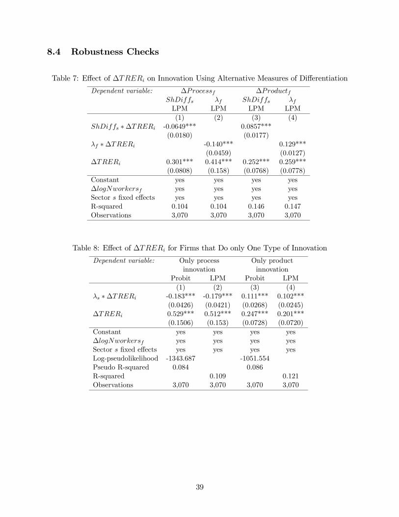
8.4 Robustness Checks
Table 7: E¤ect of �TRERi on Innovation Using Alternative Measures of Di¤erentiation
Dependent variable: �Processf �ProductfShDiffs �f ShDiffs �fLPM LPM LPM LPM(1) (2) (3) (4)
ShDiffs ��TRERi -0.0649*** 0.0857***(0.0180) (0.0177)
�f ��TRERi -0.140*** 0.129***(0.0459) (0.0127)
�TRERi 0.301*** 0.414*** 0.252*** 0.259***(0.0808) (0.158) (0.0768) (0.0778)
Constant yes yes yes yes�logNworkersf yes yes yes yesSector s �xed e¤ects yes yes yes yesR-squared 0.104 0.104 0.146 0.147Observations 3,070 3,070 3,070 3,070
Table 8: E¤ect of �TRERi for Firms that Do only One Type of Innovation
Dependent variable: Only process Only productinnovation innovation
Probit LPM Probit LPM(1) (2) (3) (4)
�s ��TRERi -0.183*** -0.179*** 0.111*** 0.102***(0.0426) (0.0421) (0.0268) (0.0245)
�TRERi 0.529*** 0.512*** 0.247*** 0.201***(0.1506) (0.153) (0.0728) (0.0720)
Constant yes yes yes yes�logNworkersf yes yes yes yesSector s �xed e¤ects yes yes yes yesLog-pseudolikelihood -1343.687 -1051.554Pseudo R-squared 0.084 0.086R-squared 0.109 0.121Observations 3,070 3,070 3,070 3,070
39
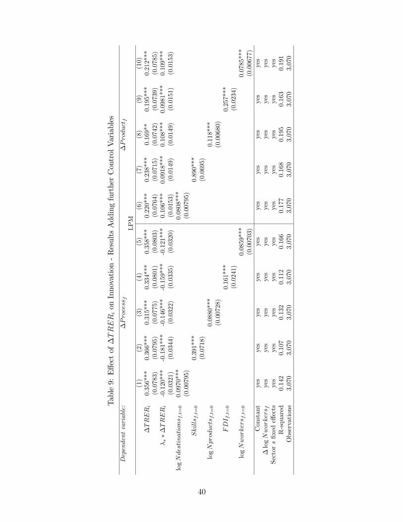
Table9:E¤ectof�TRERionInnovation-ResultsAddingfurtherControlVariables
Dependentvariable:
�Processf
�Productf
LPM
(1)
(2)
(3)
(4)
(5)
(6)
(7)
(8)
(9)
(10)
�TRERi
0.356***
0.366***
0.315***
0.334***
0.358***
0.220***
0.238***
0.169**
0.195***
0.212***
(0.0783)
(0.0795)
(0.0775)
(0.0801)
(0.0803)
(0.0764)
(0.0715)
(0.0742)
(0.0739)
(0.0785)
�s��TRERi
-0.120***
-0.181***
-0.146***
-0.159***
-0.121***
0.106***
0.0918***
0.108***
0.0981***
0.109***
(0.0321)
(0.0344)
(0.0322)
(0.0335)
(0.0320)
(0.0153)
(0.0149)
(0.0149)
(0.0151)
(0.0153)
logNdestinations f;t=0
0.0970***
0.0808***
(0.00795)
(0.00795)
Skillsf;t=0
0.391***
0.890***
(0.0718)
(0.0695)
logNproducts f;t=0
0.0880***
0.118***
(0.00728)
(0.00680)
FDI f;t=0
0.161***
0.257***
(0.0241)
(0.0234)
logNworkers f;t=0
0.0859***
0.0785***
(0.00703)
(0.00677)
Constant
yes
yes
yes
yes
yes
yes
yes
yes
yes
yes
�logNworkers f
yes
yes
yes
yes
yes
yes
yes
yes
yes
yes
Sectors�xede¤ects
yes
yes
yes
yes
yes
yes
yes
yes
yes
yes
R-squared
0.142
0.107
0.132
0.112
0.166
0.177
0.168
0.195
0.163
0.191
Observations
3,070
3,070
3,070
3,070
3,070
3,070
3,070
3,070
3,070
3,070
40

Table 10: E¤ect on Innovation Using Alternative Measures of TRERitLPM
Dependent variable: �Processf �Productf �Processf �Productf(1) (2) (3) (4)
�s ��TRERi;t�1 -0.118*** 0.0903***(0.0438) (0.0147)
�TRERi;t�1 0.295*** 0.194**(0.0829) (0.0901)
�s ��XTRERi -0.276*** 0.163***(0.0425) (0.0386)
�XTRERi 0.359*** 0.414***(0.0794) (0.158)
Constant yes yes yes yes� logNworkersf yes yes yes yesSector s �xed e¤ects yes yes yes yesR-squared 0.105 0.147 0.104 0.149Observations 3,041 3,041 3,070 3,070
Table 11: E¤ect of �TRERi on Innovation Using SURSUR 1 SUR 2
Dependent variable: �Processf �Productf �Processf �Productf(1) (2) (3) (4)
�s ��TRERi -0.124*** 0.106***(0.0334) (0.0155)
�TRERi 0.296*** 0.259*** 0.329*** 0.199**(0.0907) (0.0896) (0.0920) (0.0899)
Constant yes yes yes yes�logNworkersf yes yes yes yesSector s �xed e¤ects yes yes yes yesR-squared 0.104 0.146 0.107 0.149Observations 3,070 3,070 3,070 3,070
Table 12: Correlation between �s and Innovation Using World Bank Data for Brazil(1� e)s Process_WBf Product_WBf�s -0.0893 0.0105Notes: For the estimations we have used 1397 �rms for which we could combine �rm-level data with the
Khandelwal (2010) classi�cation of goods. The World Bank Survey for Brazil was conducted in year 2003.
41
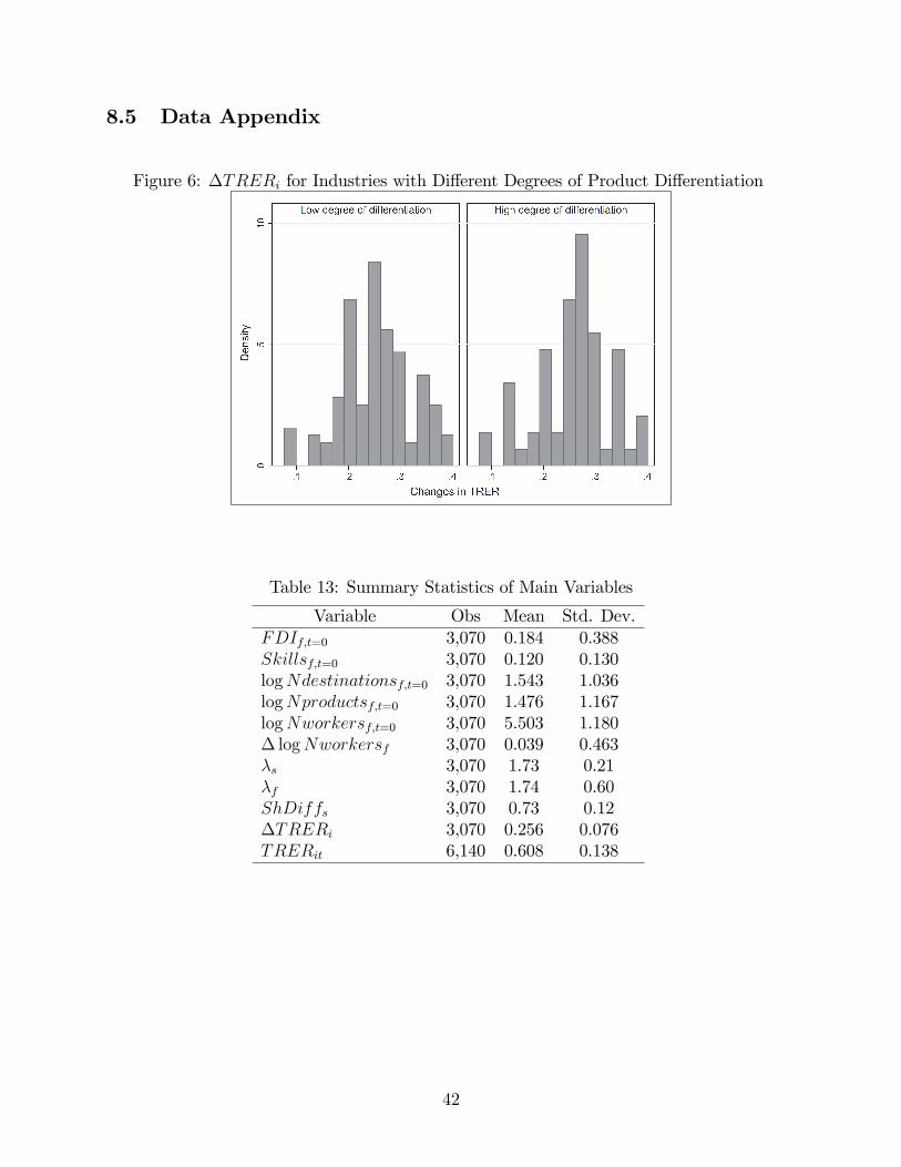
8.5 Data Appendix
Figure 6: �TRERi for Industries with Di¤erent Degrees of Product Di¤erentiation
Table 13: Summary Statistics of Main Variables
Variable Obs Mean Std. Dev.FDIf;t=0 3,070 0.184 0.388Skillsf;t=0 3,070 0.120 0.130logNdestinationsf;t=0 3,070 1.543 1.036logNproductsf;t=0 3,070 1.476 1.167logNworkersf;t=0 3,070 5.503 1.180� logNworkersf 3,070 0.039 0.463�s 3,070 1.73 0.21�f 3,070 1.74 0.60ShDiffs 3,070 0.73 0.12�TRERi 3,070 0.256 0.076TRERit 6,140 0.608 0.138
42
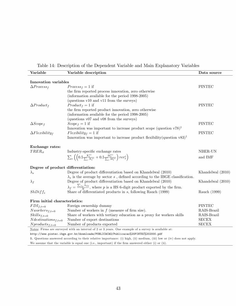
Table 14: Description of the Dependent Variable and Main Explanatory Variables
Variable Variable description Data source
Innovation variables�Processf Processf = 1 if PINTEC
the �rm reported process innovation, zero otherwise(information available for the period 1998-2005)(questions v10 and v11 from the surveys)
�Productf Productf = 1 if PINTECthe �rm reported product innovation, zero otherwise(information available for the period 1998-2005)(questions v07 and v08 from the surveys)
�Scopef Scopef = 1 if PINTECInnovation was important to increase product scope (question v78)1
�Flexibilityf Flexibilityf = 1 if PINTECInnovation was important to increase product �exibility(question v83)1
Exchange rates:TRERit Industry-speci�c exchange rates NBER-UNP
c
��0:5
XsctP
cXsct+ 0:5
MsctP
cMsct
�rerct
�and IMF
Degree of product di¤erentiation:�s Degree of product di¤erentiation based on Khandelwal (2010) Khandelwal (2010)
�s is the average by sector s , de�ned according to the IBGE classi�cation.�f Degree of product di¤erentiation based on Khandelwal (2010) Khandelwal (2010)
�f =P
fp �fpN , where p is a HS 6-digit product exported by the �rm.
ShDiffs Share of di¤erentiated products in s, following Rauch (1999) Rauch (1999)
Firm initial characteristics:FDIf;t=0 Foreign ownership dummy PINTECNworkersf;t=0 Number of workers in f (measure of �rm size). RAIS-BrazilSkillsf;t=0 Share of workers with tertiary education as a proxy for workers skills RAIS-BrazilNdestinationsf;t=0 Number of export destinations SECEXNproductsf;t=0 Number of products exported SECEXNotes: Firms are surveyed with an interval of 2 or 3 years. One example of a survey is available at:
http://www.pintec.ibge.gov.br/downloads/PUBLICACAO/Publicacao%20PINTEC%202000.pdf
1. Questions answered according to their relative importance: (i) high, (ii) medium, (iii) low or (iv) does not apply.We assume that the variable is equal one (i.e., important) if the �rm answered either (i) or (ii).
43


