empirical essays on fiscal federalism and political ... · gäbler, björn kauder, and martin...
TRANSCRIPT

842019
Empirical essays on fiscal federalism and political economy in GermanyManuela Maria Krause

Bibliografische Information der Deutschen Nationalbibliothek Die Deutsche Nationalbibliothek verzeichnet diese Publikation in der Deutschen Nationalbibliografie; detaillierte bibliografische Daten sind im Internet über http://dnb.d-nb.de abrufbar. ISBN: 978-3-95942-061-7 Alle Rechte, insbesondere das der Übersetzung in fremde Sprachen, vorbehalten. Ohne ausdrückliche Genehmigung des Verlags ist es auch nicht gestattet, dieses Buch oder Teile daraus auf photomechanischem Wege (Photokopie, Mikrokopie) oder auf andere Art zu vervielfältigen. © ifo Institut, München 2019 Druck: ifo Institut, München ifo Institut im Internet: http://www.cesifo-group.de

Herausgeber der Reihe: Clemens FuestSchriftleitung: Chang Woon Nam
Empirical essays on fiscal federalism and political economy in Germany Manuela Maria Krause
842019
i
Acknowledgments
First and foremost, I would like to thank my first supervisor, Niklas Potrafke, for his guidance
and support throughout all stages of this thesis. His encouragement and helpful comments
were always a source of inspiration for me. I also want to thank Thiess Büttner as my second
supervisor for his support and valuable comments on my research ideas. I learned much from
both – especially in the joint research projects – which also broadened my horizons. I am also
grateful to Andreas Haufler for agreeing to be my third supervisor.
I further want to thank my colleagues Johannes Blum, Luisa Dörr, Florian Dorn, Stefanie
Gäbler, Björn Kauder, and Martin Mosler for their support, the fruitful and interesting discus-
sions as well as the pleasant lunch and coffee breaks. I enjoyed our joint trips and our confer-
ence stays at various cities in the world. I am especially thankful to Luisa and Stefanie for our
talks, the daily coffee breaks in the morning, the muffins, their extensive moral support and
their friendship. I also would like to thank all my former colleagues, with whom I shared my
first experiences in academia – Kai Jäger, Markus Reischmann, Marina Riem, and Christoph
Schinke.
Interns, research assistants and the administrative staff at the ifo Institute provided me with
helpful support during the entire time. Among many others, I am especially grateful to Kristin
Fischer and Alexander H. Schwemmer for their excellent research assistance and helpful sug-
gestions for my own work and for the third-party projects.
Completing this thesis would not have been possible without the help of my family and
friends. I especially want to thank my parents for their endless support, encouragement, love
and the regular parcels with chocolate and other sweets – especially in the last weeks while
finishing this thesis. Last but not least, I thank Björn for his love, his comprehensive support,
his incredible patience and for being there for me whenever I need it.

Empirical essays on fiscal federalism and
political economy in Germany
Inaugural-Dissertation
zur Erlangung des Grades
Doctor oeconomiae publicae (Dr. oec. publ.)
an der Ludwig-Maximilians-Universität München
2018
vorgelegt von:
Manuela Maria Krause
Referent: Prof. Dr. Niklas Potrafke
Korreferent: Prof. Dr. Thiess Büttner
Promotionsabschlussberatung: 30. Januar 2019

Datum der mündlichen Prüfung: 23.01.2019
Namen der Berichterstatter: Prof. Dr. Niklas Potrafke
Prof. Dr. Thiess Büttner
Prof. Dr. Andreas Haufler
v
Content
1 Introduction ..................................................................................................... 1
References .............................................................................................................................. 9
2 Communal fees and election cycles: Evidence from German municipalities ........... 11
Introduction ................................................................................................................ 12
Related literature ........................................................................................................ 13
Institutional backdrop ................................................................................................ 15
2.3.1 German municipalities ................................................................................... 15
2.3.2 Municipal elections ......................................................................................... 16
Data and methodology ............................................................................................... 17
2.4.1 Data sources ................................................................................................... 17
2.4.2 Empirical strategy ........................................................................................... 18
Regression results ....................................................................................................... 19
2.5.1 Baseline results ............................................................................................... 19
2.5.2 Robustness tests ............................................................................................. 21
Conclusion ................................................................................................................... 24
References ............................................................................................................................ 26
Appendix ............................................................................................................................... 31
3 Electoral cycles in MPs‘ salaries: Evidence from the German states ...................... 39
Introduction ................................................................................................................ 40
Institutional backdrop ................................................................................................ 42
3.2.1 MP salaries in the German states ................................................................... 42
3.2.2 State elections ................................................................................................ 42
Empirical analysis ....................................................................................................... 43
3.3.1 Descriptive statistics ....................................................................................... 43
3.3.2 Empirical strategy ........................................................................................... 44
3.3.3 Regression results ........................................................................................... 45
3.3.4 Robustness tests ............................................................................................. 46
Conclusion ................................................................................................................... 48
References ............................................................................................................................ 50
vi
Appendix ............................................................................................................................... 56
4 Do left-wing governments decrease income inequality? Empirical evidence based
on salaries of civil servants .............................................................................. 67
Introduction ................................................................................................................ 68
Background and hypothesis ....................................................................................... 68
4.2.1 Government ideology and income redistribution ......................................... 68
4.2.2 Ideology-induced policies in the German states ........................................... 70
Institutional backdrop ................................................................................................ 71
4.3.1 Salaries of civil servants ................................................................................. 71
4.3.2 The German political party landscape........................................................... 71
Empirical analysis ....................................................................................................... 72
4.4.1 Empirical strategy ........................................................................................... 72
4.4.2 Descriptive statistics ....................................................................................... 74
4.4.3 Regression results ........................................................................................... 74
4.4.4 Robustness tests ............................................................................................. 75
Salaries of cabinet members ...................................................................................... 76
Conclusion ................................................................................................................... 77
References ............................................................................................................................ 78
Appendix ............................................................................................................................... 81
5 The real-estate transfer tax and government ideology: Evidence from the
German states ................................................................................................ 89
Introduction ................................................................................................................ 90
Institutional background ............................................................................................ 92
5.2.1 State governments in Germany’s federalism ................................................ 92
5.2.2 The German real-estate transfer tax .............................................................. 93
Case study evidence ................................................................................................... 93
Empirical analysis ....................................................................................................... 95
5.4.1 Unconditional correlations ............................................................................ 95
5.4.2 Conditional correlations................................................................................. 97
5.4.3 Robustness tests ............................................................................................. 98
Conclusion ................................................................................................................. 100
References .......................................................................................................................... 102
vii
Appendix ............................................................................................................................. 105
6 Federalism in Wonderland: Tax autonomy in German real-estate transfer
taxation ...................................................................................................... 119
Introduction .............................................................................................................. 120
Tax autonomy and fiscal equalization ..................................................................... 122
Definition of the marginal retention rate ................................................................. 123
Simulation of the marginal retention rate ............................................................... 125
The development of the marginal retention rate .................................................... 126
Conclusion ................................................................................................................. 129
References ......................................................................................................................... 131
Appendix ............................................................................................................................ 132
7 Fiscal equalization as a driver of tax increases: Empirical evidence from
Germany ..................................................................................................... 139
Introduction .............................................................................................................. 140
Tax policy under fiscal equalization ......................................................................... 142
Empirical methodology ............................................................................................ 145
Data ........................................................................................................................... 147
7.4.1 Fiscal equalization in Germany .................................................................... 147
7.4.2 Descriptive statistics ..................................................................................... 149
Results ....................................................................................................................... 150
Summary and conclusions ....................................................................................... 151
References .......................................................................................................................... 153
Appendix ............................................................................................................................. 155
A Data sources and definitions........................................................................ 155
B Tables and Figures ........................................................................................ 157
8 Conclusion ................................................................................................... 167
Curriculum Vitae ................................................................................................ 171

ix
List of figures
Figure 1.1: Municipal revenues by different sources, 1992–2015 ............................................... 4
Figure 1.2: States’ expenditures by type of expenditure, 2011 ................................................... 5
Figure 1.3: Average tax rate and tax revenues of the real-estate transfer tax, 2006–2016 ........ 7
Figure 2.1: Average revenues from utilization fees in per-capita terms, 1992–2006 ............... 31
Figure 2.2: Average change in per-capita fees by election year variables ............................... 32
Figure 3.1: Average increase in MP salaries by election period dummies ................................ 56
Figure 3.2: Average increase in MP salaries by share of legislative period passed .................. 57
Figure 3.3: Average increase in MP and employee salaries, 1980–2014 ................................... 58
Figure 4.1: Increases in inequality of civil servants’ salaries by type of government .............. 81
Figure 5.1: Increases in the real-estate transfer tax rate by type of government,
2007–2017 ................................................................................................................................. 105
Figure 5.2: Real-estate transfer tax rate by type of government, 2007–2017 ........................ 106
Figure 5.3: Increases in the real-estate transfer tax rate by type of government,
West German states, 2007–2017 .............................................................................................. 107
Figure 5.4: Real-estate transfer tax rate by type of government, West German states,
2007–2017 ................................................................................................................................. 108
Figure 5.5: Increases in the real-estate transfer tax rate by type of government,
East German states, 2007–2017 ............................................................................................... 109
Figure 5.6: Real-estate transfer tax rate by type of government, East German states,
2007–2017 ................................................................................................................................. 110
Figure 5.7: Conditional correlations – real-estate transfer tax rate by type of government,
2007–2017 (I) ............................................................................................................................. 115
Figure 5.8: Conditional correlations – real-estate transfer tax rate by type of government,
2007–2017 (II) ............................................................................................................................ 117
Figure 6.1: Representative tax rate and average marginal retention rate ............................. 134
Figure 6.2: Marginal retention rates for group 1, 2006–2016 .................................................. 135
Figure 6.3: Marginal retention rates for group 2, 2006–2016 .................................................. 136
Figure 6.4: Marginal retention rates for group 3, 2006–2016 .................................................. 137
Figure 7.1: Real-estate transfer tax rate increases among the German states ...................... 157
Figure 7.2: Equalization transfers and relative fiscal capacity ............................................... 158
Figure 7.3: Degree of fiscal redistribution (tax base 𝛽), 2006–2016 ....................................... 160
Figure 7.4: Degree of fiscal redistribution (tax base 𝛽), counterfactual simulations,
2006–2016 ................................................................................................................................. 161

xi
List of tables
Table 2.1: Descriptive statistics ................................................................................................. 33
Table 2.2: Correlation between the main variables .................................................................. 34
Table 2.3: Local election dates .................................................................................................. 34
Table 2.4: OLS regression results ............................................................................................... 35
Table 2.5: OLS regression results for subcategories ................................................................. 36
Table 2.6: GMM results ............................................................................................................... 37
Table 3.1: Descriptive statistics ................................................................................................. 59
Table 3.2: Correlation between the main variables .................................................................. 59
Table 3.3: OLS regression results with election period dummies (I) ........................................ 60
Table 3.4: OLS regression results with election period dummies (II) ....................................... 61
Table 3.5: OLS regression results with continuous time variable (I) ........................................ 62
Table 3.6: OLS regression results with continuous time variable (II) ....................................... 63
Table 3.7: OLS regression results including indexed years ....................................................... 64
Table 3.8: OLS regression results for indexed years ................................................................. 65
Table 4.1: Example of a salary scale, North Rhine-Westphalia 2012 ........................................ 82
Table 4.2: Descriptive statistics ................................................................................................. 83
Table 4.3: Correlation between the main variables .................................................................. 84
Table 4.4: OLS regression results with categorical government ideology variable (I) ............ 85
Table 4.5: OLS regression results with categorical government ideology variable (II) ........... 86
Table 4.6: OLS regression results with ideology dummies ....................................................... 87
Table 4.7: Percentage premia for cabinet members in the German states ............................. 88
Table 5.1: Real-estate transfer tax rate by states and type of government, 2007–2017 ....... 111
Table 5.2: Descriptive statistics ............................................................................................... 112
Table 5.3: Correlation between the main variables ................................................................ 113
Table 5.4: OLS regression results (I)......................................................................................... 114
Table 5.5: OLS regression results (II) ....................................................................................... 116
Table 6.1: Real-estate transfer tax rates, 2006–2016 .............................................................. 132
Table 6.2: Marginal retention rates of the states in 2006 and 2016 ........................................ 133
Table 7.1: Fiscal redistribution by state in 2006 and 2016 ...................................................... 159
Table 7.2: Descriptive statistics ............................................................................................... 162
Table 7.3: OLS regression results ............................................................................................. 163
Table 7.4: IV regression results ................................................................................................ 164
Table 7.5: IV regression results including the equalization rate effect .................................. 165
Table 7.6: IV regression results including state debt .............................................................. 166

Introduction
1
1 Introduction
“There can be no doubt, that if power is granted to a body of men,
called representatives,
they, like any other men, will use their power, not for the advantage of the community,
but for their own advantage, if they can.”
(James Mill)
In many countries, governments have been decentralized to improve the performance of the
public sector. The main question to answer is how to align tasks and policy instruments
among the different levels of government. This is the subject of fiscal federalism. Main contri-
butions to this theory were made by Tiebout (1956), Musgrave (1959) or Oates (1972).1 The
idea is that decentralization can increase economic welfare. Decentralized governments can
better cater heterogeneous interests than a centralized government. Oates (1972) emphasizes
that for the efficient provision of public utilities, the services should be provided by the lowest
possible level representing the area where citizens demand these services. Combined with the
traditional model of revealed preferences by Tiebout (1956), a decentralized provision of pub-
lic services can thus give rise to a pareto optimal provision of the services (Darby et al. 2003).
The idea of decentralization is typically realized by implementing a federal system, consisting
of different levels of governments. Each level is responsible for individual tasks and has to
provide specific public services. A federal system requires however also appropriate fiscal in-
struments for each level to fulfill these tasks (Oates 1999). Federal systems are thus typically
characterized by fiscal autonomy for the different levels of governments. Fiscal autonomy in-
cludes deciding on expenditures, as already stated by Oates (1972), and also imposing taxes
or using (to a limited extent) debt instruments. Autonomy can however induce externalities
and disparities between subnational regions.2 Many federations thus implemented intergov-
ernmental grants or systems of equalization to reduce possible disparities (Buchanan 1950,
1952).3 Equalization grants can however also provide incentives and – particularly in combi-
nation with tax autonomy – give rise to distortions (Oates 2005). Equalization grants may, for
example, reduce efforts to generate own revenues. The exact institutional design of federal
systems thus plays an important role.
1 For an overview, see Oates (1999).
2 Gordon (1983) shows that decentralized tax and expenditure policies can give rise to inefficiencies in the economic activity.
3 For an introduction in the theory of equalization, see Boadway (2004).
Introduction
2
The literature on fiscal federalism has been extended by several fields and disciplines over
time.4 One important strand relates to the field of public choice and political economy. The
early contributions to the theory of fiscal federalism have assumed that politicians and public
officials are benevolent and maximize social welfare (Oates 1972). The theory of public choice,
by contrast, assumes that politicians have self-interests and act to maximize their own welfare
(Downs 1957, Buchanan and Tullock 1962). Contributions to this literature thus investigate
political processes and how political agents behave.5
One strand of the literature stresses the importance of elections. The political business cycle
theories describe that politicians have an incentive to increase their reelection chances by
pursuing expansionary policies before elections to influence the level of economic activity.
The first contributions to this literature by Nordhaus (1975) and MacRae (1977) proposed the-
oretical models based on a Phillips curve tradeoff between inflation and unemployment. Ac-
cording to these models, politicians will inflate more during election years – by expansionary
monetary and fiscal policies. These policies will give rise to a lower unemployment rate and
thus to a favorable situation for the incumbent politicians. Although this theory received great
attention, a shortcoming of these models was the assumption of adaptive voter expectations,
i.e., voters form their expectations based on what has happened in the past. Following contri-
butions thus developed models of political business cycles under rational voter expectations
(Rogoff and Sibert 1988, Rogoff 1990). Many studies have explored the theory of political busi-
ness cycles empirically. Early contributions have focused on macroeconomic outcome varia-
bles such as unemployment and inflation. More recent studies have examined political busi-
ness cycles in variables such as debt, expenditures or revenues of governments.
A second strand within the theory of public choice and an extension of the political business
cycle theories points to the importance of parties and their ideologies for economic policy-
making (Hibbs 1977). The partisan theories describe that politicians from different parties –
mostly divided into left-wing and right-wing parties – will pursue different policies in line with
the preferences of their constituencies. The theory is also based on the Phillips curve tradeoff
described above. Left-wing voters are assumed to be blue-collar workers, while right-wing
voters are mostly capital owners with higher income. Left-wing parties, who gratify the needs
of their voters, will thus favor low unemployment rates and accept higher inflation rates.
Right-wing parties will in contrast favor lower inflation rates while accepting higher unem-
ployment rates. Left-wing parties thus pursue more expansionary policies than right-wing
parties. The partisan approach was also extended by rational expectations (Chappell and
4 Extensions to the literature on fiscal federalism by other fields and disciplines are often called “The second-generation theory
of fiscal federalism”, see, e.g., Oates (2005) or Weingast (2009).
5 For a comprehensive introduction, see Mueller (2003).
Introduction
3
Keech 1986, Alesina 1987). Many empirical studies have investigated whether government ide-
ology influences economic policy-making.6
This thesis elaborates on selected incentives in fiscal federalism using the example of the fed-
eral system in Germany. As described above, depending on the exact implementation, fiscal
federalism per se can provide fiscal incentives. In addition, combined with public choice the-
ories, also political incentives are possible. The main part of this thesis examines political in-
centives within Germany’s federalism, while the last two chapters also investigate fiscal in-
centives stemming from the exact design of federalism in Germany. The thesis takes a reform
of the fiscal constitution in 2006 into account, which realigned legislative powers between the
different levels of government. The reform aimed to decentralize financial responsibilities and
to improve the efficiency within the federal system by granting the states some new rights.
The German federal system consists of three tiers: the federal level, the states and the munic-
ipalities.7 All levels have different rights and duties but are also linked to each other for specific
tasks. In Germany’s federalism, the subsidiarity principle is implemented. The states and the
municipalities have to fulfill a plethora of tasks. Both levels are in general also responsible for
financing their tasks as the administrative and financial responsibility are linked according to
the constitution (Konnexitätsprinzip). State and municipal governments have various revenue
sources to finance their tasks. Tax revenues are the most important source for both levels. In
specific cases, the federal or state governments also support the subnational governments in
financing their tasks. Important are also the equalization schemes, which aim to equalize
funds between the subnational levels. The degree of discretion, i.e., the fiscal autonomy, of
states and municipalities varies however over these resources.
Chapter 2 focuses on municipalities. The German municipalities have various revenue
sources. The largest part consists of shared taxes, over which the municipalities have only
limited influence. Municipalities may however set the tax rates of local taxes. The municipali-
ties also receive equalization grants from the communal equalization schemes. The federal or
state level also grants financial contributions for supplying certain public services. Another
important source of municipalities’ revenues are fees, which are levied for the effective use of
a public service. Municipalities can decide independently of other governmental tiers on the
fees of most public services. Municipalities thus have fiscal autonomy over fees.
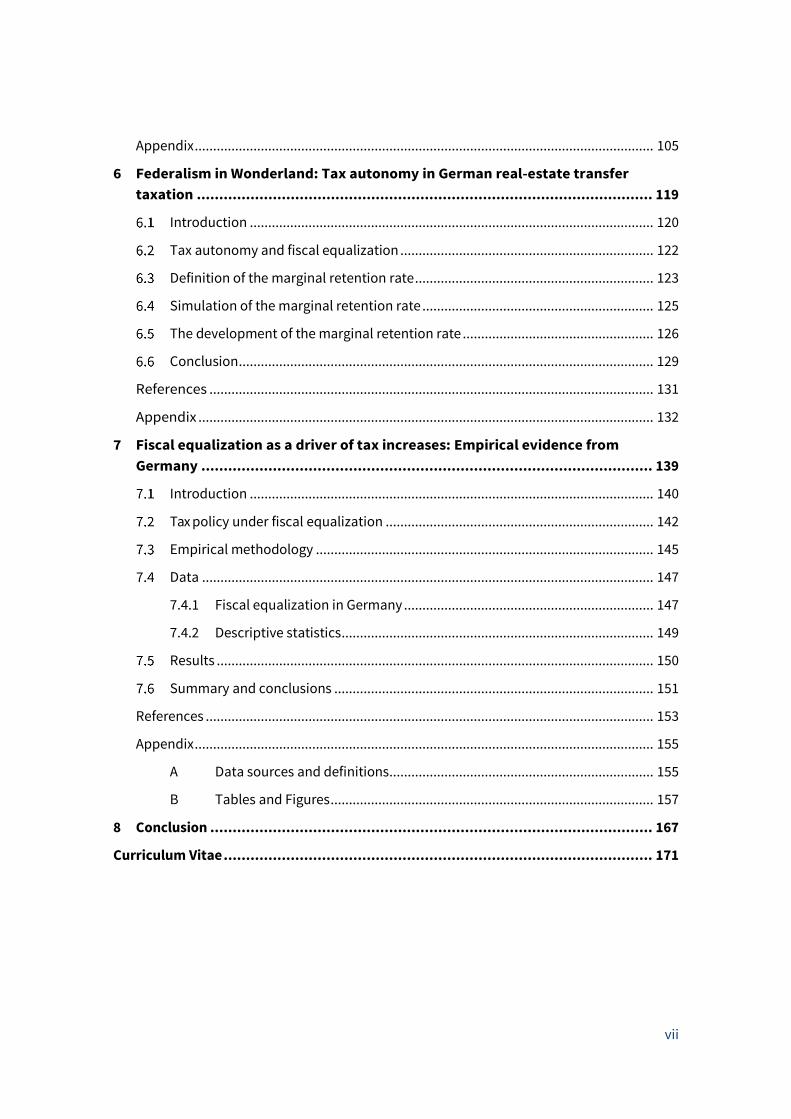
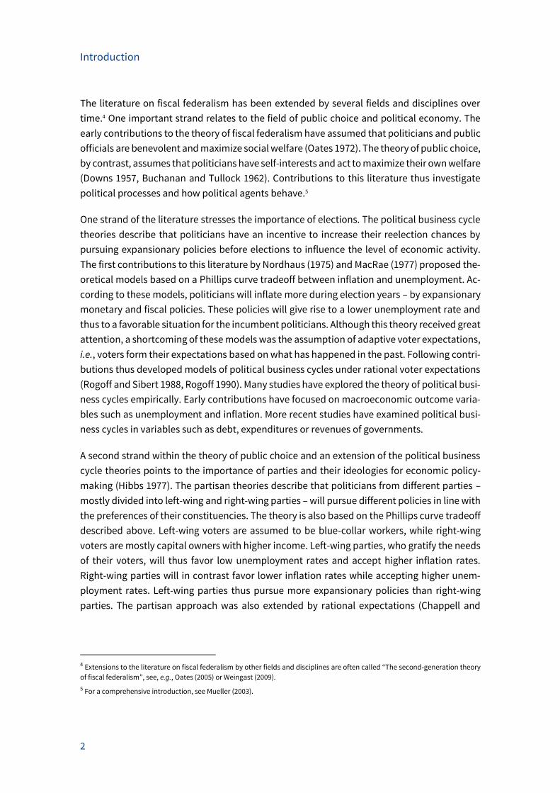
Figure 1.1 shows the average development of tax revenues, financial grants and fees as a share
of overall revenues for municipalities of the West German states in the time period from 1992
to 2015.8 After tax revenues and grants, fees are the third most important revenue category
6 For a survey on OECD panel studies, see Potrafke (2017).
7 An introduction in the federal system in Germany is provided by Blankart (2011) and Brümmerhoff and Büttner (2015).
8 The sample includes municipalities from Baden-Wuerttemberg, Bavaria, Hesse, Lower Saxony, North Rhine-Westphalia, Rhine-
land-Palatinate, Saarland and Schleswig-Holstein. The city states Hamburg and Bremen are excluded.
Introduction
4
for the municipalities. The share of revenues from fees accounts on average for 12 percent of
overall revenues. The share has declined over time with a short-time increase in 2011. In 2015,
fees accounted again for 12 percent of overall municipal revenues.
Figure 1.1: Municipal revenues by different sources, 1992–2015
Source: Statistisches Bundesamt (different years); own illustration.
Communal fees are thus an important revenue source for German municipalities. Fees should
be equivalent to the (expected) costs of public services and thus represent the benefit princi-
ple in public finance. The local councils of municipalities, which are by law responsible for
setting fees, have however a leeway to determine fees. In Chapter 2, I examine this leeway by
elaborating whether electoral cycles, based on the political business cycle theories by
Nordhaus (1975) and Rogoff (1990), occur in communal fees of German municipalities. I use
revenue data for around 7,000 West German municipalities from seven states over the period
1992–2006. The results show that municipalities increase communal fees less in election years
than in the middle of the legislative period, while they increase fees more directly after elec-
tions. Fees increase in election years by 0.94 euro per capita less than in the middle of the
legislative period. Fees increase however directly after an election by about 1.74 euro per cap-
ita more than in the middle of the legislative period. This behavior is consistent with the pre-
dictions of the political business cycle theories.
The following chapters of this thesis focus on the state level in Germany. The states also have
to fulfill important tasks. The link between the administrative and financial responsibility pro-
vides the states in general with the possibility to decide on their expenditures. The degree of
Introduction
5
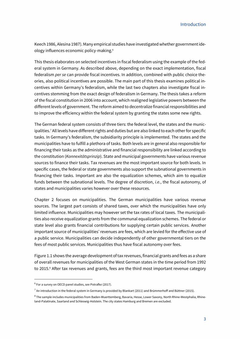
discretion varies however between different expenditure categories (e.g., Seitz 2008). A large
part of the expenditures consists of personnel expenditures. Figure 1.2 shows for the year 2011
the states’ expenditures for different types of public expenditure as a share of overall current
expenditures. Personnel expenditures account for the largest share. Nearly 40 percent of all
current expenditures are for personnel costs. An interesting subcategory of the personnel ex-
penditures are expenditures for members of parliament (MP) and for civil servants. Since a
decision of the Supreme Court in 1975, the German states have a leeway to decide on MP sal-
aries. Salary adjustments of MPs however often cause disenchantment of voters with politics.
The given leeway may thus provide incentives for politicians, who aim to reward their constit-
uencies. In line with the political business cycle theories, politicians may reschedule salary
increases of their own salaries because of elections.
Figure 1.2: States’ expenditures by type of expenditure, 2011
Note: Expenditures are calculated as the shares of overall expenditures according to
current accounts.
Source: Statistisches Bundesamt (2011); own illustration.
In Chapter 3, which is joint work with Björn Kauder and Niklas Potrafke (based on Kauder et
al. 2018), we investigate electoral cycles in salary increases of German state MPs. We use data
for 15 states over the period from 1980 to 2014. The results do not show that elections influ-
ence increases in MP salaries. Politicians can increase MPs’ salaries at any point in time with-
out suffering from negative consequences.
Introduction
6
Politicians may however not only influence policies because of reelection concerns. As de-
scribed above, government ideology may also predict economic policy-making. For the Ger-
man states, many studies provide evidence that government ideology influences individual
policy fields.9 In some policy fields, however, the states have no discretion to decide inde-
pendently on the policies. A reform of the German fiscal constitution in 2006 restructured leg-
islative powers between the federal and the state governments. Among other changes, the
reform allowed the states to design discretionarily the salaries of their civil servants. Before
the reform, the federal level held the decision power on the salaries of all civil servants in all
states. Civil servants reflect a large share in the public sector in Germany and include different
professions, for example servants in the administration, professors or judges. Their salaries
differ considerably. Salaries of civil servants may thus serve as a proxy for the income distri-
bution within the public sector. Government ideology has been shown to influence redistribu-
tion of income (e.g., Scheve and Stavasage 2009). Left-wing governments redistribute income
from high-income citizens to low-income citizens, thus reducing income inequality. Right-
wing governments are not expected to redistribute as much as left-wing governments. The
given leeway in deciding on salaries of civil servants may also give state governments, influ-
enced by their ideology, the opportunity to redistribute income between different groups of
civil servants.
In Chapter 4, which is again joint work with Björn Kauder and Niklas Potrafke, we investigate
whether government ideology influences redistribution of income within the public sector of
the German states. We use data on salaries of civil servants in the states since 2007. The hy-
pothesis to be tested is that left-wing governments redistribute income from high-income civil
servants to low-income civil servants, thus reducing income inequality within the public sec-
tor more than right-wing governments. We use five income inequality measures comparing
salaries across pay levels and operating experiences of different groups of civil servants. The
results do not show that left-wing governments were more active in decreasing income ine-
quality among civil servants than center or right-wing governments.
Another key element of the federal reform in 2006 was the devolution of tax setting powers to
the states. Before the reform, the states had for a long time no discretion over own tax instru-
ments. The states have in general various revenue sources, but the degree of discretion, i.e.,
their fiscal autonomy, varies over the sources. The main part of states’ revenues consists of
shared taxes, over which individual states have no discretion to influence the tax rates. Be-
sides shared taxes, the states also obtain revenues from state taxes, whose amounts are ex-
clusively for the states. The most important state taxes – in revenue terms – are the real-estate
transfer tax and the inheritance tax. The reform in 2006 allowed the states to set the tax rates
of the real-estate transfer tax. The states thus received after a long time again tax autonomy
for an individual tax. After the reform in 2006, many states began to increase their tax rates.
9 For an overview, see Section 4.2.2.
Introduction
7
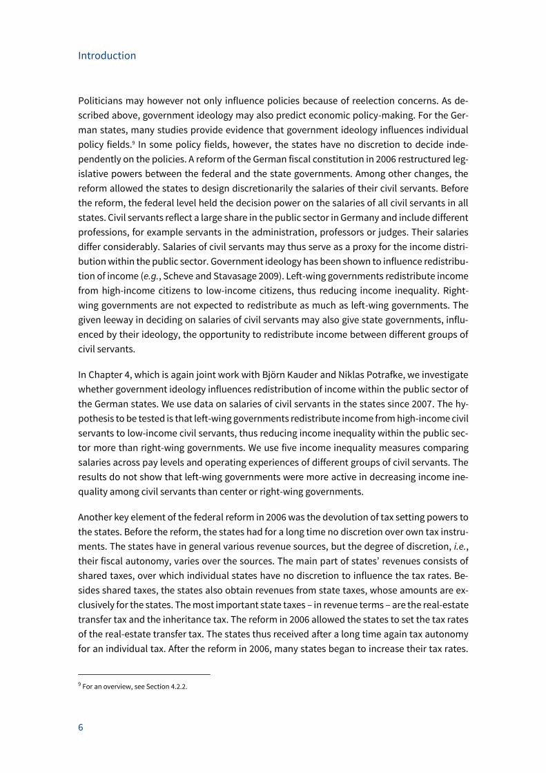
No state lowered its tax rate. Figure 1.3 shows the average development in tax rates and in tax
revenues (in per-capita terms) among all 16 states since 2006. The averages of tax rates and
revenues have increased considerably over time. Before the reform, the tax rate was fixed at
a level of 3.5 percent for all states. In 2016, the mean tax rate reached a level of 5.3 percent.
Per-capita revenues from the real-estate transfer tax have also increased considerably over
time.
Figure 1.3: Average tax rate and tax revenues of the real-estate transfer tax, 2006–2016
Note: Average of real-estate transfer tax rates among the 16 states and average of reve-
nues from the real-estate transfer tax in per-capita terms.
Source: State announcements and Federal Ministry of Finance; own illustration.
The real-estate transfer tax has to be paid on the sale price of the real estate determined in a
contract between the selling and the purchasing party. Although tax rates do not seem to be
very high, the amount to be paid by the buyer of a real estate is usually quite high because of
the sizeable tax base. Among all transaction costs, which have to be paid for purchasing real
estate, the real-estate transfer tax accounts in Germany for more than 50 percent (Andrews et
al. 2011).10 The tax is thus not neglectable for citizens.
In Chapter 5, which is joint work with Niklas Potrafke (based on Krause and Potrafke 2017),
we investigate whether government ideology predicts tax rates of the real-estate transfer tax.
10 Transaction costs include in general real-estate transfer taxes, notary and legal fees, registration fees and real-estate agent
fees (Andrews et al. 2011).
Introduction
8
Since the real-estate transfer tax is likely to influence high-income citizens, who often own
property, right-wing and left-wing governments may well differ in their tax policy because of
diverging interests of their constituencies. We investigate increases in the tax rates of all 16
German states for the period from 2007 to 2017. Our descriptive results show that left-wing
and center governments were more active in increasing the tax rates of the real-estate trans-
fer tax than right-wing governments. The results of the empirical analysis show that – condi-
tional on other explanatory variables – the real-estate transfer tax rate is 0.52 percentage
points higher under left-wing than under right-wing governments. The results thus indicate
that political parties, when given the opportunity, are prepared to offer polarized tax policies.
Besides revenues from taxes, the fiscal equalization scheme is another important revenue
source for the German states. The German fiscal equalization scheme aims at equalizing funds
available for the states to ensure equal conditions in every state. The equalization scheme
consists of different horizontal and vertical stages, which redistribute revenues among the
federal and state level and between the states. The devolution of tax setting powers to the
states with the federal reform in 2006 provides an interesting set-up to investigate. The com-
bination of tax autonomy and fiscal equalization may provide distortions (Oates 2005). Equal-
ization schemes may, for example, provide fiscal incentives to reduce own tax efforts (Mus-
grave 1959).
In Chapters 6 and 7, which are both joint work with Thiess Buettner (Chapter 6 is based on
Buettner and Krause 2018), we thus investigate whether also the German fiscal equalization
scheme influences the states’ real-estate transfer tax policy. In the German case, the revenues
of the real-estate transfer tax are used within the equalization system. We use a simulation
model of the fiscal equalization scheme to calculate the degree of redistribution of tax reve-
nues from real-estate transfer taxes within the equalization scheme. We use data for the pe-
riod from 2006 to 2016 in Chapter 6 and from 2006 to 2017 in Chapter 7. The descriptive results
in Chapter 6 and the empirical analysis in Chapter 7 show that the substantial redistribution
of revenues from the real-estate transfer tax within fiscal equalization provides significant in-
centives for the states to raise their tax rates. With full equalization, a state is predicted to set
the tax rate of the real-estate transfer tax about 1.3 percentage points higher than without.
The results show further that the incentive effect to raise the tax rate is even proliferated by
the equalization scheme. Equalization thus substantially influences tax policies of the states.
In this thesis, I thus examine several political and fiscal incentives within Germany’s federal
system providing new and interesting results. Some of the results may be relevant for policy-
makers or for upcoming debates about the federal system in Germany.
Introduction
9
References
Alesina, A. (1987). Macroeconomic policy in a two-party system as a repeated game. Quarterly
Journal of Economics, 102, 651–678.
Andrews, D., A. C. Sanchez, and A. Joansson (2011). Housing market and structural policies in
OECD countries. OECD Economics Department Working Paper 836.
Blankart, C. B. (2011). Öffentliche Finanzen in der Demokratie. 8th edition, München: Verlag
Franz Vahlen.
Boadway, R. (2004). The theory and practice of equalization. CESifo Economic Studies, 50(1),
211–254.
Brümmerhoff, D. and T. Büttner (2015). Finanzwissenschaft. 11th edition, Oldenburg: de Gruy-
ter.
Buchanan, J. M. (1950). Federalism and fiscal equity. American Economic Review, 40, 583–599.
Buchanan, J. M. (1952). Central grants and resource allocation. Journal of Political Economy,
60, 208–217.
Buchanan, J. M. and G. Tullock (1962). The Calculus of Consent: The Logical Foundations of Con-
stitutional Democracy. Ann Arbor: University of Michigan Press.
Buettner, T. and M. Krause (2018). Föderalismus im Wunderland: Zur Steuerautonomie bei der
Grunderwerbsteuer. Perspektiven der Wirtschaftspolitik, 19(1), 32–41.
Chappell, H. W. Jr. and W. R. Keech (1986). Party differences in macroeconomic policies and
outcomes. American Economic Review, 76, 71–74.
Darby, J., A. V. Muscatelli, and G. Roy (2003). Fiscal decentralization in Europe: A review of re-
cent experience. European Research in Regional Science, 13, 1–32.
Downs, A. (1957). An Economic Theory of Democracy. New York: Harper and Row.
Gordon, R. H. (1983). An optimal taxation approach to fiscal federalism. Quarterly Journal of
Economics, 98(4), 567–586.
Hibbs, D. A. Jr. (1977). Political parties and macroeconomic policy. American Political Science
Review, 71, 1467–1487.
Kauder, B., M. Krause and N. Potrafke (2018). Electoral cycles in MPs’ salaries: Evidence from
the German states. International Tax and Public Finance, 25, 981–1000.
Krause, M. and N. Potrafke (2017). The real-estate transfer tax and government ideology: Evi-
dence from the German states. CESifo Working Paper 6491.
MacRae, D. (1977). A political model of the business cycle. Journal of Political Economy, 85,
239–263.
Mueller, D. C. (2003). Public choice III. 3rd edition, New York: Cambridge University Press.
Introduction
10
Nordhaus, W. D. (1975). The political business cycle. Review of Economic Studies, 42, 169–190.
Musgrave, R. (1959). The Theory of Public Finance. New York: McGraw-Hill.
Oates, W. E. (1972). Fiscal Federalism. New York: Harcourt Brace Jovanovich.
Oates, W. E. (1999). An essay on fiscal federalism. Journal of Economic Literature, 37, 1120–
1149.
Oates, W. E. (2005). Toward a second-generation theory of fiscal federalism. International Tax
and Public Finance, 12, 349–373.
Potrafke, N. (2017). Partisan politics: The empirical evidence from OECD panel studies. Jour-
nal of Comparative Economics, 45, 712–750.
Rogoff, K. (1990). Equilibrium political budget cycles. American Economic Review, 80, 21–36.
Rogoff, K. and A. Sibert (1988). Elections and macroeconomic policy cycles. Review of Eco-
nomic Studies, 55, 1–16.
Scheve, K. and D. Stavasage (2009). Institutions, partisanship, and inequality in the long run.
World Politics, 61, 215–253.
Seitz, H. (2008). Die Bundesbestimmtheit der Länderausgaben. Wirtschaftsdienst, 88(5), 340–
348.
Statistisches Bundesamt (2011). Fachserie 14, Reihe 3.1. Finanzen und Steuern. Rechnungser-
gebnisse der öffentlichen Haushalte. Wiesbaden: Statistisches Bundesamt.
Statistisches Bundesamt (different years). Fachserie 14, Reihe 3.3. Finanzen und Steuern. Rech-
nungsergebnisse der kommunalen Kern- und Extrahaushalte. Wiesbaden: Statistisches
Bundesamt.
Tiebout, C. (1956). A pure theory of local expenditures. Journal of Political Economy, 64, 416–
424.
Weingast, B. R. (2009). Second generation fiscal federalism: The implications of fiscal incen-
tives. Journal of Urban Economics, 65, 279–293.
Communal fees and election cycles
11
2 Communal fees and election cycles: Evidence
from German municipalities
Communal fees and election cycles
Abstract*
The political business cycle theories describe that election-motivated politicians manipulate
economic policy-making. Election cycles occur in many fiscal variables, for example tax rates.
I examine whether electoral motives influence communal fees in Germany. Fees have to be
paid for the use of many public services, for example waste management or sewerage provi-
sions. Fees should be equivalent to the costs of a public service and thus correspond to the
benefit principle in public finance. The German municipalities, however, have a leeway to de-
termine fees. I use revenue data for around 7,000 West German municipalities from seven
states over the period 1992–2006. The results show that municipalities increase communal
fees in election years to a smaller extent than in the middle of the legislative period, while they
increase fees more directly after elections. Fees increase in election years by 0.94 euro per
capita less and directly after elections by 1.74 euro per capita more than in the middle of the
legislative period. The results thus corroborate the predictions of the political business cycle
theories.
* I thank Thiess Büttner, Luisa Dörr, Stefanie Gäbler, Björn Kauder, Velibor Mačkić, Niklas Potrafke, Felix Rösel and seminar par-
ticipants at the Public Choice Society Meeting 2018 (Charleston, SC) for helpful comments. Isaac N. Cohen, Kristin Fischer, Char-
lotte Grynberg and Claudius Willem provided excellent research assistance.
Communal fees and election cycles
12
Introduction
The political business cycle theories describe that politicians would like to increase their
reelection chances by pursuing expansionary policies before elections (Nordhaus 1975). The
early literature has focused on macroeconomic outcome variables such as unemployment
and inflation to investigate election cycles. More recent studies have examined political busi-
ness cycles in variables such as public debt, expenditures or revenues of governments. Evi-
dence on election cycles is however mixed (see, for example, Alesina and Roubini 1992 or de
Haan and Klomp 2013).
Most studies examining election cycles in revenues focus on taxes. I investigate whether elec-
tion cycles occur in (communal) fees. Investigating effects of political economic variables on
fees is innovative. In public finance, fees are a prime example for the benefit principle (Wick-
sell 1896, Lindahl 1919). The benefit principle describes that people have to pay for public
services they receive from the government, directly to the extent they use these services. Fees
should thus amount to the cost of a public service, which constraints leviathan governments.1
In many countries, local jurisdictions charge fees for public services. I focus on German mu-
nicipalities, which provide public services, such as waste management, sewerage provisions
or child care. According to the principles to generate revenues, municipalities should first ac-
quire revenues from fees or other duties than from taxes. Fees are thus an important source
of revenue for municipalities. In German municipalities, fees accounted on average for 12 per-
cent of overall revenues of the municipalities in 2015.2 For most fees, municipalities can decide
discretionarily and independently of other governmental tiers on the level of fees.3 Municipal-
ities have leeway because they can decide which costs they take into account to calculate
fees.
As fees are levied for many public services, nearly every citizen in a municipality has to pay
fees. Citizens may thus be more sensitive towards changes in fees than for example towards
changes in local business tax rates. Note that fees are, in contrast to taxes, regressive. With
election cycles in fees politicians are likely to manipulate low-income voters more than with
election cycles in taxes. Every citizen receives on an annual base a notification of the amount
of fees he or she has to pay for a specific public service. Citizens are thus informed about
1 In contrast to that, the ability-to-pay principle describes that public burdens should be allocated according to the individual
abilities to pay. The ability-to-pay principle hence aims to ensure horizontal and vertical equity. Many tax systems are imple-
mented according to the ability-to-pay principle.
2 Statistisches Bundesamt (2015).
3 Fees thus represent also a key characteristic of federal public finance as they ensure in a broader sense the fiscal autonomy of
local governments (Zimmermann 2009).
Communal fees and election cycles
13
changes in fees. Anecdotal evidence also shows that fees are discussed controversially in the
public. Especially increases in fees cause indignation.4
Studies provide evidence that fees for the usage of the same public service differ considerably
between municipalities. Some differences are due to geographical and structural constraints.
A substantial part of the differences, however, cannot be explained (IW Cologne 2017). Fees
differ both between municipalities and within municipalities over time. To some extent, dif-
ferences over time can be explained by increased or decreased costs for providing public ser-
vices. It is also conceivable that municipalities are under fiscal stress because expenditures
are growing in general and thus try to increase their revenues by increasing fees.
I examine whether election cycles occur in communal fees of German municipalities. I add to
the literature on election cycles at the local level. In Germany, only a few studies have so far
shown electoral cycles in fiscal variables at the local level (Foremny and Riedel 2014, Furdas
et al. 2015, Englmaier et al. 2017, Garmann 2017, Foremny et al. 2018). Municipalities have
discretionary power to decide on their fees. I compiled a panel data set of around 7,000 West
German municipalities from seven states for the period 1992–2006. The results show that mu-
nicipalities increase communal fees in election years to a smaller extent than in the middle of
the legislative period. Municipalities increase fees more after elections. My results corroborate
the predictions of the political business cycle theories.
Related literature
The political business cycle theories describe that incumbent politicians – motivated by re-
election concerns – pursue expansionary policies before elections to influence in the short run
the level of economic activity. Election-motivated politicians may, for example, increase pub-
lic expenditures or decrease taxes. The first contributions to this literature by Nordhaus (1975)
and MacRae (1977) proposed theoretical models based on a Phillips curve tradeoff between
inflation and unemployment.5 Other studies extended these models with rational voter expec-
tations (Rogoff and Sibert 1988, Rogoff 1990). A plethora of empirical literature has explored
the theory of political business cycles. While early contributions have focused on macroeco-
nomic outcome variables such as unemployment or inflation (see Alesina et al. 1997 for an
overview), more recent studies have examined political business cycles in variables such as
debt, expenditures or revenues of governments (e.g., Schuknecht 2000, Brender and Drazen
4 Articles in regional newspapers often inform in detail about changes in fees and how people complain about increases (e.g.,
Badische Zeitung, see http://www.badische-zeitung.de/schwanau/hoehere-gebuehren-fuers-abwasser-x1x--148792684.html;
Sächsische Zeitung, see https://www.sz-online.de/nachrichten/widerstand-gegen-gebuehrenerhoehung-3861094.html).
5 Other important early contributions on election cycles were made by Lindbeck (1976) and Tufte (1978). Another strand of liter-
ature focuses on partisan cycles (Hibbs 1977, Alesina 1987) by describing electoral cycles with shifts in political ideology. For a
survey on partisan politics in OECD panel studies, see Potrafke (2017).
Communal fees and election cycles
14
2005, Katsimi and Sarantides 2012).6 The literature has mainly examined election cycles at the
federal or the state level, mostly focusing on fiscal variables.7 Only more recently, the litera-
ture on political business cycles also focused on the municipal level. Studies investigate
mostly election cycles in expenditures by focusing on specific categories (Baleiras and da Silva
Costa 2004, Foucault et al. 2008, Aidt et al. 2011, Cioffi et al. 2012, Sjahrir et al. 2013). Another
strand of literature focuses also on the composition of expenditures (e.g., Akhmedov and
Zhuravskaya 2004, Drazen and Eslava 2010). Some studies investigate election cycles in reve-
nues of local governments by focusing especially on taxes (Kneebone and McKenzie 2001, Bi-
net and Pentecôte 2004, Ashworth et al. 2006, Veiga and Veiga 2007, Benito et al. 2013).8 There
is quite some evidence for election cycles at the local level in Germany. For the local business
tax in West German municipalities, it is shown that the growth in tax rates is reduced signifi-
cantly in election and pre-election years but increased after local elections (Foremny and
Riedel 2014). For 604 large West German municipalities, revenues and expenditures are shown
to decrease before local elections, while building investments and intergovernmental grants
for investment purposes increase (Furdas et al. 2015). Another study provides evidence that
electricity prices, which can be influenced by municipality-level politicians, are systematically
decreased before elections compared to prices of privatized providers (Englmaier et al. 2017).9
For municipalities in the German state Hesse, the number of building licenses has been shown
to increase significantly in election years (Garmann 2017). For municipalities of two West Ger-
man states, Bavaria and Baden-Wuerttemberg, election effects are shown in municipal ex-
penditures both before elections in the legislative (local council) and before executive (local
mayor) elections (Foremny et al. 2018).
The study most closely related to mine is the study of Foremny and Riedel (2014), who inves-
tigate electoral cycles in taxes (ability-to-pay principle). I focus on fees as a prime example for
the benefit principle in public finance. Politicians are likely to decrease fees before elections
and to postpone increases in fees until after elections.
6 For evidence for a broader set of countries, see, for example, Persson and Tabellini (2003), Shi and Svensson (2006), and Potrafke
(2012a).
7 On empirical studies for Germany at the federal level, see, e.g., Matschke (2003), Berger and Woitek (1997) or Potrafke (2012b).
On election cycles at the state level in Germany, see, e.g., Galli and Rossi (2002), Tepe and Vanhuysse (2009, 2013, 2014), Schnei-
der (2010), Mechtel and Potrafke (2013) or Kauder et al. (2017). No evidence on election cycles, however, was found in increases
in salaries of German state Members of Parliament (Kauder et al. 2018) – see Chapter 3.
8 Electoral incentives also depend on term limits; see, for example, Klein and Sakurai (2015) or Dalle Nogare and Kauder (2017).
9 Some studies investigate the determinants of contracting-out public services and point to the importance of ideological or
political motives, e.g., Picazo-Tadeo et al. (2012) or Petersen et al. (2015).
Communal fees and election cycles
15
Institutional backdrop
2.3.1 German municipalities
The federal system in Germany consists of three governmental tiers: the federal level, the (16)
states, and the (around 11,000) municipalities. The German constitution guarantees the mu-
nicipalities the right to regulate their affairs on their own responsibility (Article 28 German
constitution (Grundgesetz)). In some areas, however, federal and state laws limit the right of
local self-government.10
Municipal tasks can be divided into three categories: voluntary tasks (freiwillige Selbstverwal-
tungsaufgaben), own compulsory tasks (pflichtige Selbstverwaltungsaufgaben), and transfer-
red compulsory tasks (übertragene Selbstverwaltungsaufgaben).11 The municipalities’ degree
of discretion varies over these tasks. Transferred and own compulsory tasks include tasks that
were assigned to the municipalities by the federal and state governments. In the case of trans-
ferred compulsory tasks, municipalities have to fulfill the tasks and can also not decide dis-
cretionarily on how to fulfill them. This holds especially true for basic administration tasks,
which are mostly identical across all states. Own compulsory tasks can, by contrast, vary over
states and municipalities. To be sure, municipalities have to fulfill these tasks, but they have
discretion about how to fulfill them (tasks including child care, school building or waste man-
agement). For most of these own compulsory tasks, minimum standards of quality are re-
quired. Municipalities are however free to expand these minimum standards of quality. Vol-
untary tasks of municipalities include, for example, the promotion of culture or sport facilities.
Municipalities can decide independently on whether to fulfill these tasks or not.
The right of self-government of the German municipalities includes also their fiscal autonomy.
The municipalities are in general responsible for financing their tasks because the adminis-
trative and financial responsibility are linked according to the constitution. To finance their
tasks, municipalities have various revenue sources. A large part of municipal revenues con-
sists of revenues from shared taxes including the income tax and the value added tax (VAT).
These taxes are shared among the federal, the state and the municipality level. The munici-
palities have no discretion over the corresponding tax rates. In addition, municipalities levy
own local taxes. The German municipalities decide on the tax multipliers (Hebesätze) of three
tax instruments: the local business tax (Gewerbesteuer) and two local property taxes A and B
(Grundsteuer). To fulfill their responsibilities, municipalities also receive financial contribu-
tions from the federal or state level for supplying certain public services, for example for the
10 For a detailed introduction into the institutional details, see Zimmermann (2009). For a short introduction, see Blesse and
Baskaran (2016).
11 At the local level, responsibilities for different tasks are sometimes divided between counties (Landkreise) and independent
cities (kreisfreie Städte), districts (Regierungsbezirke) and the municipalities itself.
Communal fees and election cycles
16
improvement of school buildings, local public transport or for specific social services. Equali-
zation grants – mainly financed through state revenues – are another source of income. The
grants help to equalize funds available for the municipalities and to finance public services.12
Another important source for the municipalities are revenues from duties and especially fees.
There are two types of fees: administrative fees and utilization fees. Administrative fees in-
clude, for example, fees for issuing a passport. Utilization fees are levied for the effective use
of a public service, for example waste disposal. For some fees, especially for administrative
fees, municipalities are limited by federal or state law. Municipalities can, however, decide
autonomously on fees for most public services. Fees are thus part of municipalities’ fiscal au-
tonomy. Fees are set for at least one year and have to be equivalent to the (expected) costs of
a public service, which corresponds to the benefit principle in public finance. State-specific
laws for local rates (Kommunalabgabengesetze) describe this so-called cost-covering princi-
ple (Kostendeckungsprinzip), which holds for all municipalities. These laws define the general
calculation base – especially which (expected) costs have to be taken into account to calculate
the fees. The municipalities can nevertheless decide discretionarily which costs they take into
account and thus have a leeway to calculate the fees.13 For the most important fees, citizens
receive yearly a notification describing the amount to pay. Voters are thus aware of changes
in fees.
2.3.2 Municipal elections
Elections at the municipal level are typically held every five years. An exception is Bavaria,
where elections are held every six years.14 Important for the empirical analysis is that election
dates are regulated by state law and are thus outside the control of individual municipalities.
Municipal election dates are the same within a state but differ across states. I thus disentangle
election effects from common time trends.
At local elections, the local council is elected. The local council represents the municipality.
Major tasks include the local legislation15 and the supervision of the administration. Munici-
palities also have a mayor, who is sometimes elected at a separate election. The administra-
tive discretion between the mayor and the council varies between the states. In all states, the
12 Equalization grants include in general unconditional formula-based grants, conditional grants, general levies and other grants.
13 An indicator for differences in fees within and between municipalities are also the diverse cost-covering grades for specific
public services of municipalities, see, e.g., Brümmerhoff und Büttner (2015), p. 623.
14 Further exceptions include Bremen and Hamburg, where elections are held every four years. I do, however, not include these
city states in my sample.
15 In a legal sense, municipalities are not part of the legislative body as laws can only be enacted by the federal or state govern-
ments in Germany. Municipalities can nevertheless issue statutes, for example to determine fees.
Communal fees and election cycles
17
local councils are by law responsible for preparing the local budget, which also includes set-
ting (the exact rates for) fees.16 In most municipalities, the local councils are elected according
to the (personalized) proportional representation system, where voters vote on open or
closed party lists.17
Data and methodology
2.4.1 Data sources
I employ data from German municipalities for the period from 1992 to 2006.18 The data set
includes municipalities of seven West German states. I exclude the city states of Hamburg and
Bremen because state and municipality budgets are not easily separable within these states
and also the state of Schleswig-Holstein because of data availability. I do also not include mu-
nicipalities in East German states because most of those municipalities were subject to mer-
gers and local government reforms in the time period I consider. I exclude also West German
municipalities that were subject to a merger. The sample covers over 7,000 municipalities in
Germany. I use data on revenues from utilization fees from the annual budgetary statistics
(Jahresrechnungsstatistiken). Data on fees can be differentiated between administrative and
utilization fees and between the different tasks of the municipalities. It is thus possible to con-
sider different outcome variables. Data on local elections and the results of the elections are
obtained from the state election offices (Landeswahlleiter) and the statistical offices of each
state. Information on the population, the population structure and further fiscal variables are
also obtained from the statistical offices of the states.
Table 2.1 shows descriptive statistics for the main variables. Table 2.2 shows correlations be-
tween the dependent variable and the main explanatory variables: first differences in fees per
capita and the election variables are significantly but only weakly correlated. The correlation
between the first differences in fees per capita and the election year dummy variable is nega-
tive. The correlations between first differences in fees per capita and the pre- and post-elec-
tion year variables are positive. Table 2.3 shows the election dates in the municipalities of the
seven West German states between 1992 and 2006.19
Figure 2.1 shows the development of average per-capita fees in all municipalities over the pe-
riod from 1992 to 2006. The development does not show any clear trend over time. Per-capita
16 Mayors have veto power if they consider calculations of fees not to be in line with the law. Mayors, however, hardly ever use
their veto power.
17 Some small municipalities vote according to the plurality voting system, where voters vote on individual candidates rather
than on party lists. For those municipalities, it is thus not possible to calculate the vote and seat shares for individual parties.
18 Using more recent years than 2006 is not feasible, because comparable data is not available for all municipalities as the budg-
etary accounting of the municipalities has been reformed since 2006.
19 Note that I also include election dates of the years 1991 and 2007 to account for the fact that the first and last year of my sample
period could be pre- or post-election years.
Communal fees and election cycles
18
fees fluctuate between 75 and 85 euro with a slight overall decrease since 1998. Figure 2.2
shows the average change in per-capita fees for different years within the legislative period.
Per-capita fees increase on average by 0.49 euro in the year before an election, but decrease
by 0.35 euro per capita in election years. In post-election years, per-capita fees increase on
average by 0.42 euro and in other years of the legislative period by 0.14 euro per capita. Per-
capita fees thus seem to decrease especially in election years.
2.4.2 Empirical strategy
The baseline panel-data model has the following form:
∆ Feesi,t = β Election-yeari,t + γ Pre-election yeari,t + δ Post-election yeari,t
+ εXi,t + ηi + τt + ui,t
with i = 1,…,7235; t = 1,…,15
where ∆ Feesi,t measures the first difference of (positive) revenues from local fees per capita in
municipality i in year t. The data are deflated by using the national consumer price index; neg-
ative revenues are excluded. I use fees in per-capita terms to make the data comparable be-
tween municipalities. I apply first differences to ensure a stationary time series. In my first
specifications, I use the sum of utilization fees of all categories as the dependent variable. In
alternative specifications, I also use task-specific revenues from fees. To capture election cy-
cles, the dummy variable Election yeari,t assumes the value 1 if a local election takes place in
municipality i in year t and 0 otherwise. The variables Pre-election yeari,t and Post-election
yeari,t take on the value 1 for the year before and the year after a local election in municipality
i and 0 otherwise. Concerns about potential endogeneity of the election variables include re-
verse causality and omitted variable bias. The election variables are not prone to reverse cau-
sality because the states decide on the dates for municipal elections. Individual municipalities
thus cannot influence the timing of elections. To limit the risk of omitted variable bias, I in-
clude a set of control variables (Xi,t) that are likely to be correlated with revenues from fees
and/or the election variables.
I control for economic and socio-economic characteristics of the municipalities. I include the
first difference of the total number of inhabitants of a municipality (in 1,000) to control for the
growth of a municipality. To capture the demographic structure of a municipality, I include
the first difference of the share of inhabitants below the age of 15 and the first difference of
the share of inhabitants above the age of 65.20 To control for the economic situation of a mu-
nicipality, I include the first difference of per-capita debt of each municipality.21 I include all
20 In Rhineland-Palatinate, I use the age of 20 and the age of 60 because of data availability.
21 Debt includes credit market debt and debt on the public level. In Lower Saxony, data on debt were only available at the level
of municipal unions. I therefore assume that each municipality in such a union is indebted according to its population share in
the entire union. Data on debt in Baden-Wurttemberg were available only from 1998 onwards, in North Rhine-Westphalia from
1995 onwards.
Communal fees and election cycles
19
these control variables with a lag of one because data on these variables are typically availa-
ble with a delay of one year. I also include the tax rates of the two most important local taxes
(Property tax B and Business tax). I do not use lags here because municipalities can decide
discretionarily on the tax rates.
To control for the political ideology of the local council, I use the vote shares of the most im-
portant political parties in Germany. The four main parties include the right-wing CDU/CSU22,
the left-wing SPD, and the much smaller FDP and Greens. I aggregate the votes of the other
remaining parties, which mainly represent local parties, into a further category (Others).23 ηi
describes a fixed municipality effect; τt is a fixed time effect; ui,t is the error term.
I estimate the model with robust standard errors clustered on the municipality level (Hu-
ber/White/sandwich standard errors; see Huber 1967, White 1980).
Regression results
2.5.1 Baseline results
Table 2.4 provides regression results for the sum of utilization fees per capita. The first speci-
fication only includes the election dummies and does not include fixed time effects. The re-
sults show that in the pre- and the post-election years fees per capita increase more than in
other years of the legislative period. Both coefficients are positive and significant at the 1 per-
cent level. The coefficient for the election year dummy variable is negative but does not turn
out to be statistically significant. In Column (2), I include fixed time effects. The post- and pre-
election year dummy variables still show positive and significant coefficients. The coefficient
for the election year variable is negative and statistically significant at the 1 percent level. The
specification in Column (3) includes controls for socio-demographic and economic character-
istics of the municipalities. The sample size declines with these controls added, because data
on debt for municipalities in Baden-Wuerttemberg and North Rhine-Westphalia were only
available for a shorter time period. Focusing on the election cycle dummies, inferences do not
change. In Column (4), I include also political control variables. The results corroborate that
the pre- and post-election year coefficients are positive and statistically significant. The coef-
ficient of the election year dummy variable is negative and statistically significant at the 1 per-
cent level. This indicates that conditional on the other control variables fees per capita in-
crease less (or decrease more) in election years compared to other periods in the middle of
the legislative period. Fees increase in election years by 0.94 euro per capita less than in the
22 In Bavaria, the conservatives are represented by a sister party of the CDU, the Christian-Social Union (CSU).
23 In some small municipalities members of the local council are elected according to a plurality voting system. For these munic-
ipalities, official data do not include individual party vote and seat shares. I thus code vote and seat shares for individual parties
as zero. In some states, local voters’ associations or common nominations from different parties are also possible. I consider
votes and seats for these associations as belonging to other political parties.
Communal fees and election cycles
20
middle of the legislative period. In contrast to that, fees increase more directly after an elec-
tion – by about 1.74 euro per capita more than in the middle of the legislative period. This
means that fees increase by about 8 percent of a standard deviation more in post-election
years than in the middle of the legislative period. Local councils thus increase fees most when
the time gap to the next election is maximized. Interestingly, the coefficient for the pre-elec-
tion year variable is also positive and statistically significant at the 1 percent level. Two expla-
nations come to mind. As the exact election dates vary between March and September within
a year, a pre-election year dummy might include two up to 21 months before an election. It
thus might capture also months essentially in the middle of the legislative period, where local
councils increase fees rather than to decrease them. The average election date in my sample
lies in the mid of June and thus supports this hypothesis partially. An alternative explanation
could be that local councils increase fees in the pre-election period to decrease them even
more in the election year.
Focusing on the set of control variables, five variables are statistically significant. Fees per
capita increase when the share of people under 15 years increases. When the share of young
people under 15 years increases by one percentage point, fees increase on average by addi-
tional 0.20 euro per capita. This might be because younger people demand more public ser-
vices that are paid by fees. Fees per capita also increase when per-capita debt increases. This
is intuitive since local municipalities use increases in different revenue sources when they are
indebted. The coefficient is however rather small. Fees per capita increase less when the vote
share of the FDP increases at the expense of the SPD. The same result holds for the vote shares
of the Greens and the other remaining parties. All coefficients are negative and statistically
significant at the 10 or 5 percent level. When the vote share of the FDP increases by one per-
centage point at the expense of the SPD vote share, per-capita fees increase by 0.10 euro less.
The effect for the Greens is of similar size. I conjecture that the FDP as a market-oriented party
prefers a small size of government. The Greens, by contrast, may prefer financing public ser-
vices using taxes (ability-to-pay principle) rather than fees (benefit principle). The coefficient
for the vote share of the CDU is also negative but lacks statistical significance at conventional
levels.
I also run the regressions for task-specific revenues from fees. I include the most important
categories, i.e., those categories with the highest average amount of fees per capita. I con-
strained the results to those categories with a sufficient amount of observations to guarantee
that the categories are important for the majority of municipalities. I consider fees from sew-
erage provision, waste management and child care facilities. These tasks belong to the own
compulsory tasks. Municipalities have to fulfill the tasks, but can decide discretionarily on
how to fulfill them. These tasks are thus especially suitable for the analysis of election cycles.
I only include those municipalities that received revenues from fees for the respective cate-
gory for the entire time period that I consider. The sample size is thus reduced compared to
the previous estimations. Table 2.5 shows the results for the estimations including all control
Communal fees and election cycles
21
variables and fixed time effects. Column (1) presents the results for fees from waste manage-
ment. The results show that per-capita fees from waste management increase less in election
years than in years in the middle of the legislative period. The coefficient is negative and sta-
tistically significant at the 1 percent level. Fees increase by about 0.56 euro per capita less in
election years than in years in the middle of the legislative period. Per-capita fees from waste
management decrease also when the population increases – indicating economies of scale –
and when per-capita debt increases. Per-capita fees increase less when the vote share of the
FDP increases (at the expense of the SPD). Focusing on fees from sewerage provision, the re-
sults show again that per-capita fees increase less in election years, but increase more in the
year after an election compared to the middle of the legislative period. Both coefficients are
significant at the 1 percent level. Fees increase by about 1.28 euro per capita less in election
years than in the middle of the legislative period. Focusing on the control variables, per-capita
fees from sewerage provision increase when per-capita debt increases, but increase less when
the vote shares of the CDU or other parties increase at the expense of the SPD vote share. As
the last subcategory, I also consider per-capita revenues from fees from child care facilities.
Within this category, per-capita fees increase more before and after elections. The coefficient
of the post-election year variable is positive and statistically significant at the 1 percent level,
while the coefficient of the pre-election variable is positive and statistically significant at the
10 percent level. The coefficient for the election year variable is negative but lacks statistical
significance. Per-capita fees from child care facilities increase when the population, the share
of young inhabitants or the property tax rate increases. By contrast, per-capita fees increase
less when the vote share of the Greens increases at the expense of the SPD. The results from
the sub-categories thus confirm the results for the sum of per-capita revenues from fees.
2.5.2 Robustness tests
I run several robustness tests. None of these tests shows any severe fragility of my results fo-
cusing on the sum of fees.
As a first robustness test, I estimate a dynamic version of my baseline model. The dependent
variable in my model is likely to be endogenous. In a dynamic panel data model with a rela-
tively short observation period as in this case (t = 15), the common fixed effects estimator
might be biased. I therefore use the generalized method of moments (GMM) estimator devel-
oped by Arellano and Bond (1991). I estimate the model using the system GMM approach de-
veloped by Arellano and Bover (1995) and Blundell and Bond (1998), which is preferred in case
of a persistent endogenous variable and for “small T, large N” panels. Since fees are likely to
be persistent, I apply a robust two-step estimator with Windmeijer’s finite-sample correction.
I collapse the instruments to avoid the problem of instrument proliferation (Roodman 2009).
Table 2.6 shows the results and the specification tests of the model. The specification tests
show that the model is well specified. The null hypothesis of no first-order autocorrelation is
rejected, while the null hypothesis of no second-order autocorrelation cannot be rejected.
Also, for the tests of over-identifying restrictions – the Hansen’s J test and the Difference J test
Communal fees and election cycles
22
– the null hypotheses cannot be rejected. Inferences for the election year dummies do not
change.24 Important to note is that the coefficient of the lagged dependent variable is negative
and statistically significant at the 1 percent level, indicating that first differences in per-capita
fees in period t were small when first differences in per-capita fees in period t-1 were large.
The results in Column (4) corroborate that fees per capita increase less in election years and
increase more directly after elections compared to years in the middle of the legislative pe-
riod.
I also run the baseline model separately for independent cities and municipalities that belong
to a county. Tasks differ between independent cities and municipalities because independent
cities have to fulfill more tasks. When I consider only municipalities that belong to a county,
inferences for the election year variables do not change. For the sample that only includes the
independent cities, the coefficients of the election year variables do not turn out to be statis-
tically significant. The results may however be driven by the smaller sample size since the
sample only includes 82 independent cities.
I examine whether the results are driven by municipalities of one state. I exclude municipali-
ties of an individual state, one at a time (jackknife test). The results show that inferences do
not change when excluding municipalities of one state. Only when I exclude the municipalities
of the state of Rhineland-Palatinate, the coefficient of the election year variable is negative
but lacks statistical significance at conventional levels. This result may also be driven by the
large reduction in the sample size since Rhineland-Palatinate has the largest number of mu-
nicipalities of all German states. The municipalities in Rhineland-Palatinate also have a rather
small population. The result thus may also indicate that small municipalities are more prone
to election cycles compared to larger municipalities. To test this hypothesis, I also run sepa-
rate regressions for municipalities with a population above the median municipality of my
sample and below. Inferences do not change when I only include municipalities above the
median value or below.
The constitutional framework that describes the rights of a local council is similar across the
states in Germany. Most states follow the so-called Süddeutsche Ratsverfassung since the
1990s. One exception is Hesse, that follows another framework (unechte Magistratsverfas-
sung). In the past, even more different frameworks were implemented. The differences mainly
affected the position of the mayor and the relationship between the council and the mayor.25
Since in all municipalities the local council can decide on fees by law, a different constitutional
framework should not influence the results. Additionally, my sample period covers the elec-
tions after the constitutional reforms in the 1990s and thus belongs to the period, when the
24 When I include the lagged dependent variable in my fixed effects model, the results are similar to the GMM results.
25 For more details, see Kost and Wehling (2010) or Egner et al. (2013).
Communal fees and election cycles
23
states already had similar constitutional frameworks.26 Excluding municipalities in Hesse – the
only state with a different constitutional framework – does not change inferences.27
I disentangle effects for positive and negative first differences of per-capita fees. The number
of positive and negative changes in per-capita fees nearly equals for the observed period. In-
ferences for the election year variables do not change when I only include positive changes in
per-capita fees. When I only consider negative changes, the coefficient of the election year
variable and the coefficients of the pre- and post-election year variables are positive and sta-
tistically significant. The result for the election year variable in the baseline specification is,
thus, mainly driven by positive first differences of per-capita fees, i.e., by increases in per-cap-
ita fees.
I include the dependent variable in levels instead of first differences. The results show that
inferences for the election year variables do not change except for the fact that the coefficient
of the pre-election year variable is negative and statistically significant at the 5 percent level
in this case.
Using dummy variables as election indicators may be prone to measurement errors (Klomp
and de Haan 2013). I employ an alternative definition of election variables suggested by
Franzese (2000) and Klomp and de Haan (2013). I use a weighted election indicator that takes
the timing of an election within a year into account. The idea is that election years where the
election is late within a year should get a higher weight, since the local council has an incen-
tive to reduce fees before elections and thus has more time to do this. The variable takes the
value M/12 in an election year, were M is the month of the election. The pre-election year var-
iable is calculated as (12-M)/12, while the post-election year variable is calculated as (M-1)/12,
following the literature (Klomp and de Haan 2013, Garmann 2017). In all other years, the value
is zero. The results show again that per-capita fees increase less in election years and increase
more in post-election years than in the middle of the legislative period. Both coefficients are
significant at the 1 percent level. The coefficient for the pre-election year is positive but lacks
statistical significance.
26 The reforms took place 1993 in Hesse, 1994 in Saarland and Rhineland-Palatinate, 1996 in Lower Saxony and 1999 in North
Rhine-Westphalia. In Bavaria and Baden-Wuerttemberg the Süddeutsche Ratsverfassung was already implemented in the 1950s
(Burgi 2015).
27 A main part of the reforms referred to the introduction of direct mayoral elections. In some states, e.g., Bavaria, mayoral elec-
tions are aligned with council elections, in others not. It is conceivable that mayoral elections influence the setting of fees rather than local council elections since the mayor is often involved in preparing the drafts for new regulations for the fees. But even if
mayoral elections also influence decision-making on fees, this finding only supports the result of this chapter since it shows that
local elections influence the setting of fees.
Communal fees and election cycles
24
I also control for nonlinear effects of population growth by including the first differences of
the population variable squared. Inferences for the election variables do not change. The co-
efficient of the nonlinear effect of the population variable is negative but lacks statistical sig-
nificance.
An alternative to using the vote share is to include the seat shares of the individual parties.
Since data on seat shares are not available for municipalities in Lower Saxony, the sample size
is reduced to 74,274 observations. Inferences do not change. Now, also the coefficient of the
CDU seat share variable is negative and statistically significant at the 1 percent level. In an-
other specification, I tested for the ideology of the council by including the share of left-wing
parties (vote share of SPD and Greens) and the share of right-wing parties (vote share of CDU
and FDP) in the estimations. Inferences for the election year variables do not change. The co-
efficient for the left-wing parties is positive, and the coefficient for the right-wing parties is
negative. Both coefficients lack, however, statistical significance.
To further control for the economic situation of a municipality, I also include the lagged un-
employment rate of each municipality (unemployed as a share of total population between
15 and 65).28 The sample size with this control added reduces considerably to only 50,350 ob-
servations. Inferences for the pre- and post-election year variables do not change. The nega-
tive coefficient of the election year variable lacks statistical significance. Tests show that this
result emerges because of the reduced sample size and not because of the inclusion of the
unemployment rate. The coefficient of the unemployment rate, however, lacks statistical sig-
nificance at conventional levels.
I also checked my main results for the subcategories by running the same robustness tests as
described above. None of these tests shows any severe fragility of the inferences of the elec-
tion year variables.
Conclusion
I examine electoral cycles in revenues from fees of around 7,000 West German municipalities
(1992–2006). In Germany, municipalities provide many public services, which are financed by
fees. The local councils of municipalities are by law responsible for setting fees and have a
large leeway to do so. By investigating local council elections and first differences in per-cap-
ita fees, the results show that per-capita fees increase less in election years than in the middle
of the legislative period. Fees increase – conditional on the other explanatory variables – by
about 0.94 euro per capita less in election years compared to the middle of the legislative pe-
riod. Per-capita fees increase more directly after elections. This indicates that local councils
seem to increase fees most when the time gap to the next election is maximized. The results
28 Data on unemployment is only available from 1998 onwards for all municipalities. I thus do not include this control variable in
my baseline model.
Communal fees and election cycles
25
for specific public service categories (waste management, sewerage provision and child care
facilities) confirm these results.
The findings contribute to the literature on political business cycles and show that election-
motivated incentives may well influence policies on the subnational level. In terms of taxation
principles in public finance, this chapter also shows that reelection motives of local govern-
ments influence beside taxes, which are levied according to the ability-to-pay principle, also
fees, which are levied according to the benefit principle. This might be because nearly all vot-
ers are affected by fees and are thus more sensitive towards changes in fees than for example
towards changes in local business tax rates. As fees are regressive, German municipalities also
seem to manipulate low-income voters more than high-income voters. The evidence on elec-
tion cycles in communal fees raises also concerns about the given leeway of local councils.
Although municipalities should be restricted in setting fees by the cost-covering principle, the
local councils have a large leeway to decide on fees. A possible solution to reduce this leeway
and thus the emergence of election cycles in communal fees could be an enhanced transpar-
ency in the calculations of fees.
Future research might well consider whether also direct mayoral elections influence the set-
ting of fees as the mayor may influence the decision-making process of fees. Another worth-
while endeavor is to investigate the enhanced privatization or out-sourcing of communal ser-
vices in the past years, which provides an intriguing setup to compare developments in
fees/prices of public and privatized utilities.
Communal fees and election cycles
26
References
Aidt, T. S., F. J. Veiga, and L. G. Veiga (2011). Election results and opportunistic policies: A new
test of the rational political business cycle model. Public Choice, 148(1–2), 21–44.
Akhmedov, A. and E. Zhuravskaya (2004). Opportunistic political cycles: Test in a young de-
mocracy setting. Quarterly Journal of Economics, 119(4), 1301–1338.
Alesina, A. (1987). Macroeconomic policy in a two-party system as a repeated game. Quarterly
Journal of Economics, 102, 651–678.
Alesina, A. and N. Roubini (1992). Political cycles in OECD economies. Review of Economic Stud-
ies, 59, 663–688.
Alesina, A., N. Roubini, and G. D. Cohen (1997). Political Cycles and the Macroeconomy. MIT
Press.
Arellano, M. and S. Bond (1991). Some tests of specification for panel data: Monte Carlo evi-
dence and an application to employment equations. Review of Economic Studies, 58(2),
277–297.
Arellano, M. and O. Bover (1995). Another look at the instrumental variable estimation of error-
components models. Journal of Econometrics, 68, 29–51.
Ashworth, J., B. Geys, and B. Heyndels (2006). Determinants of tax innovation: The case of en-
vironmental taxes in Flemish municipalities. European Journal of Political Economy, 22,
223–247.
Baleiras, R. N. and J. da Silva Costa (2004). To be or not to be in office again: An empirical test
of a local political business cycle rationale. European Journal of Political Economy, 20,
655–671.
Benito, B., F. Bastida, and C. Vicente (2013). Creating room for manoeuvre: A strategy to gen-
erate political budget cycles under fiscal rules. Kyklos, 66, 467–496.
Berger, H. and U. Woitek (1997). Searching for political business cycles in Germany. Public
Choice, 91, 179–197.
Binet, M.-E. and J.-S. Pentecôte (2004). Tax degression and the political budget cycle in French
municipalities. Applied Economics Letters, 11, 905–908.
Blesse, S. and T. Baskaran (2016). Do municipal mergers reduce costs? Evidence from a Ger-
man federal state. Regional Science and Urban Economics, 59, 54–74.
Blundell, R. and S. Bond (1998). Initial conditions and moment restrictions in dynamic panel
data models. Journal of Econometrics, 87, 115–143.
Brender, A. and A. Drazen (2005). Political budget cycles in new versus established economies.
Journal of Monetary Economics, 52, 1271–1295.
Communal fees and election cycles
27
Brümmerhoff, D. and T. Büttner (2015). Finanzwissenschaft. 11th edition, Oldenburg: de Gruy-
ter.
Burgi, M. (2015). Kommunalrecht. 5th edition, Munich: C.H. Beck.
Cioffi, M., G. Messina, and P. Tommasino (2012). Parties, institutions and political budget cy-
cles at the municipal level. Banca d’Italia Working Paper 885.
Dalle Nogare, C. and B. Kauder (2017). Term limits for mayors and intergovernmental grants:
Evidence from Italian cities. Regional Science and Urban Economics, 64, 1–11.
De Haan, J. and J. Klomp (2013). Conditional political budget cycles: A review of recent evi-
dence. Public Choice, 157, 387–410.
Drazen, A. and M. Eslava (2010). Electoral manipulation via voter-friendly spending: Theory
and evidence. Journal of Development Economics, 92, 39–52.
Egner, B., M.-C. Krapp, and H. Heinelt (2013). Das deutsche Gemeinderatsmitglied – Problem-
sichten, Einstellungen, Rollenverständnis. Wiesbaden: Springer VS.
Englmaier, F., L. Hinreiner, A. Roider, and T. Stowasser (2017). Power politics: Electoral cycles
in German electricity prices. Manuscript for the Annual Conference of the German Eco-
nomic Association 2017, Vienna.
Foremny, D., R. Freier, M.-D. Moessinger, and M. Yeter (2018). Overlapping political budget cy-
cles. Public Choice, 177, 1–27.
Foremny, D. and N. Riedel (2014). Business taxes and the electoral cycle. Journal of Public Eco-
nomics, 115, 48–61.
Foucault, M., T. Madies, and S. Paty (2008). Public spending interactions and local politics.
Empirical evidence from French municipalities. Public Choice, 137, 57–80.
Franzese, R. J. (2000). Electoral and partisan manipulation of public debt in developed de-
mocracies, 1956–1990. In: R. Strauch and J. von Hagen (Eds.), Institutions, Politics and
Fiscal Policy. New York: Kluwer, pp. 61–83.
Furdas, M., K. Homolkova, and K. Kis-Katos (2015). Local political budget cycles in a federa-
tion: Evidence from West German cities. IZA Discussion Paper 8798.
Galli, E. and S. P. S. Rossi (2002). Political budget cycles: The case of the Western German Län-
der. Public Choice, 110, 283–303.
Garmann, S. (2017). Electoral cycles in public administration decisions: Evidence from Ger-
man municipalities. Regional Studies, 51, 712–723.
Hibbs, D. A. Jr. (1977). Political parties and macroeconomic policy. American Political Science
Review, 71, 1467–1487.
Communal fees and election cycles
28
Huber, P. J. (1967). The behavior of maximum likelihood estimates under nonstandard condi-
tions. In: Proceedings of the Fifth Berkeley Symposium on Mathematical Statistics and
Probability, pp. 221–233.
IW Cologne (2017). Abwassergebührenranking 2017 – Abwassergebühren der 100 größten deut-
schen Städte im Vergleich. Cologne: IW Consult GmbH.
Katsimi, M. and V. Sarantides (2012). Do elections affect the composition of fiscal policy in de-
veloped, established democracies? Public Choice, 151, 325–362.
Kauder, B., M. Krause, and N. Potrafke (2018). Electoral cycles in MPs’ salaries: Evidence from
the German states. International Tax and Public Finance, 25, 981–1000.
Kauder, B., N. Potrafke, and C. Schinke (2017). Manipulating fiscal forecasts: Evidence from
the German states, FinanzArchiv/Public Finance Analysis, 73, 213–236.
Klein, F. A. and S. N. Sakurai (2015). Term limits and political budget cycles at the local level:
Evidence from a young democracy. European Journal of Political Economy, 37, 21–36.
Klomp, J. and J. de Haan (2013). Conditional election and partisan cycles in government sup-
port to the agricultural sector: An empirical analysis. American Journal of Agricultural
Economics, 95, 793–818.
Kneebone, R. D. and K. J. McKenzie (2001). Electoral and partisan cycles in fiscal policy: An
examination of Canadian provinces. International Tax and Public Finance, 8, 753–774.
Kost, A. and H.-G. Wehling (2010). Kommunalpolitik in den deutschen Ländern – eine Einfüh-
rung. 2nd edition, Wiesbaden: VS Verlag für Sozialwissenschaften.
Lindahl, E. (1919). Die Gerechtigkeit der Besteuerung. Lund: Hakan Ohlssons Buchdruckerei.
Lindbeck, A. (1976). Stabilization policy in open economies with endogenous politicians.
American Economic Review, 66(2), 1–19.
MacRae, D. (1977). A political model of the business cycle. Journal of Political Economy, 85,
239–263.
Matschke, X. (2003). Are there election cycles in wage agreements? An analysis of German pub-
lic employees. Public Choice, 114, 103–135.
Mechtel, M. and N. Potrafke (2013). Electoral cycles in active labor market policies. Public
Choice, 156, 181–194.
Nordhaus, W. D. (1975). The political business cycle. Review of Economic Studies, 42, 169–190.
Persson, T. and G. Tabellini (2003). Do electoral cycles differ across political systems? IGIER
Working Paper 232.
Petersen, O. H., K. Houlberg, and L. R. Christensen (2015). Contracting out local services: A tale
of technical and social services. Public Administration Review, 75, 560–570.
Communal fees and election cycles
29
Picazo-Tadeo, A., F. González-Gómez, J. G. Wanden-Berghe, and A. Ruiz-Villaverde (2012). Do
ideological and political motives really matter in the public choice of local services man-
agement? Evidence from urban water services in Spain. Public Choice, 151, 215–228.
Potrafke, N. (2012a). Political cycles and economic performance in OECD countries: Empirical
evidence from 1951–2006. Public Choice, 150, 155–179.
Potrafke, N. (2012b). Is German domestic social policy politically controversial? Public Choice,
153, 393–418.
Potrafke, N. (2017). Partisan politics: The empirical evidence from OECD panel studies. Jour-
nal of Comparative Economics, 45, 712–750.
Rogoff, K. (1990). Equilibrium political budget cycles. American Economic Review, 80, 21–36.
Rogoff, K. and A. Sibert (1988). Elections and macroeconomic policy cycles. Review of Eco-
nomic Studies, 55, 1–16.
Roodman, D. (2009). A note on the theme of too many instruments. Oxford Bulletin of Econom-
ics and Statistics, 71(1), 135–158.
Schneider, C. (2010). Fighting with one hand tied behind the back: Political budget cycles in
the West German states. Public Choice, 142, 125–150.
Schuknecht, L. (2000). Fiscal policy cycles and public expenditure in developing countries.
Public Choice, 102, 115–130.
Shi, M. and J. Svensson (2006). Political budget cycles: Do they differ across countries and
why? Journal of Public Economics, 90, 1367–1389.
Sjahrir, B. S., K. Kis-Katos, and G. G. Schulze (2013). Political budget cycles in Indonesia at the
district level. Economics Letters, 120, 342–345.
Statistisches Bundesamt (2015). Fachserie 14 Reihe 3.3. Finanzen und Steuern. Rechnungser-
gebnisse der kommunalen Kern- und Extrahaushalte. Wiesbaden: Statistisches Bundes-
amt.
Tepe, M. and P. Vanhuysse (2009). Educational business cycles. Public Choice, 139, 61–82.
Tepe, M. and P. Vanhuysse (2013). Cops for hire? The political economy of police employment
in the German states. Journal of Public Policy, 33, 165–199.
Tepe, M. and P. Vanhuysse (2014). A vote at the opera? The political economy of public thea-
ters and orchestras in the German states. European Journal of Political Economy, 36,
254–273.
Tufte, E. R. (1978). Political Control of the Economy. Princeton: Princeton University Press.
Veiga, L. G. and F. J. Veiga (2007). Political business cycles at the municipal level. Public Choice,
131, 45–64.
Communal fees and election cycles
30
White, H. (1980). A heteroskedasticity-consistent covariance matrix estimator and a direct test
for heteroskedasticity. Econometrica, 48, 817–838.
Wicksell, K. (1896). Finanztheoretische Untersuchungen nebst Darstellung und Kritik des Steu-
erwesens Schwedens. Jena: Gustav Fischer.
Zimmermann, H. (2009). Kommunalfinanzen. 2nd edition, Berlin: Berliner Wissenschafts-Ver-
lag.

Communal fees and election cycles
31
Appendix
Figure 2.1: Average revenues from utilization fees in per-capita terms, 1992–2006
Source: own illustration.
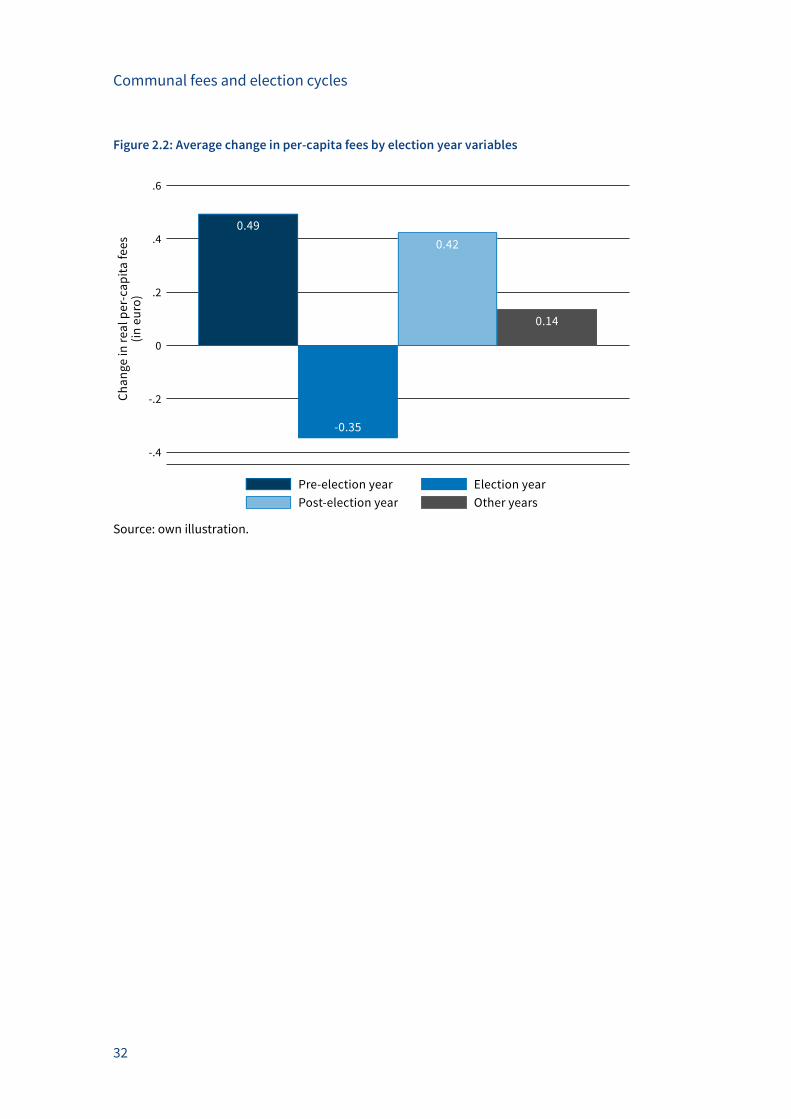
Communal fees and election cycles
32
Figure 2.2: Average change in per-capita fees by election year variables
Source: own illustration.
Communal fees and election cycles
33
Table 2.1: Descriptive statistics
Obs. Mean Std. Dev. Min Max
Fees per capita 108,463 80.78 85.01 0 1,319
∆ Fees per capita 101,199 0.163 20.95 -907.2 458.2
Pre-election year 101,199 0.194 0.395 0 1
Election year 101,199 0.198 0.399 0 1
Post-election year 101,199 0.185 0.388 0 1
Population (t-1) 108,519 8.189 32.52 0.006 1,295
∆ Population (t-1) 86,159 0.017 0.253 -19.89 34.93
Young (t-1) 108,513 0.193 0.035 0.019 0.56
∆ Young (t-1) 86,159 -0.002 0.008 -0.227 0.169
Old (t-1) 108,510 0.182 0.052 0.003 0.536
∆ Old (t-1) 86,159 0.003 0.008 -0.204 0.284
Debt per capita (t-1) 100,725 422.9 405.0 0 12,003
∆ Debt per capita (t-1) 86,159 -0.157 114.7 -2,392 5,771
Property tax B 105,216 304.5 45.17 0 900
∆ Property tax B 86,159 3.265 11.03 -280 280
Business tax 105,216 332.3 30.20 116 900
∆ Business tax 86,159 1.640 7.215 -346 214
Vote share SPD 86,159 0.183 0.190 0 1
Vote share CDU 86,159 0.244 0.232 0 1
Vote share FDP 86,159 0.012 0.032 0 0.578
Vote share Greens 86,159 0.016 0.036 0 0.313
Vote share Others 86,159 0.353 0.360 0 1
Note: Descriptive statistics are calculated for the observations used in the individual regressions. Var-
iables in levels include all observations that are used to calculate the first differences, which are used
in the regressions. I define variables in Section 2.4.2.
Communal fees and election cycles
34
Table 2.2: Correlation between the main variables
∆ Fees per
capita Pre-election year Election year
Post-election
year
∆ Fees per capita 1
Pre-election year 0.008** 1
Election year -0.012*** -0.244*** 1
Post-election year 0.006* -0.234*** -0.237*** 1
Note: * p < 0.10, ** p < 0.05, *** p < 0.01. I define variables in Section 2.4.2.
Table 2.3: Local election dates
State
Baden-Wuerttemberg 12-06-1994 24-10-1999 13-06-2004
Bavaria 10-03-1996 03-03-2002
Hesse 07-03-1993 02-03-1997 18-03-2001 26-03-2006
Lower Saxony 15-09-1996 09-09-2001 10-09-2006
North Rhine-Westphalia 16-10-1994 12-09-1999 26-09-2004
Rhineland-Palatinate 12-06-1994 13-06-1999 13-06-2004
Saarland 12-06-1994 13-06-1999 13-06-2004
Note: Election dates are listed in DD-MM-YYYY.
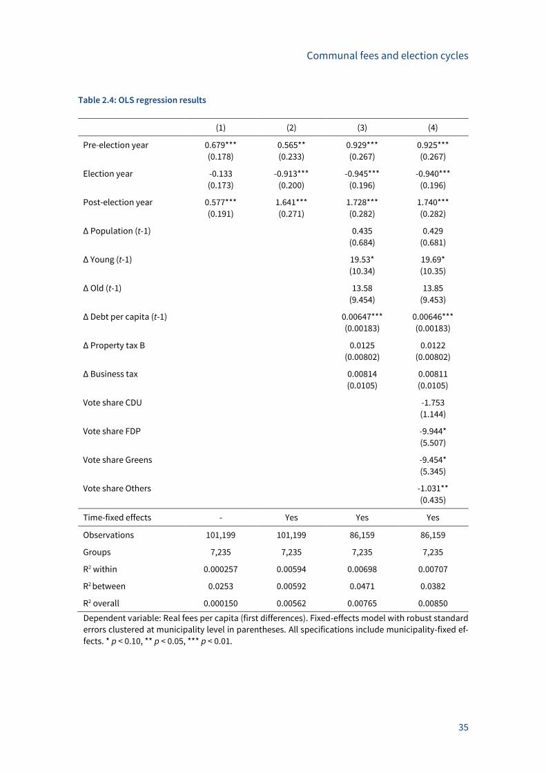
Communal fees and election cycles
35
Table 2.4: OLS regression results
Dependent variable: Real fees per capita (first differences). Fixed-effects model with robust standard
errors clustered at municipality level in parentheses. All specifications include municipality-fixed ef-
fects. * p < 0.10, ** p < 0.05, *** p < 0.01.
(1) (2) (3) (4)
Pre-election year 0.679*** 0.565** 0.929*** 0.925***
(0.178) (0.233) (0.267) (0.267)
Election year -0.133 -0.913*** -0.945*** -0.940***
(0.173) (0.200) (0.196) (0.196)
Post-election year 0.577*** 1.641*** 1.728*** 1.740***
(0.191) (0.271) (0.282) (0.282)
∆ Population (t-1) 0.435 0.429
(0.684) (0.681)
∆ Young (t-1) 19.53* 19.69*
(10.34) (10.35)
∆ Old (t-1) 13.58 13.85
(9.454) (9.453)
∆ Debt per capita (t-1) 0.00647*** 0.00646***
(0.00183) (0.00183)
∆ Property tax B 0.0125 0.0122
(0.00802) (0.00802)
∆ Business tax 0.00814 0.00811
(0.0105) (0.0105)
Vote share CDU -1.753
(1.144)
Vote share FDP -9.944*
(5.507)
Vote share Greens -9.454*
(5.345)
Vote share Others -1.031**
(0.435)
Time-fixed effects - Yes Yes Yes
Observations 101,199 101,199 86,159 86,159
Groups 7,235 7,235 7,235 7,235
R2 within 0.000257 0.00594 0.00698 0.00707
R2 between 0.0253 0.00592 0.0471 0.0382
R2 overall 0.000150 0.00562 0.00765 0.00850
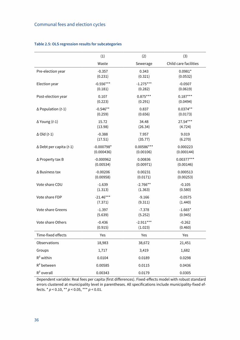
Communal fees and election cycles
36
Table 2.5: OLS regression results for subcategories
(1) (2) (3)
Waste Sewerage Child care facilities
Pre-election year -0.357 0.343 0.0981*
(0.231) (0.321) (0.0532)
Election year -0.556*** -1.275*** -0.0507
(0.181) (0.282) (0.0619)
Post-election year 0.107 0.875*** 0.187***
(0.223) (0.291) (0.0494)
∆ Population (t-1) -0.546** 0.837 0.0374**
(0.259) (0.656) (0.0173)
∆ Young (t-1) 15.72 34.48 27.54***
(13.98) (26.34) (4.724)
∆ Old (t-1) -0.388 7.957 9.019
(17.51) (35.77) (6.270)
∆ Debt per capita (t-1) -0.000798* 0.00586*** 0.000223
(0.000436) (0.00106) (0.000144)
∆ Property tax B -0.000962 0.00836 0.00377***
(0.00534) (0.00971) (0.00146)
∆ Business tax -0.00206 0.00231 0.000513
(0.00958) (0.0171) (0.00253)
Vote share CDU -1.639 -2.766** -0.105
(1.313) (1.363) (0.580)
Vote share FDP -21.46*** -9.166 -0.0575
(7.371) (9.311) (1.440)
Vote share Greens -1.397 -7.378 -1.665*
(5.639) (5.252) (0.945)
Vote share Others -0.436 -2.911*** -0.262
(0.915) (1.023) (0.460)
Time-fixed effects Yes Yes Yes
Observations 18,983 38,672 21,451
Groups 1,717 3,419 1,682
R² within 0.0104 0.0189 0.0298
R² between 0.00585 0.0115 0.0436
R² overall 0.00343 0.0179 0.0305
Dependent variable: Real fees per capita (first differences). Fixed-effects model with robust standard
errors clustered at municipality level in parentheses. All specifications include municipality-fixed ef-
fects. * p < 0.10, ** p < 0.05, *** p < 0.01.
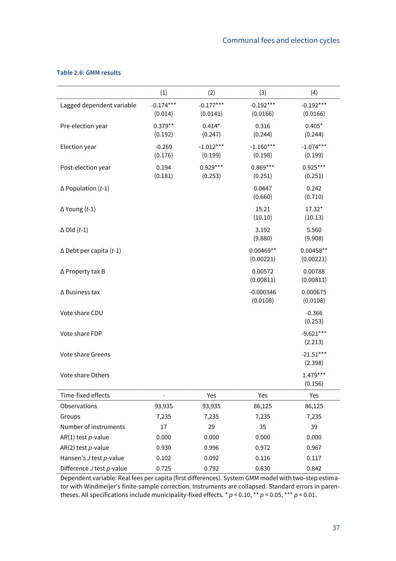
Communal fees and election cycles
37
Table 2.6: GMM results
(1) (2) (3) (4)
Lagged dependent variable -0.174*** -0.177*** -0.192*** -0.192***
(0.014) (0.0141) (0.0166) (0.0166)
Pre-election year 0.379** 0.414* 0.316 0.405*
(0.192) (0.247) (0.244) (0.244)
Election year -0.269 -1.012*** -1.160*** -1.074***
(0.176) (0.199) (0.198) (0.199)
Post-election year 0.194 0.929*** 0.869*** 0.925***
(0.181) (0.253) (0.251) (0.251)
∆ Population (t-1) 0.0447 0.242
(0.660) (0.710)
∆ Young (t-1) 15.21 17.32*
(10.10) (10.13)
∆ Old (t-1) 3.192 5.560
(9.880) (9.908)
∆ Debt per capita (t-1) 0.00469** 0.00458**
(0.00221) (0.00221)
∆ Property tax B 0.00572 0.00788
(0.00811) (0.00811)
∆ Business tax -0.000346 0.000675
(0.0108) (0.0108)
Vote share CDU -0.366
(0.253)
Vote share FDP -9.621***
(2.213)
Vote share Greens -21.51***
(2.398)
Vote share Others 1.479***
(0.156)
Time-fixed effects - Yes Yes Yes
Observations 93,935 93,935 86,125 86,125
Groups 7,235 7,235 7,235 7,235
Number of instruments 17 29 35 39
AR(1) test p-value 0.000 0.000 0.000 0.000
AR(2) test p-value 0.930 0.996 0.972 0.967
Hansen’s J test p-value 0.102 0.092 0.116 0.117
Difference J test p-value 0.725 0.792 0.830 0.842
Dependent variable: Real fees per capita (first differences). System GMM model with two-step estima-
tor with Windmeijer’s finite-sample correction. Instruments are collapsed. Standard errors in paren-
theses. All specifications include municipality-fixed effects. * p < 0.10, ** p < 0.05, *** p < 0.01.

Communal fees and election cycles
38
Electoral cycles in MPs’ salaries
39
3 Electoral cycles in MPs‘ salaries: Evidence from
the German states
Electoral cycles in MPs’ salaries
Abstract*
Members of parliament (MPs) often set their own salaries. Voters dislike self-serving politi-
cians, and politicians are keen to please voters. In line with political business cycle theories,
politicians thus may delay giving themselves a salary increase until after elections. We inves-
tigate electoral cycles in the salary increases of German state MPs. Using data for 15 states
over the period 1980–2014, we find no evidence that increases in MP salaries are influenced
by election cycles. Politicians can increase their salaries at any point during the legislative
period without negative consequences. We posit that this may be because even those voters
who are most disenchanted with politics likely understand that all politicians benefit from a
salary increase and thus do not punish the governing party at the polls.
* This chapter is based on joint work with Björn Kauder and Niklas Potrafke. It is based on our paper “Electoral cycles in MPs’
salaries: Evidence from the German states”, International Tax and Public Finance, 25(4), 981–1000, 2018. We thank Hans Herbert von Arnim, Sutirtha Bagchi, Frank Bohn, Paul Hufe, Stephan Michel, seminar/conference participants at the Public Choice Soci-
ety’s Annual Meeting (Fort Lauderdale 2016), the Spring Meeting of Young Economists (Lisbon 2016), the Meeting of the Associa-
tion for Public Economic Theory (Rio de Janeiro 2016), the Annual Congress of the International Institute of Public Finance (Lake
Tahoe 2016), the Annual Conference of the European Association of Law and Economics (Bologna 2016), the European Public
Choice Society’s Annual Meeting (Budapest 2017), the Annual Conference of the Canadian Economic Association (Antigonish 2017), the University of Munich, and the Ifo Institute, and an anonymous referee for their helpful comments, and Lisa Giani Contini
and Deborah Willow for proofreading. Kristin Fischer, Felix Hugger, Adam Job, Benedikt Kauf, Antonia Kremheller, Sebastian
Kropp, Luisa Lorenz, Julia Richenhagen, Leonard Thielmann, and Johanna Wietschel provided excellent research assistance.
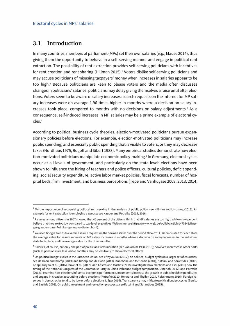
Electoral cycles in MPs’ salaries
40
Introduction
In many countries, members of parliament (MPs) set their own salaries (e.g., Mause 2014), thus
giving them the opportunity to behave in a self-serving manner and engage in political rent
extraction. The possibility of rent extraction provides self-serving politicians with incentives
for rent creation and rent sharing (Hillman 2015).1 Voters dislike self-serving politicians and
may accuse politicians of misusing taxpayers’ money when increases in salaries appear to be
too high.2 Because politicians are keen to please voters and the media often discusses
changes in politicians’ salaries, politicians may delay giving themselves a raise until after elec-
tions. Voters seem to be aware of salary increases: search requests on the internet for MP sal-
ary increases were on average 1.96 times higher in months where a decision on salary in-
creases took place, compared to months with no decisions on salary adjustments.3 As a
consequence, self-induced increases in MP salaries may be a prime example of electoral cy-
cles.4
According to political business cycle theories, election-motivated politicians pursue expan-
sionary policies before elections. For example, election-motivated politicians may increase
public spending, and especially public spending that is visible to voters, or they may decrease
taxes (Nordhaus 1975, Rogoff and Sibert 1988). Many empirical studies demonstrate how elec-
tion-motivated politicians manipulate economic policy-making.5 In Germany, electoral cycles
occur at all levels of government, and particularly on the state level: elections have been
shown to influence the hiring of teachers and police officers, cultural policies, deficit spend-
ing, social security expenditure, active labor market policies, fiscal forecasts, number of hos-
pital beds, firm investment, and business perceptions (Tepe and Vanhuysse 2009, 2013, 2014,
1 On the importance of recognizing political rent seeking in the analysis of public policy, see Hillman and Ursprung (2016). An
example for rent extraction is employing a spouse; see Kauder and Potrafke (2015, 2016).
2 A survey among citizens in 2007 showed that 46 percent of the citizens think that MP salaries are too high, while only 4 percent
believe that they are too low compared to top-level executives (Welt online, see https://www. welt.de/politik/article1475841/Buer-
ger-glauben-dass-Politiker-genug-verdienen.html).
3 We used Google Trends to examine search requests in the German states over the period 2004–2014. We calculated for each state
the average value for search requests on MP salary increases in months where a decision on salary increases in the individual
state took place, and the average value for the other months.
4 Salaries, of course, are only one part of politicians’ remuneration (see von Arnim 1998, 2010); however, increases in other parts
(such as pensions) are less visible and thus may be less likely to show electoral effects.
5 On political budget cycles in the European Union, see Efthyvoulou (2012); on political budget cycles in a larger set of countries,
see de Haan and Klomp (2013) and Klomp and de Haan (2013). Kneebone and McKenzie (2001), Katsimi and Sarantides (2012),
Köppl-Turyna et al. (2016), Bove et al. (2017), and Castro and Martins (2018) investigate how elections and Tsai (2016) how the
timing of the National Congress of the Communist Party in China influence budget composition. Osterloh (2012) and Potrafke (2012a) examine how elections influence economic performance. Incumbents increase the growth in public health expenditures
and engage in creative accounting before elections (Potrafke 2010, Herwartz and Theilen 2014, Reischmann 2016). Foreign re-
serves in democracies tend to be lower before elections (Jäger 2016). Transparency may mitigate political budget cycles (Benito
and Bastida 2009). On public investment and reelection prospects, see Katsimi and Sarantides (2015).
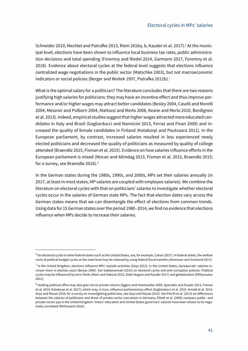
Electoral cycles in MPs’ salaries
41
Schneider 2010, Mechtel and Potrafke 2013, Riem 2016a, b, Kauder et al. 2017).6 At the munic-
ipal level, elections have been shown to influence local business tax rates, public administra-
tion decisions and total spending (Foremny and Riedel 2014, Garmann 2017, Foremny et al.
2018). Evidence about electoral cycles at the federal level suggests that elections influence
centralized wage negotiations in the public sector (Matschke 2003), but not macroeconomic
indicators or social policies (Berger and Woitek 1997, Potrafke 2012b).7
What is the optimal salary for a politician? The literature concludes that there are two reasons
justifying high salaries for politicians: they may have an incentive effect and thus improve per-
formance and/or higher wages may attract better candidates (Besley 2004, Caselli and Morelli
2004, Messner and Polborn 2004, Mattozzi and Merlo 2008, Keane and Merlo 2010, Bordignon
et al. 2013). Indeed, empirical studies suggest that higher wages attracted more educated can-
didates in Italy and Brazil (Gagliarducci and Nannicini 2013, Ferraz and Finan 2009) and in-
creased the quality of female candidates in Finland (Kotakorpi and Poutvaara 2011). In the
European parliament, by contrast, increased salaries resulted in less experienced newly
elected politicians and decreased the quality of politicians as measured by quality of college
attended (Braendle 2015, Fisman et al. 2015). Evidence on how salaries influence efforts in the
European parliament is mixed (Mocan and Altindag 2013, Fisman et al. 2015, Braendle 2015;
for a survey, see Braendle 2016).8
In the German states during the 1980s, 1990s, and 2000s, MPs set their salaries annually (in
2017, at least in most states, MP salaries are coupled with employee salaries). We combine the
literature on electoral cycles with that on politicians’ salaries to investigate whether electoral
cycles occur in the salaries of German state MPs. The fact that election dates vary across the
German states means that we can disentangle the effect of elections from common trends.
Using data for 15 German states over the period 1980–2014, we find no evidence that elections
influence when MPs decide to increase their salaries.
6 On electoral cycles in other federal states such as the United States, see, for example, Cahan (2017). In federal states, the welfare
costs of political budget cycles at the state level may be reduced by using federal fiscal transfers (Aronsson and Granlund 2017).
7 In the United Kingdom, elections influence MPs’ outside activities (Geys 2013). In the United States, bureaucrats’ salaries in-
crease more in election years (Borjas 1984). See Vadlamannati (2015) on electoral cycles and anti-corruption policies. Political cycles may be influenced by term limits (Klein and Sakurai 2015, Dalle Nogare and Kauder 2017) and globalization (Efthyvoulou
2011).
8 Holding political office may also give rise to private returns (Eggers and Hainmueller 2009, Querubin and Snyder 2013, Fisman
et al. 2014, Kotakorpi et al. 2017), which may, in turn, influence parliamentary effort (Gagliarducci et al. 2010, Arnold et al. 2014, Geys and Mause 2016; for a survey on moonlighting politicians, see Geys and Mause 2013). See Peichl et al. (2013) on differences
between the salaries of politicians and those of private-sector executives in Germany; Elliott et al. (2005) compare public- and
private-sector pay in the United Kingdom. Voters’ education and United States governors’ salaries have been shown to be nega-
tively correlated (Mirhosseini 2016).
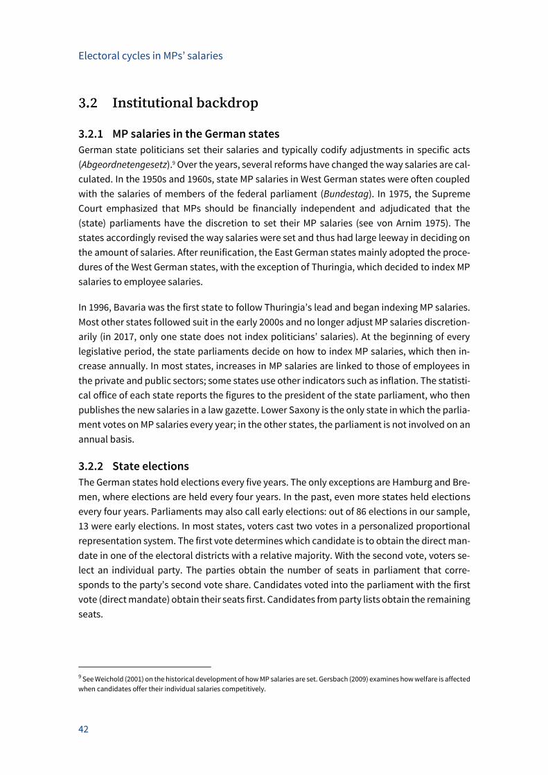
Electoral cycles in MPs’ salaries
42
Institutional backdrop
3.2.1 MP salaries in the German states
German state politicians set their salaries and typically codify adjustments in specific acts
(Abgeordnetengesetz).9 Over the years, several reforms have changed the way salaries are cal-
culated. In the 1950s and 1960s, state MP salaries in West German states were often coupled
with the salaries of members of the federal parliament (Bundestag). In 1975, the Supreme
Court emphasized that MPs should be financially independent and adjudicated that the
(state) parliaments have the discretion to set their MP salaries (see von Arnim 1975). The
states accordingly revised the way salaries were set and thus had large leeway in deciding on
the amount of salaries. After reunification, the East German states mainly adopted the proce-
dures of the West German states, with the exception of Thuringia, which decided to index MP
salaries to employee salaries.
In 1996, Bavaria was the first state to follow Thuringia’s lead and began indexing MP salaries.
Most other states followed suit in the early 2000s and no longer adjust MP salaries discretion-
arily (in 2017, only one state does not index politicians’ salaries). At the beginning of every
legislative period, the state parliaments decide on how to index MP salaries, which then in-
crease annually. In most states, increases in MP salaries are linked to those of employees in
the private and public sectors; some states use other indicators such as inflation. The statisti-
cal office of each state reports the figures to the president of the state parliament, who then
publishes the new salaries in a law gazette. Lower Saxony is the only state in which the parlia-
ment votes on MP salaries every year; in the other states, the parliament is not involved on an
annual basis.
3.2.2 State elections
The German states hold elections every five years. The only exceptions are Hamburg and Bre-
men, where elections are held every four years. In the past, even more states held elections
every four years. Parliaments may also call early elections: out of 86 elections in our sample,
13 were early elections. In most states, voters cast two votes in a personalized proportional
representation system. The first vote determines which candidate is to obtain the direct man-
date in one of the electoral districts with a relative majority. With the second vote, voters se-
lect an individual party. The parties obtain the number of seats in parliament that corre-
sponds to the party’s second vote share. Candidates voted into the parliament with the first
vote (direct mandate) obtain their seats first. Candidates from party lists obtain the remaining
seats.
9 See Weichold (2001) on the historical development of how MP salaries are set. Gersbach (2009) examines how welfare is affected
when candidates offer their individual salaries competitively.
Electoral cycles in MPs’ salaries
43
Empirical analysis
3.3.1 Descriptive statistics
We use data on MPs’ nominal salaries taken from state law gazettes, as well as data from the
federal and the states’ statistical offices, the state election administrators, the German Bun-
destag, and the German Council of Economic Experts. We use annual data over the period
1980–2014 for the West German states and over the period 1991–2014 for the East German
states. We only use data for non-indexed years, meaning that for some states, our data end
earlier than 2014 because these states began indexing MP salaries prior to that year (see Sec-
tion 3.2.1). We exclude Thuringia because MP salaries in Thuringia are coupled with the gen-
eral development of wages since 1990. We also exclude increases in salaries of over 20 per-
cent, which represent increases after reforms in parliament such as adjusting the taxation of
salaries or when parliaments declared to transform a part-time parliament into a full-time
parliament.10 The sample includes 15 states and 367 observations.11
Figure 3.1 shows the average increase in MPs’ nominal salaries after and before elections. MP
salaries increased on average by 1.99 percent when it was the first increase within the 365
days after an election, and by 2.07 percent when it was the last increase within the 365 days
before an election. At other times during the legislative period, MP salaries increased on aver-
age by 2.53 percent. T-tests on means indicate that neither post-election nor pre-election in-
creases are significantly different from increases at other points in time.
To more clearly see the nexus between points of time in a legislative period and increases in
salaries, the left part of Figure 3.2 shows the result of a nonparametric regression of increases
in salaries on the share of a legislative period that has passed, using kernel-weighted local
polynomial smoothing; the right part shows a semi-parametric regression including all our
(parametric) control variables (see Boone et al. 2014, pp. 404–407). Both panels corroborate
the evidence from Figure 3.1 and suggest that MP salaries increased somewhat less at the be-
ginning and at the end of a legislative period. The regular pattern of local minima arises from
our coding of pay freezes (see footnote 11).
Table 3.1 sets out descriptive statistics. Table 3.2 contains the correlation coefficients be-
tween our main variables. Increases in MP salaries are barely correlated with the post-election
10 There were 14 salary increases above 20 percent during 1980–2014. In a part-time parliament, politicians may well work in
addition to their parliamentary function. In a full-time parliament, the parliamentary function is full-time and other professional
activities are possible only to a limited extent.
11 In some cases, salaries were not increased. To define the dates on which these pay freezes were decided on, we use the average
day on which increases in salaries were decided on in other years in the respective state. In our sample, we defined 172 artificial
dates for the pay freezes.
Electoral cycles in MPs’ salaries
44
and pre-election dummy variables (correlation coefficients: -0.05 and -0.04) or with the num-
ber of days since the last election (0.02). Increases in MP salaries and in lagged employee sal-
aries are somewhat correlated (0.34); see also Figure 3.3.
3.3.2 Empirical strategy
The baseline panel-data model has the following form:
Increase in MP salariesi,t = β Post-election periodi,t + γ Pre-election periodi,t
+ δ Increase in employee salariesi,t-1 + ε Deficit ratioi,t-1
+ ζ Government ideologyi,t + φ Seat share governmenti,t + ηi + τt + ui,t
with i = 1,…,15; t = 1,…,35
where Increase in MP salariesi,t measures the increase in MPs’ nominal salaries in state i in year
t (growth rate). The dummy variable Post-election periodi,t assumes the value of 1 for the first
increase in salaries within the 365 days after an election and is 0 otherwise. The dummy vari-
able Pre-election periodi,t takes the value of 1 for the last increase in salaries within the 365
days before an election.12 The reference category is thus the period between the post- and the
pre-election period (note that predetermined elections are not prone to reverse causality). In
alternative specifications, we use a variable measuring the number of days since the last elec-
tion divided by the total length of the legislative period (Share of legislative period passedi,t)
instead of dummy variables for the post- and the pre-election periods.13 Concerns about po-
tential endogeneity of the election variables include reverse causality and omitted variable
bias. The election variables are not prone to reverse causality because we deal with early elec-
tions. To limit the risk of omitted variable bias, we include many variables that are likely to be
correlated with an increase in MP salaries and/or the election variables.
Increase in employee salariesi,t-1 measures the extent to which salaries of public- and private-
sector employees increased in the previous year (see also Di Tella and Fisman 2004); we con-
sider nominal values of salaries and thus capture both increases in real salaries and inflation.
We expect the salaries of private- and public-sector employees to be positively correlated with
MP salaries. The variable Deficit ratioi,t-1 measures how public debt has increased relative to
GDP in state i in year t-1 and is expected to be negatively correlated with MP salaries, under
the assumption that MPs are unlikely to increase their salaries when public debt has increased
and the topic of how to decrease the debt is a matter of public debate. The variable Govern-
ment ideologyi,t measures ideology-induced policy-making and takes the value of 1 when a
12 Note that we only consider the salary increases closest to the election when there was more than one increase in the 365 days
after or before an election. In the case of early elections, we consider an increase in salaries only as belonging to the pre-election
period when early elections were known at that point of time.
13 In the case of early elections, we consider the regular length of a legislative period when salaries were increased before early
elections were called, and the actual length when salaries were increased after early elections were called.
Electoral cycles in MPs’ salaries
45
left-wing government is in office, the value 0.5 for a center government, and is 0 for a right-
wing government (e.g., Kauder and Potrafke 2013, Potrafke et al. 2016). The extent to which
government ideology correlates with MP salaries is not clear. On the one hand, right-wing gov-
ernments may believe that MP salaries should be competitive with those of managers or en-
trepreneurs. On the other hand, right-wing governments favor a smaller size of government
than do left-wing governments, and thus, when they are in power, MP salaries may be less
generous. It is conceivable that politicians set higher salaries for themselves when their party
holds a large majority of seats in parliament (see Benito et al. 2014, Svaleryd and Vlachos
2009). Seat share governmenti,t thus measures the number of seats of the governing parties
relative to all seats in parliament. ηi is a fixed state effect; τt is a fixed time effect; ui,t is the error
term. In some specifications, we include the variable Increase in federal MP (nominal) salariesi,t-
1, which varies only over time and not over states, instead of fixed time effects. We estimate
the fixed effects model with standard errors robust to heteroskedasticity (Huber/White/sand-
wich standard errors; see Huber 1967, White 1980).
3.3.3 Regression results
Table 3.3 shows the regression results excluding fixed time effects. In discussing the results,
we focus on our preferred specification (Column 3), which includes all control variables. The
coefficients of the dummy variables Post-election period and Pre-election period are negative
and thus corroborate the graphical evidence, but lack statistical significance. Increases in MP
salaries are positively correlated with increases in employee salaries. The effect attains statis-
tical significance at the 1 percent level and indicates that MP salaries respond with an increase
of 0.30 percent to a 1 percent increase in employee salaries in the previous year. The effect is
small, but the constant shows a significant effect, indicating that MP salaries increased by 2.65
percent per year (conditional on the other explanatory variables) and politicians thus smooth
salary increases over time. Our other control variables (lagged) Deficit ratio, Government ide-
ology, and (lagged) Increase in federal MP salaries do not turn out to be statistically significant.
The effect of the variable Seat share government indicates that powerful governments in-
crease MP salaries relatively less; however, the effect is statistically significant only at the 10
percent level.
In Table 3.4, we include fixed time effects and thus cannot include Increase in federal MP sala-
ries because this variable does not vary across states. Inferences regarding the election period
dummies and the effect of employee salaries do not change. However, Seat share government
loses statistical significance when we include fixed time effects.
Table 3.5 shows the results (excluding fixed time effects) when we use the Share of legislative
period passed (share of legislative period that has passed at the time MPs decide to increase
their salaries) as the main explanatory variable; the effect lacks, however, statistical signifi-
cance. The coefficient estimate of Increase in employee salaries corroborates our results from
Table 3.3 and Table 3.4 and indicates that increases in MP and (lagged) employee salaries are
Electoral cycles in MPs’ salaries
46
positively correlated. Inferences do not change when we include a quadratic term of Share of
legislative period passed (Columns 4–6): the specifications indicate an inverted u-shaped rela-
tionship between the share of a legislative period that has passed and increases in MP salaries
and thus corroborate the graphical evidence from Figure 3.2. Again, however, the effects fail
to reach statistical significance at conventional levels. The effects of Share of legislative period
passed and its quadratic term also lack statistical significance when we include fixed time ef-
fects in Table 3.6.14
As a placebo test, we include in Table 3.7 the indexed years in our sample, increasing sample
size to 478 observations. Inferences regarding the election period dummies and the effect of
the continuous time variable Share of legislative period passed do not change regardless of
whether fixed time effects are included or excluded. This also holds for employee salaries.
In Table 3.8, we run the regressions for the indexed years only (111 observations). The coeffi-
cients of the election period dummies and employee salaries lack statistical significance. The
effect of Share of legislative period passed and its quadratic term also lack statistical signifi-
cance. The variable Government ideology is statistically significant in only one specification.
3.3.4 Robustness tests
We submitted our results to rigorous robustness tests using different specifications of our
regressions and different samples. None of these robustness tests indicates any severe
fragility in our results.
We estimated our baseline panel-data model with a fixed effects estimator. However, because
many observations of salary increases are zero, a Tobit model may be more suitable. When
we use a Tobit cross-section estimator (a parametric conditional fixed effects Tobit panel
estimator is not available), the results indicate that MPs increase their salaries less after
elections and, in some specifications, also less before elections. The effect of the continuous
time variable Share of legislative period passed is statistically significant when we also include
its quadratic term. The coefficients of both variables indicate that politicians increase their
salaries in the middle of the legislative period, thus corroborating the graphical evidence from
Figure 3.2. Inferences compared to our baseline model do not change when we use a random
effects model. Inferences with a random effects Tobit model are similar to those with a Tobit
cross-section estimator.
As an alternative to considering the growth rate of MP salaries as the dependent variable, we
used a binary variable that takes the value 1 when salaries were increased and 0 otherwise.
With either a probit or logit model, the results show that the probability of an increase in
salaries was lower after and before elections. Given the results in Table 3.3 and Table 3.4, this
14 By excluding fixed state effects, the continuous time variable is positive and statistically significant at the 10 percent level.
Electoral cycles in MPs’ salaries
47
indicates that positive increases in MP salaries were higher after and before elections. In fact,
if increases were positive, they were on average 4.69 percent after an election and 4.96
percent before an election, but only 4.31 percent at other times.15 The effect of the continuous
time variable Share of legislative period passed is statistically significant when we also include
its quadratic term.
We also investigated whether it was only extraordinary increases in salaries that were
influenced by electoral cycles. To this end, we used a binary variable as the dependent
variable that takes the value 1 when MP salaries increased more than (lagged) employee
salaries. Again, the results from either a probit or logit model show that the probability of MP
salaries increasing more than those of employees was lower before and after elections. We
tested whether inferences change when we included the lagged level of MP salaries to control
for mean reversion. The results show that a higher lagged level of MP salaries decreased the
growth rate of salaries when fixed time effects are excluded, but still do not show that
elections influenced salary increases.
In constructing our main explanatory variables Post-election period and Pre-election period,
we captured increases in salaries within the 365 days after or before an election. Inferences
do not change when we capture salary increases within 0.5 years or 1.5 years after or before
an election. Our alternative main explanatory variable Share of legislative period passed is
defined as the number of days since the last election divided by the total length of the
legislative period. Inferences do not change when we use the number of days since the last
election (without dividing by the length of the legislative period) as an explanatory variable.
We investigated the possibility of electoral cycles in MP salary increases in combination with
changes of government. We revised our two dummy variables in the way that both variables
assume the value 1 for the first (last) increase in salaries within the 365 days after (before) an
election only if a change of government happened at that election. Inferences regarding
electoral cycles do not change when we revise our dummy variables.
We tested whether inferences change when we include Increase in employee salaries, Deficit
ratio, and Increase in federal MP salaries from the respective year and not in lags. The results
show that Increase in employee salaries does not turn out to be statistically significant when
we include fixed time effects, but remains statistically significant when we exclude fixed time
effects. The coefficient of Deficit ratio is positive and statistically significant in all
specifications. The effect of Increase in federal MP salaries is statistically significant only in
some specifications. The election period dummy variables do not turn out to be statistically
significant in any of the specifications. The coefficient of the continuous time variable Share
of legislative period passed is statistically significant only when we include its quadratic term
15 A t-test on means shows that neither post-election nor pre-election increases are significantly different from positive increases
at other times.
Electoral cycles in MPs’ salaries
48
and when we exclude fixed time effects. We also tested whether inferences change when we
use Increase in employee salaries and Increase in federal MP salaries in real terms and include
lagged inflation as another control variable to disentangle the effects of real salaries’
increases and inflation. Inferences do not change.
Our measure of employee salaries includes net salaries, income tax, and employees’ social
security contributions. Inferences regarding electoral cycles and the effect of increases in
employee salaries do not change when we use an alternative measure of employee salaries
that also includes employers’ social security contributions. Neither do inferences regarding
electoral cycles change when we replace the (lagged) growth in employee salaries with the
(lagged) growth in GDP, which is statistically significant at the 10 percent level only in some
specifications. To describe the power of a government, we used the seat share of the
governing parties in parliament. Inferences regarding electoral cycles and the effect of the
power of a government do not change when we use the vote share of the governing parties
divided by the vote share of all parties represented in parliament.
We examined whether our results are driven by individual years or individual states. When we
exclude individual years or states, one at a time (jackknife test), the results still do not show
electoral cycles in MP salaries when we use the electoral period dummies or the share of the
legislative period that has passed as main explanatory variables. When we include the
quadratic term of Share of legislative period passed, the results indicate that MP salaries
increased less after and before elections when we exclude the years 1985 or 1993, or the state
Baden-Wuerttemberg.
Politicians in the East German states may well differ from politicians in the West German
states. The results of separate regressions for East German and West German states do not
reveal electoral cycles in MP salaries.
It is conceivable that electoral cycles occur only under some type of government ideology. We
thus estimated our model separately for left-wing, right-wing, and center governments. The
results do not show electoral cycles in MP decisions on increases in salaries.
Conclusion
During the 1980s, 1990s, and 2000s, German state MPs annually set their own salaries, making
German states an excellent laboratory for electoral manipulation. We investigated whether
elections influence increases in MP salaries. The results do not show (robust) evidence for
electoral cycles in decisions about increasing MP salaries, nor do government ideology or the
power of the government influence MP salaries. We do find, however, that increases in MP
salaries are positively correlated with increases in employee salaries.
Electoral cycles in MPs’ salaries
49
Why is it that increases in MP salaries do not exhibit an electoral cycle? When MPs increase
their salaries, they do so for all MPs, not only for government MPs. Certainly, voters may pun-
ish government politicians for having initiated and voted for salary increases. However, we
conjecture that even those voters who are most disenchanted with politics likely understand
that all politicians benefit from a salary increase, and thus, there may be no party-specific
election ramifications. In short, politicians can give themselves a raise at any point of time
without having to fear negative voter reaction. This also explains why governments with a
large majority in parliament do not increase salaries more than governments with a fragile
majority.
Electoral cycles in MPs’ salaries
50
References
Arnold, F., B. Kauder, and N. Potrafke (2014). Outside earnings, absence, and activity: Evidence
from German parliamentarians. European Journal of Political Economy, 36, 147–157.
Aronsson, T. and D. Granlund (2017). Federal subsidization of state expenditure to reduce po-
litical budget cycles. International Tax and Public Finance, 24, 536–545.
Benito, B. and F. Bastida (2009). Budget transparency, fiscal performance, and political turn-
out: An international approach. Public Administration Review, 69, 403–417.
Benito, B., F. Bastida, A.-M. Ríos, and C. Vicente (2014). The causes of legal rents extraction:
Evidence from Spanish municipalities. Public Choice, 161, 367–383.
Berger, H. and U. Woitek (1997). Searching for political business cycles in Germany. Public
Choice, 91, 179–197.
Besley, T. (2004). Paying politicians: Theory and evidence. Journal of the European Economic
Association, 2, 193–215.
Boone, C., A. Dube, and E. Kaplan (2014). The political economy of discretionary spending:
Evidence from the American Recovery and Reinvestment Act. Brookings Papers on Eco-
nomic Activity, Spring, 375–441.
Bordignon, M., M. Gamalerio, and G. Turati (2013). Decentralization, vertical fiscal imbalance,
and political selection. CESifo Working Paper 4459.
Borjas, G. (1984). Electoral cycles and the earnings of federal bureaucrats. Economic Inquiry,
22, 447–459.
Bove, V., G. Efthyvoulou, and A. Navas (2017). Political cycles in public expenditure: Butter ver-
sus guns. Journal of Comparative Economics, 45, 582–604.
Braendle, T. (2015). Does remuneration affect the discipline and the selection of politicians?
Evidence from pay harmonization in the European Parliament. Public Choice, 162, 1–24.
Braendle, T. (2016). Do institutions affect citizens’ selection into politics? Journal of Economic
Surveys, 30, 205–227.
Cahan, D. (2017). Electoral cycles in government employment: Evidence from US gubernato-
rial elections. UCSD Working Paper.
Caselli, F. and M. Morelli (2004). Bad politicians. Journal of Public Economics, 88, 759–782.
Castro, V. and R. Martins (2018). Politically driven cycles in fiscal policy: In depth analysis of
the functional components of government expenditures. European Journal of Political
Economy, forthcoming.
Dalle Nogare, C. and B. Kauder (2017). Term limits for mayors and intergovernmental grants:
Evidence from Italian cities. Regional Science and Urban Economics, 64, 1–11.
Electoral cycles in MPs’ salaries
51
De Haan, J. and J. Klomp (2013). Conditional political budget cycles: A review of recent evi-
dence. Public Choice, 157, 387–410.
Di Tella, R. and R. Fisman (2004). Are politicians really paid like bureaucrats? Journal of Law
and Economics, 47, 477–513.
Efthyvoulou, G. (2011). Political cycles under external economic constraints: Evidence from
Cyprus. Journal of Economics and Business, 63, 638–662.
Efthyvoulou, G. (2012). Political budget cycles in the European Union and the impact of polit-
ical pressures. Public Choice, 153, 295–327.
Eggers, A. C. and J. Hainmueller (2009). MPs for sale? Returns to office in postwar British poli-
tics. American Political Science Review, 103, 513–533.
Elliott, R. F., D. Bell, A. Scott, A. Ma, and E. Roberts (2005). Devolved government and public
sector pay reform: Considerations of equity and efficiency. Regional Studies, 39, 519–
539.
Ferraz, C. and F. Finan (2009). Motivating politicians: The impacts of monetary incentives on
quality and performance. NBER Working Paper 14906.
Fisman, R., N. Harmon, E. Kamenica, and I. Munk (2015). Labor supply of politicians. Journal
of the European Economic Association, 13, 871–905.
Fisman, R., F. Schulz, and V. Vig (2014). The private returns to public office. Journal of Political
Economy, 122, 806–862.
Foremny, D., R. Freier, M.-D. Moessinger, and M. Yeter (2018). Overlapping political budget cy-
cles. Public Choice, 177, 1–27.
Foremny, D. and N. Riedel (2014). Business taxes and the electoral cycle. Journal of Public Eco-
nomics, 115, 48–61.
Gagliarducci, S. and T. Nannicini (2013). Do better paid politicians perform better? Disentan-
gling incentives from selection. Journal of the European Economic Association, 11, 369–
398.
Gagliarducci, S., T. Nannicini, and P. Naticchioni (2010). Moonlighting politicians. Journal of
Public Economics, 94, 688–699.
Garmann, S. (2017). Electoral cycles in public administration decisions: Evidence from Ger-
man municipalities. Regional Studies, 51, 712–723.
Gersbach, H. (2009). Competition of politicians for wages and office. Social Choice and Welfare,
33, 51–71.
Geys, B. (2013). Election cycles in MPs’ outside interests? The UK House of Commons, 2005–
2010. Political Studies, 61, 462–472.
Electoral cycles in MPs’ salaries
52
Geys, B. and K. Mause (2013). Moonlighting politicians: A survey and research agenda. Journal
of Legislative Studies, 19, 76–97.
Geys, B. and K. Mause (2016). The limits of electoral control: Evidence from last-term politi-
cians. Legislative Studies Quarterly, 41, 873–898.
Herwartz, H. and B. Theilen (2014). Health care and ideology: A reconsideration of political
determinants of public healthcare funding in the OECD. Health Economics, 23, 225–240.
Hillman, A. L. (2015). Rent seeking as political economy. In: R. D. Congleton and A. L. Hillman
(Eds.), Companion to the Political Economy of Rent Seeking. Cheltenham: Edward Elgar,
pp. 10–16.
Hillman, A. L. and H. W. Ursprung (2016). Where are the rent seekers? Constitutional Political
Economy, 27, 124–141.
Huber, P. J. (1967). The behavior of maximum likelihood estimates under nonstandard condi-
tions. In: Proceedings of the Fifth Berkeley Symposium on Mathematical Statistics and
Probability, pp. 221–233.
Jäger, K. (2016). The role of regime type in the political economy of foreign reserve accumula-
tion. European Journal of Political Economy, 44, 79–96.
Katsimi, M. and V. Sarantides (2012). Do elections affect the composition of fiscal policy in de-
veloped, established democracies? Public Choice, 151, 325–362.
Katsimi, M. and V. Sarantides (2015). Public investment and reelection prospects in developed
countries. Southern Economic Journal, 82, 471–500.
Kauder, B. and N. Potrafke (2013). Government ideology and tuition fee policy: Evidence from
the German states. CESifo Economic Studies, 59, 628–649.
Kauder, B. and N. Potrafke (2015). Just hire your spouse! Evidence from a political scandal in
Bavaria. European Journal of Political Economy, 38, 42–54.
Kauder, B. and N. Potrafke (2016). Supermajorities and political rent extraction. Kyklos, 68, 65–
81.
Kauder, B., N. Potrafke, and C. Schinke (2017). Manipulating fiscal forecasts: Evidence from
the German states. FinanzArchiv/Public Finance Analysis, 73, 213–236.
Keane, M. P. and A. Merlo (2010). Money, political ambition, and the career decisions of politi-
cians. American Economic Journal: Microeconomics, 2, 186–215.
Klein, F. A. and S. N. Sakurai (2015). Term limits and political budget cycles at the local level:
Evidence from a young democracy. European Journal of Political Economy, 37, 21–36.
Klomp, J. and J. de Haan (2013). Political budget cycles and election outcomes. Public Choice,
157, 245–267.
Electoral cycles in MPs’ salaries
53
Kneebone, R. D. and K. J. McKenzie (2001). Electoral and partisan cycles in fiscal policy: An
examination of Canadian provinces. International Tax and Public Finance, 8, 753–774.
Köppl-Turyna, M., G. Kula, A. Balmas, and K. Waclawska (2016). The effects of fiscal decentral-
ization on the strength of political budget cycles in local expenditure. Local Government
Studies, 42, 785–820.
Kotakorpi, K. and P. Poutvaara (2011). Pay for politicians and candidate selection: An empiri-
cal analysis. Journal of Public Economics, 95, 877–885.
Kotakorpi, K., P. Poutvaara, and M. Terviö (2017). Returns to office in national and local poli-
tics: A bootstrap method and evidence from Finland. Journal of Law, Economics, and
Organization, 33, 413–442.
Matschke, X. (2003). Are there election cycles in wage agreements? An analysis of German pub-
lic employees. Public Choice, 114, 103–135.
Mattozzi, A. and A. Merlo (2008). Political careers or career politicians? Journal of Public Eco-
nomics, 92, 597–608.
Mause, K. (2014). Self-serving legislators? An analysis of the salary-setting institutions of 27 EU
parliaments. Constitutional Political Economy, 25, 154–176.
Mechtel, M. and N. Potrafke (2013). Electoral cycles in active labor market policies. Public
Choice, 156, 181–194.
Messner, M. and M. K. Polborn (2004). Paying politicians. Journal of Public Economics, 88, 2423–
2445.
Mirhosseini, M. R. (2016). Optimal wages for politicians. Southern Economic Journal, 82, 1004–
1020.
Mocan, N. and D. T. Altindag (2013). Salaries and work effort: An analysis of the European Un-
ion parliamentarians. Economic Journal, 123, 1130–1167.
Nordhaus, W. D. (1975). The political business cycle. Review of Economic Studies, 42, 169–190.
Osterloh, S. (2012). Words speak louder than actions: The impact of politics on economic per-
formance. Journal of Comparative Economics, 40, 318–336.
Peichl, A., N. Pestel, and S. Siegloch (2013). The politicians’ wage gap: Insights from German
members of parliament. Public Choice, 156, 653–676.
Potrafke, N. (2010). The growth of public health expenditures in OECD countries: Do govern-
ment ideology and electoral motives matter? Journal of Health Economics, 29, 797–810.
Potrafke, N. (2012a). Political cycles and economic performance in OECD countries: Empirical
evidence from 1951–2006. Public Choice, 150, 155–179.
Potrafke, N. (2012b). Is German domestic social policy politically controversial? Public Choice,
153, 393–418.
Electoral cycles in MPs’ salaries
54
Potrafke, N., M. Riem, and C. Schinke (2016). Debt brakes in the German states: Governments’
rhetoric and actions. German Economic Review, 17, 253–275.
Querubin, P. and J. M. Snyder Jr. (2013). The control of politicians in normal times and times
of crisis: Wealth accumulation by U.S. congressmen, 1850–1880. Quarterly Journal of
Political Science, 8, 409–450.
Reischmann, M. (2016). Creative accounting and electoral motives: Evidence from OECD coun-
tries. Journal of Comparative Economics, 44, 243–257.
Riem, M. (2016a). Corporate investment decisions under political uncertainty. Ifo Working Pa-
per 221.
Riem, M. (2016b). Does political uncertainty influence firm owners’ business perceptions? Ifo
Working Paper 226.
Rogoff, K. and A. Sibert (1988). Elections and macroeconomic policy cycles. Review of Eco-
nomic Studies, 55, 1–16.
Schneider, C. (2010). Fighting with one hand tied behind the back: Political budget cycles in
the West German states. Public Choice, 142, 125–150.
Svaleryd, H. and J. Vlachos (2009). Political rents in a non-corrupt democracy. Journal of Pub-
lic Economics, 93, 355–372.
Tepe, M. and P. Vanhuysse (2009). Educational business cycles. Public Choice, 139, 61–82.
Tepe, M. and P. Vanhuysse (2013). Cops for hire? The political economy of police employment
in the German states. Journal of Public Policy, 33, 165–199.
Tepe, M. and P. Vanhuysse (2014). A vote at the opera? The political economy of public thea-
ters and orchestras in the German states. European Journal of Political Economy, 36,
254–273.
Tsai, P.-H. (2016). Fiscal incentives and political budget cycles in China. International Tax and
Public Finance, 23, 1030–1073.
Vadlamannati, K. C. (2015). Fighting corruption or elections? The politics of anti-corruption
policies in India: A subnational study. Journal of Comparative Economics, 43, 1035–1052.
von Arnim, H. H. (1975). Abgeordnetenentschädigung und Grundgesetz. Wiesbaden: Karl-
Bräuer-Institut des Bundes der Steuerzahler.
von Arnim, H. H. (1998). Diener vieler Herren – Die Doppel- und Dreifachversorgung von Politi-
kern. München: Knaur.
von Arnim, H. H. (2010). Die Privilegien von Landespolitikern. Zeitschrift für Rechtspolitik, 43,
56–57.
Electoral cycles in MPs’ salaries
55
Weichold, J. (2001). Der Abgeordnete und die Diäten. Zum verfassungsrechtlichen Problem
der “angemessenen”, die “Unabhängigkeit” des Abgeordneten sichernden Entschädi-
gung. UTOPIE kreativ, 125, 232–241.
White, H. (1980). A heteroskedasticity-consistent covariance matrix estimator and a direct test
for heteroskedasticity. Econometrica, 48, 817–838.
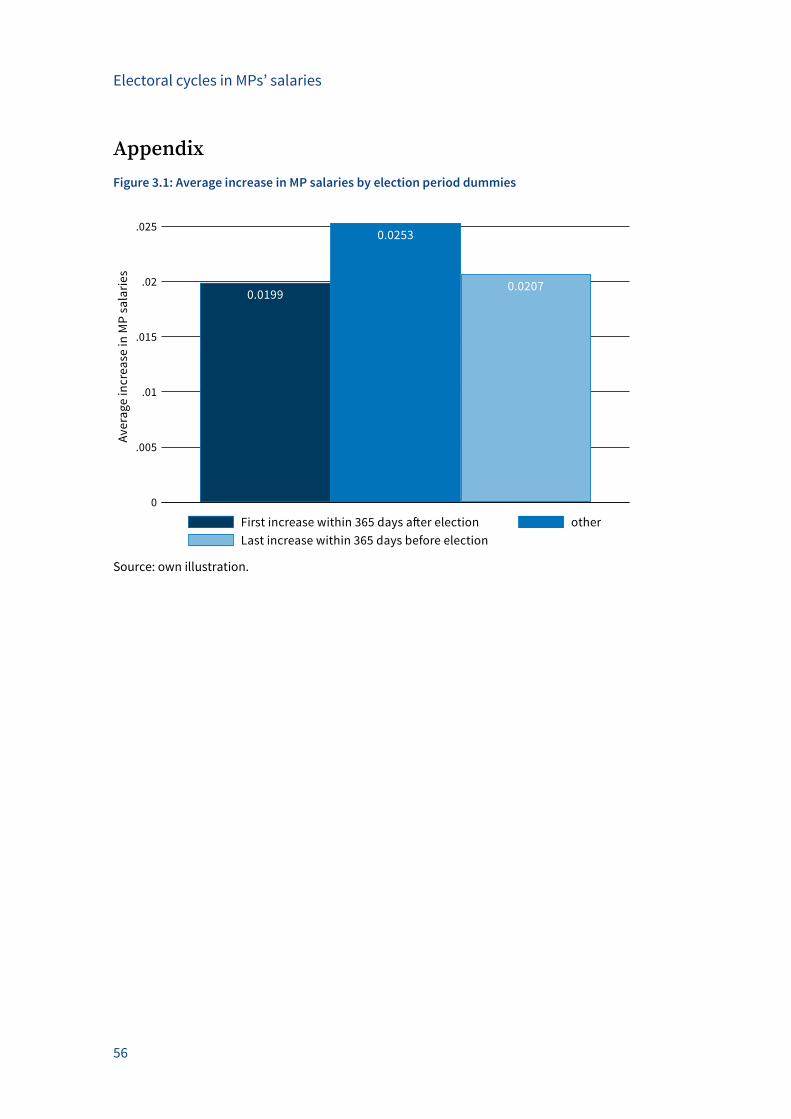
Electoral cycles in MPs’ salaries
56
Appendix
Figure 3.1: Average increase in MP salaries by election period dummies
Source: own illustration.
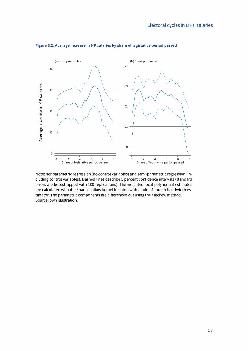
Electoral cycles in MPs’ salaries
57
Figure 3.2: Average increase in MP salaries by share of legislative period passed
Note: nonparametric regression (no control variables) and semi-parametric regression (in-
cluding control variables). Dashed lines describe 5 percent confidence intervals (standard
errors are bootstrapped with 100 replications). The weighted local polynomial estimates
are calculated with the Epanechnikov kernel function with a rule-of-thumb bandwidth es-
timator. The parametric components are differenced out using the Yatchew method.
Source: own illustration.
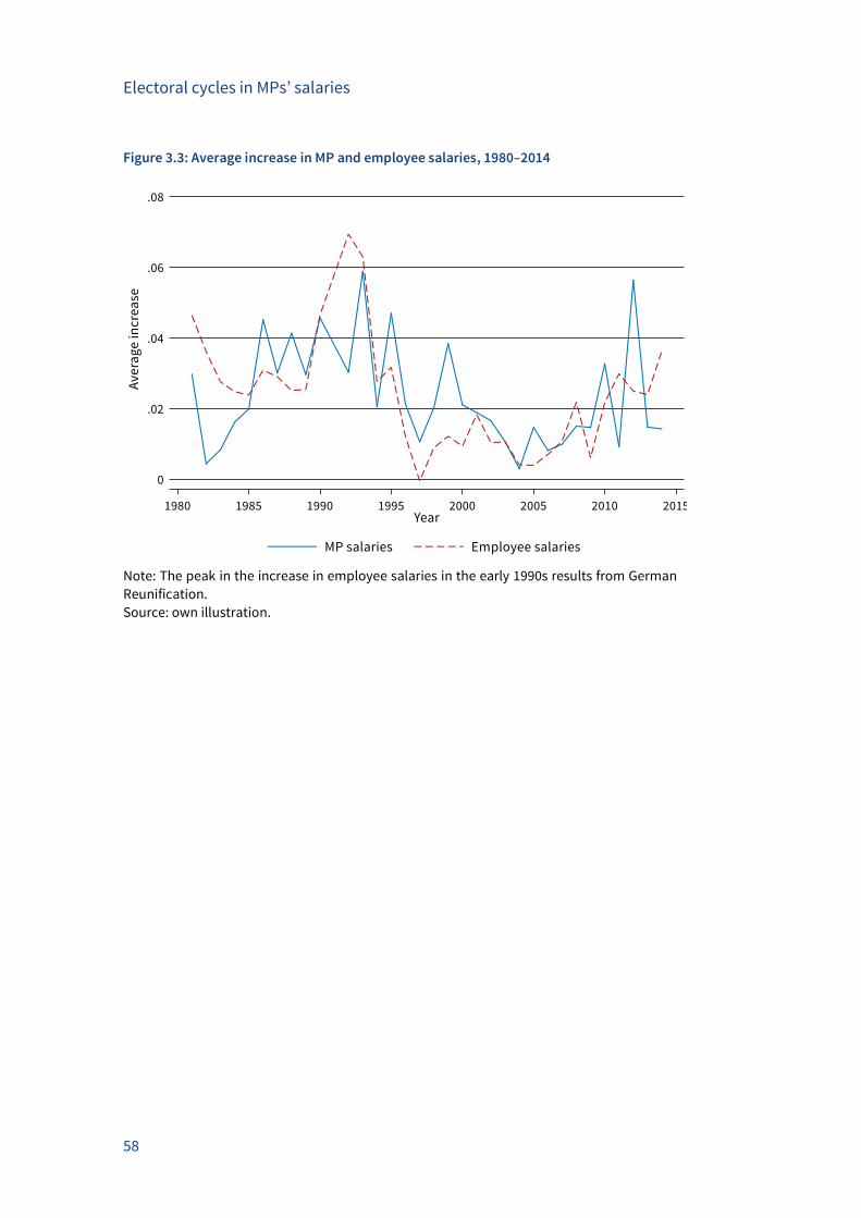
Electoral cycles in MPs’ salaries
58
Figure 3.3: Average increase in MP and employee salaries, 1980–2014
Note: The peak in the increase in employee salaries in the early 1990s results from German
Reunification.
Source: own illustration.
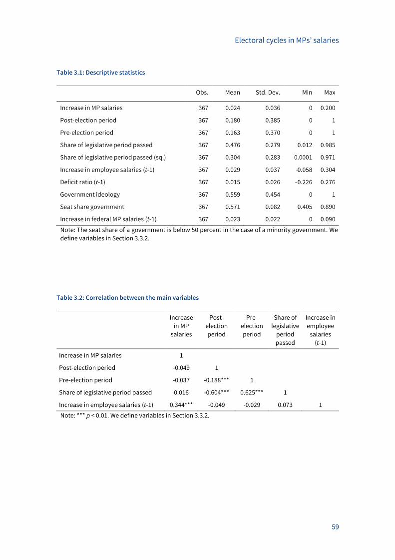
Electoral cycles in MPs’ salaries
59
Table 3.1: Descriptive statistics
Obs. Mean Std. Dev. Min Max
Increase in MP salaries 367 0.024 0.036 0 0.200
Post-election period 367 0.180 0.385 0 1
Pre-election period 367 0.163 0.370 0 1
Share of legislative period passed 367 0.476 0.279 0.012 0.985
Share of legislative period passed (sq.) 367 0.304 0.283 0.0001 0.971
Increase in employee salaries (t-1) 367 0.029 0.037 - 0.058 0.304
Deficit ratio (t-1) 367 0.015 0.026 - 0.226 0.276
Government ideology 367 0.559 0.454 0 1
Seat share government 367 0.571 0.082 0.405 0.890
Increase in federal MP salaries (t-1) 367 0.023 0.022 0 0.090
Note: The seat share of a government is below 50 percent in the case of a minority government. We
define variables in Section 3.3.2.
Table 3.2: Correlation between the main variables
Increase
in MP
salaries
Post-
election
period
Pre-
election
period
Share of
legislative
period
passed
Increase in
employee
salaries
(t-1)
Increase in MP salaries 1
Post-election period -0.049 1
Pre-election period -0.037 -0.188*** 1
Share of legislative period passed 0.016 -0.604*** 0.625*** 1
Increase in employee salaries (t-1) 0.344*** -0.049 -0.029 0.073 1
Note: *** p < 0.01. We define variables in Section 3.3.2.
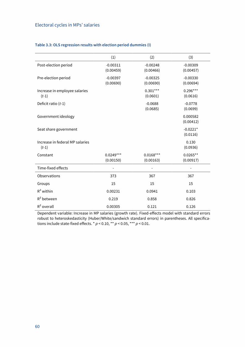
Electoral cycles in MPs’ salaries
60
Table 3.3: OLS regression results with election period dummies (I)
(1) (2) (3)
Post-election period -0.00311 -0.00248 -0.00309
(0.00459) (0.00466) (0.00457)
Pre-election period -0.00397 -0.00325 -0.00330
(0.00690) (0.00690) (0.00694)
Increase in employee salaries
(t-1)
0.301*** 0.296***
(0.0601) (0.0616)
Deficit ratio (t-1) -0.0688 -0.0778
(0.0685) (0.0699)
Government ideology 0.000582
(0.00412)
Seat share government -0.0221*
(0.0116)
Increase in federal MP salaries
(t-1)
0.130
(0.0936)
Constant 0.0249*** 0.0168*** 0.0265**
(0.00150) (0.00163) (0.00917)
Time-fixed effects - - -
Observations 373 367 367
Groups 15 15 15
R² within 0.00231 0.0941 0.103
R² between 0.219 0.858 0.826
R² overall 0.00305 0.121 0.126
Dependent variable: Increase in MP salaries (growth rate). Fixed-effects model with standard errors
robust to heteroskedasticity (Huber/White/sandwich standard errors) in parentheses. All specifica-
tions include state-fixed effects. * p < 0.10, ** p < 0.05, *** p < 0.01.
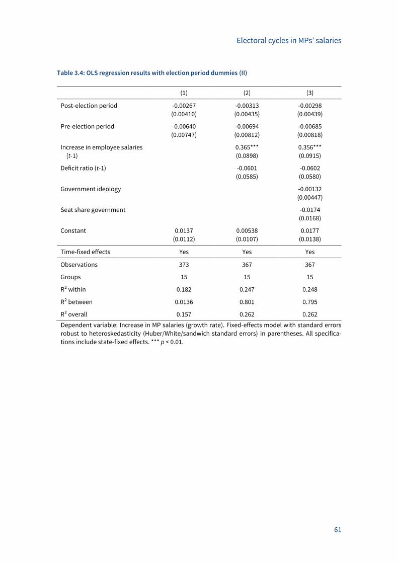
Electoral cycles in MPs’ salaries
61
Table 3.4: OLS regression results with election period dummies (II)
(1) (2) (3)
Post-election period -0.00267 -0.00313 -0.00298
(0.00410) (0.00435) (0.00439)
Pre-election period -0.00640 -0.00694 -0.00685
(0.00747) (0.00812) (0.00818)
Increase in employee salaries
(t-1)
0.365*** 0.356***
(0.0898) (0.0915)
Deficit ratio (t-1) -0.0601 -0.0602
(0.0585) (0.0580)
Government ideology -0.00132
(0.00447)
Seat share government -0.0174
(0.0168)
Constant 0.0137 0.00538 0.0177
(0.0112) (0.0107) (0.0138)
Time-fixed effects Yes Yes Yes
Observations 373 367 367
Groups 15 15 15
R² within 0.182 0.247 0.248
R² between 0.0136 0.801 0.795
R² overall 0.157 0.262 0.262
Dependent variable: Increase in MP salaries (growth rate). Fixed-effects model with standard errors
robust to heteroskedasticity (Huber/White/sandwich standard errors) in parentheses. All specifica-
tions include state-fixed effects. *** p < 0.01.
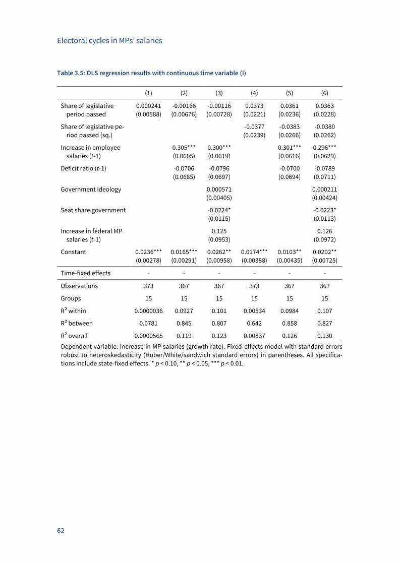
Electoral cycles in MPs’ salaries
62
Table 3.5: OLS regression results with continuous time variable (I)
(1) (2) (3) (4) (5) (6)
Share of legislative
period passed
0.000241 -0.00166 -0.00116 0.0373 0.0361 0.0363
(0.00588) (0.00676) (0.00728) (0.0221) (0.0236) (0.0228)
Share of legislative pe-
riod passed (sq.)
-0.0377 -0.0383 -0.0380
(0.0239) (0.0266) (0.0262)
Increase in employee
salaries (t-1)
0.305*** 0.300*** 0.301*** 0.296***
(0.0605) (0.0619) (0.0616) (0.0629)
Deficit ratio (t-1) -0.0706 -0.0796 -0.0700 -0.0789
(0.0685) (0.0697) (0.0694) (0.0711)
Government ideology 0.000571 0.000211
(0.00405) (0.00424)
Seat share government -0.0224* -0.0223*
(0.0115) (0.0113)
Increase in federal MP
salaries (t-1)
0.125 0.126
(0.0953) (0.0972)
Constant 0.0236*** 0.0165*** 0.0262** 0.0174*** 0.0103** 0.0202**
(0.00278) (0.00291) (0.00958) (0.00388) (0.00435) (0.00725)
Time-fixed effects - - - - - -
Observations 373 367 367 373 367 367
Groups 15 15 15 15 15 15
R² within 0.0000036 0.0927 0.101 0.00534 0.0984 0.107
R² between 0.0781 0.845 0.807 0.642 0.858 0.827
R² overall 0.0000565 0.119 0.123 0.00837 0.126 0.130
Dependent variable: Increase in MP salaries (growth rate). Fixed-effects model with standard errors
robust to heteroskedasticity (Huber/White/sandwich standard errors) in parentheses. All specifica-
tions include state-fixed effects. * p < 0.10, ** p < 0.05, *** p < 0.01.
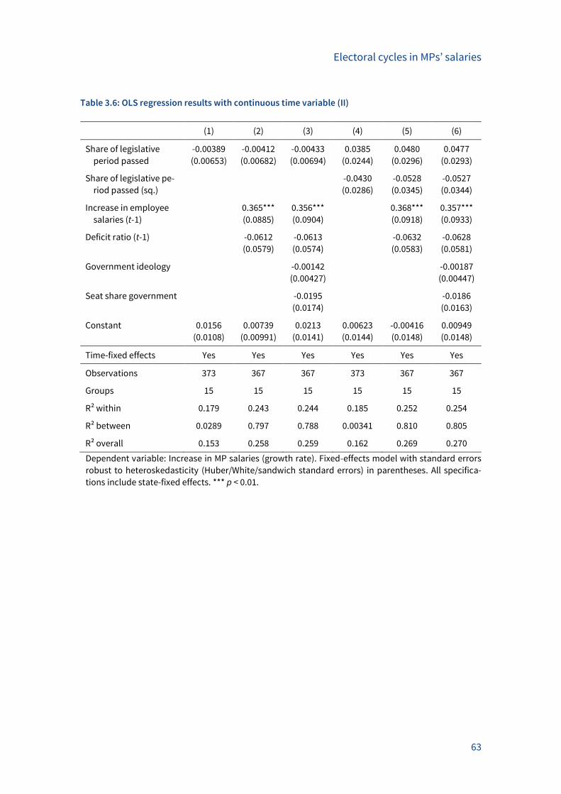
Electoral cycles in MPs’ salaries
63
Table 3.6: OLS regression results with continuous time variable (II)
(1) (2) (3) (4) (5) (6)
Share of legislative
period passed
-0.00389 -0.00412 -0.00433 0.0385 0.0480 0.0477
(0.00653) (0.00682) (0.00694) (0.0244) (0.0296) (0.0293)
Share of legislative pe-
riod passed (sq.)
-0.0430 -0.0528 -0.0527
(0.0286) (0.0345) (0.0344)
Increase in employee
salaries (t-1)
0.365*** 0.356*** 0.368*** 0.357***
(0.0885) (0.0904) (0.0918) (0.0933)
Deficit ratio (t-1) -0.0612 -0.0613 -0.0632 -0.0628
(0.0579) (0.0574) (0.0583) (0.0581)
Government ideology -0.00142 -0.00187
(0.00427) (0.00447)
Seat share government -0.0195 -0.0186
(0.0174) (0.0163)
Constant 0.0156 0.00739 0.0213 0.00623 -0.00416 0.00949
(0.0108) (0.00991) (0.0141) (0.0144) (0.0148) (0.0148)
Time-fixed effects Yes Yes Yes Yes Yes Yes
Observations 373 367 367 373 367 367
Groups 15 15 15 15 15 15
R² within 0.179 0.243 0.244 0.185 0.252 0.254
R² between 0.0289 0.797 0.788 0.00341 0.810 0.805
R² overall 0.153 0.258 0.259 0.162 0.269 0.270
Dependent variable: Increase in MP salaries (growth rate). Fixed-effects model with standard errors
robust to heteroskedasticity (Huber/White/sandwich standard errors) in parentheses. All specifica-
tions include state-fixed effects. *** p < 0.01.
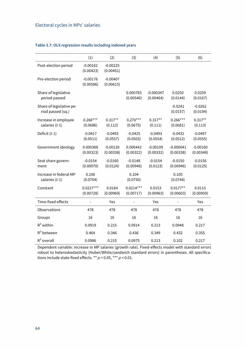
Electoral cycles in MPs’ salaries
64
Table 3.7: OLS regression results including indexed years
(1) (2) (3) (4) (5) (6)
Post-election period -0.00162 -0.00225
(0.00423) (0.00451)
Pre-election period -0.00176 -0.00407
(0.00586) (0.00615)
Share of legislative
period passed
0.000783 -0.000347 0.0250 0.0259
(0.00546) (0.00464) (0.0144) (0.0167)
Share of legislative pe-
riod passed (sq.)
-0.0241 -0.0262
(0.0157) (0.0194)
Increase in employee
salaries (t-1)
0.268*** 0.317** 0.270*** 0.317** 0.266*** 0.317**
(0.0686) (0.112) (0.0675) (0.111) (0.0681) (0.113)
Deficit (t-1) -0.0417 -0.0493 -0.0425 -0.0493 -0.0432 -0.0497
(0.0511) (0.0557) (0.0503) (0.0554) (0.0512) (0.0555)
Government ideology 0.000368 -0.00120 0.000442 -0.00109 -0.000041 -0.00160
(0.00323) (0.00338) (0.00322) (0.00332) (0.00338) (0.00348)
Seat share govern-
ment
-0.0154 -0.0160 -0.0148 -0.0154 -0.0150 -0.0156
(0.00970) (0.0124) (0.00946) (0.0123) (0.00946) (0.0125)
Increase in federal MP
salaries (t-1)
0.106 0.104 0.105
(0.0704) (0.0750) (0.0744)
Constant 0.0227*** 0.0164 0.0214*** 0.0153 0.0177** 0.0115
(0.00728) (0.00969) (0.00717) (0.00963) (0.00603) (0.00959)
Time-fixed effects - Yes - Yes - Yes
Observations 478 478 478 478 478 478
Groups 16 16 16 16 16 16
R² within 0.0919 0.215 0.0914 0.213 0.0948 0.217
R² between 0.464 0.346 0.436 0.349 0.432 0.355
R² overall 0.0986 0.215 0.0975 0.213 0.102 0.217
Dependent variable: Increase in MP salaries (growth rate). Fixed-effects model with standard errors
robust to heteroskedasticity (Huber/White/sandwich standard errors) in parentheses. All specifica-
tions include state-fixed effects. ** p < 0.05, *** p < 0.01.
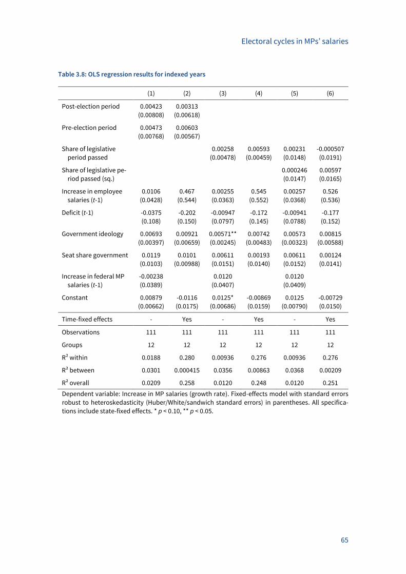
Electoral cycles in MPs’ salaries
65
Table 3.8: OLS regression results for indexed years
(1) (2) (3) (4) (5) (6)
Post-election period 0.00423 0.00313
(0.00808) (0.00618)
Pre-election period 0.00473 0.00603
(0.00768) (0.00567)
Share of legislative
period passed
0.00258 0.00593 0.00231 -0.000507
(0.00478) (0.00459) (0.0148) (0.0191)
Share of legislative pe-
riod passed (sq.)
0.000246 0.00597
(0.0147) (0.0165)
Increase in employee
salaries (t-1)
0.0106 0.467 0.00255 0.545 0.00257 0.526
(0.0428) (0.544) (0.0363) (0.552) (0.0368) (0.536)
Deficit (t-1) -0.0375 -0.202 -0.00947 -0.172 -0.00941 -0.177
(0.108) (0.150) (0.0797) (0.145) (0.0788) (0.152)
Government ideology 0.00693 0.00921 0.00571** 0.00742 0.00573 0.00815
(0.00397) (0.00659) (0.00245) (0.00483) (0.00323) (0.00588)
Seat share government 0.0119 0.0101 0.00611 0.00193 0.00611 0.00124
(0.0103) (0.00988) (0.0151) (0.0140) (0.0152) (0.0141)
Increase in federal MP
salaries (t-1)
-0.00238 0.0120 0.0120
(0.0389) (0.0407) (0.0409)
Constant 0.00879 -0.0116 0.0125* -0.00869 0.0125 -0.00729
(0.00662) (0.0175) (0.00686) (0.0159) (0.00790) (0.0150)
Time-fixed effects - Yes - Yes - Yes
Observations 111 111 111 111 111 111
Groups 12 12 12 12 12 12
R² within 0.0188 0.280 0.00936 0.276 0.00936 0.276
R² between 0.0301 0.000415 0.0356 0.00863 0.0368 0.00209
R² overall 0.0209 0.258 0.0120 0.248 0.0120 0.251
Dependent variable: Increase in MP salaries (growth rate). Fixed-effects model with standard errors
robust to heteroskedasticity (Huber/White/sandwich standard errors) in parentheses. All specifica-
tions include state-fixed effects. * p < 0.10, ** p < 0.05.

Electoral cycles in MPs’ salaries
66
Do left-wing governments decrease income inequality?
67
4 Do left-wing governments decrease income
inequality? Empirical evidence based on
salaries of civil servants
Do left-wing governments decrease income inequality?
Abstract*
We investigate whether left-wing governments decrease income inequality. The data is based
on salaries of German civil servants. Since a reform in 2006, German state governments are
allowed to design salaries of civil servants. We employ encompassing data for pay levels and
professions including judges, professors, policemen, and administrators and distinguish be-
tween levels of operating experiences. We use five income inequality measures comparing
salaries across pay levels and operating experiences. The results do not suggest that left-wing
governments were more active in decreasing income inequality than center or right-wing gov-
ernments. Cabinet members are civil servants themselves and decide on their own salaries:
government ideology is also not shown to predict salaries of cabinet members. Because left-
wing governments are perceived as taking action against income inequality, future research
should employ data from other federal states such as the United States to examine how gov-
ernment ideology influences salaries of civil servants.
* This chapter is joint work with Björn Kauder and Niklas Potrafke. Isaac N. Cohen, Christina Dannhorn, Kristin Fischer, and Felix
Michalik provided excellent research assistance.
Do left-wing governments decrease income inequality?
68
Introduction
Income inequality has decreased across countries but is still pronounced within many coun-
tries. Scholars examine what influences income inequality across and within countries. A
prominent example is globalization (Dreher and Gaston 2008, Bergh and Nilsson 2010, Dorn
et al. 2017, Lang and Tavares 2018). Clearly, domestic governments have a hard time to pre-
vent globalization influencing income inequality, especially when they wish to enjoy benefits
of globalization and do not protect their economies from trade and foreign investment flows.
Domestic governments may well, however, respond to globalization and its effects on income
inequality by implementing policies such as increasing social expenditure, regulating labor
markets, and increasing taxes for high-income citizens. The extent to which domestic govern-
ments wish to address income inequality and be active in income redistribution is likely to
depend on government ideology. Left-wing governments are expected to be more active in
income redistribution to decrease income inequality than right-wing governments. Empirical
evidence shows that top income shares increased under right-wing governments more rapidly
than under left-wing governments (Scheve and Stavasage 2009, Dorn and Schinke 2018). The
previous studies examining how government ideology influences income inequality used
panel data for OECD countries and univariate times series for individual OECD countries.
We examine how government ideology influences within-country income inequality. We em-
ploy new data on civil servants’ salaries that encompass variation across pay levels and oper-
ating experiences. The sample includes salaries of all civil servants in the German states:
judges, professors, policemen, administrators etc. We elaborate on a reform of the German
fiscal constitution in 2006: the reform allowed German state governments to design salaries
of civil servants. The results do not suggest that left-wing governments were more active in
decreasing income inequality among civil servants than center or right-wing governments.
Background and hypothesis
4.2.1 Government ideology and income redistribution
Left-wing governments are expected to increase the size and scope of governments and, in
turn, to decrease income inequality. The partisan theories describe that both left-wing and
right-wing governments gratify the needs of their constituencies (Hibbs 1977, Chappell and
Keech 1986, Alesina 1987). Blue-collar workers, low-income, and low-skilled citizens have
been the constituency of left-wing parties, and self-employed, high-income, and high-skilled
citizens have been the constituency of right-wing parties for a long time. The partisan theories
modelled the economy by a Phillips curve tradeoff: politicians use fiscal and monetary poli-
cies to choose between unemployment and inflation. Left-wing governments that cater the
interests of low-income citizens will implement expansionary fiscal and monetary policies to
keep unemployment low (and accept inflation). Right-wing governments cater the interests
Do left-wing governments decrease income inequality?
69
of high-income citizens; they will implement restrictive fiscal and monetary policies to keep
inflation at low rates (and accept unemployment).
The partisan theories have been translated to many economic policy fields; the core hypoth-
esis to be investigated being that left-wing governments increase the size and scope of gov-
ernment which includes income redistribution from high-income to low-income citizens (for
surveys see Schmidt 1996, Potrafke 2017, Zohlnhöfer et al. 2018). Governments have manifold
measures at hand to redistribute income from high-income to low-income citizens. An im-
portant measure is to tax high-income citizens to a large extent. Taxing high-income citizens
incorporates progressive income taxation. Marginal tax rates should be much higher for high
than for low incomes, and governments may well grant generous tax-exempt amounts for low
incomes. Because high-income citizens often enjoy pronounced capital incomes, govern-
ments advocating income redistribution are likely to tax capital more progressively than la-
bor. Low-income citizens usually spend a large amount of their income for consumption. One
would therefore expect that left-wing governments are less active in increasing consumption
tax rates than right-wing governments. Empirical evidence for OECD countries tends to con-
firm ideology-induced tax policies (e.g., Angelopoulous et al. 2012, Osterloh and Debus 2012).
Income redistribution also includes generous transfers to low-income citizens. A prominent
example is social policies. Left-wing governments may want to promote social insurance
against risks such as illness, old age, and unemployment to attract poorer voters and voters
with larger health risks (De Donder and Hindriks 2007). Encompassing social insurance gives
rise to increasing social expenditure. Scholars have examined how government ideology in-
fluences social expenditure. The empirical evidence for OECD countries suggests that social
expenditure was higher under left-wing governments until the end of the 1980s; government
ideology retired to the background in the 1990s and early 2000s. New studies report ideology-
induced social policies, the fields of social policy (health, old age, active labor market policies
etc.) notwithstanding.1
Pronounced social spending and progressive taxation under left-wing governments accom-
panied decreasing income inequality. The studies by Scheve and Stavasage (2009) and Dorn
and Schinke (2018) show that top income shares were higher under right-wing than under left-
wing governments.2 The governments of Margaret Thatcher in the United Kingdom and
Ronald Reagan in the United States were prime examples for market-oriented policies in the
1980s. The policies included deregulation of labor and product markets, privatizations of
state-owned companies and cutting social expenditure and tax reliefs especially for high-in-
come citizens. The top one percent income share started to drastically increase when
1 See, for example, Potrafke (2009 and 2017), Bove et al. (2017), Herwartz and Theilen (2017), Savage (2018), and Schuknecht and
Zemanek (2018).
2 See Bjørnskov (2008) on the nexus between government ideology, income inequality, and economic growth in developing coun-
tries.
Do left-wing governments decrease income inequality?
70
Thatcher and Reagan came into power. After the 1980s, however, government ideology was
not related with top income shares in Anglo-Saxon countries, but in many other OECD coun-
tries.
We expect left-wing governments to be more active in reducing income inequality than center
and right-wing governments.
4.2.2 Ideology-induced policies in the German states
Examining ideology-induced income redistribution – especially within countries – requires
some more fine-grained data than previous studies used. We focus on the German states in
which government ideology has been shown to influence economic policies.
German state governments have room to maneuver in individual policy fields such as educa-
tion and cultural policies. Right-wing governments spent more on universities and somewhat
less on primary schools and were more active in introducing tuition fees than left-wing gov-
ernments (Oberndorfer and Steiner 2007, Potrafke 2011, Kauder and Potrafke 2013). Law and
order policies were influenced by government ideology: right-wing governments hired more
policemen and used dragnet-controls – controls of persons conducted by the police without
having any suspicion that the controlled person committed a crime – more often than left-
wing governments (Tepe and Vanhuysse 2013, Potrafke 2018). German state governments
have hardly any means in designing tax policies. An exception is the real-estate transfer tax:
the fiscal constitution was reformed in 2006 and allowed state governments to set real-estate
transfer tax rates. Empirical evidence shows that left-wing and center governments were
more active in increasing the real-estate transfer tax rates than right-wing governments
(Krause and Potrafke 2017 – see Chapter 5). Left-wing governments that increase real-estate
transfer tax rates may well be inclined to redistribute income from high-income to low-income
citizens because high-income citizens are more likely to buy properties than low-income citi-
zens and, in turn, pay real-estate transfer taxes.
Left-wing governments may well use salaries of public employees to redistribute incomes: sal-
aries of low-skilled public employees are expected to increase to a larger extent than salaries
of high-skilled public employees. Especially well-paid public employees are judges and cabi-
net members of state governments (in Germany, all of them are civil servants and enjoy also
other benefits such as entitlements to a pension). Many well-paid public employees receive
high salaries in old age, when retirement is close. A reason is experience and networking that
are required for job promotion. Another reason is that salaries of public employees mechani-
cally increase – without any job promotion – over time. The German law rewards operating
experience. Low-paid public employees do services in the administration such as errands.
Clearly, many low-paid public employees are young and therefore receive quite low salaries
because they are both grouped into a low pay level and do not have much operating experi-
ence yet. It is conceivable that low-paid public employees are likely to vote for left-wing par-
Do left-wing governments decrease income inequality?
71
ties that may want to increase entry-level salaries. In a similar vein, well-paid public employ-
ees are likely to vote for right-wing parties that are, in turn, inclined to further reward well-
paid public employees.
State governments have many means to influence income redistribution among public em-
ployees. First, governments design the vertical distribution of pay levels by changing, for ex-
ample, the relation between salaries of a judge in a local court and a chief judge in the su-
preme court. Second, governments design the horizontal distribution of pay levels by
changing, for example, the relation between salaries of a judge in a local court with 2 and 30
years of operating experience.
We expect left-wing governments to compress the distribution of salaries of public employees
more than right-wing governments. We also expect left-wing governments to increase entry-
level salaries more than top salaries.
Institutional backdrop
4.3.1 Salaries of civil servants
In September 2006, a large reform of German federalism took effect. One of the key elements
of the reform was the decision that state parliaments are allowed to set salaries of their civil
servants. Before the reform, the salaries of all German civil servants were decided on at the
federal level. The first state that set its own salaries was Bavaria in 2007. Most other states
followed in 2008.
In all states, civil servants are paid based on five pay-level groups (see Table 4.1). Most civil
servants are paid on the A-level, upper-level civil servants on the B-level, professors on the C-
and the W-level, and judges and prosecutors on the R-level. Within each of these groups there
are different individual pay levels. For example, A-level civil servants are paid a salary on the
levels A2 to A16 and R-level civil servants on the levels R1 to R10. Within each of these pay
levels, there are in turn different levels of operating experience. C-level civil servants, for ex-
ample, are categorized into up to 15 different levels of operating experience.
4.3.2 The German political party landscape
Two major political parties have characterized the political landscape in Germany: the leftist
Social Democratic Party (SPD) and the conservative Christian Democratic Union (CDU; in Ba-
varia CSU). All federal chancellors and state prime ministers – except the green prime minister
of Baden-Wuerttemberg elected in 2011 and the prime minister of Thuringia from the Left
Party elected in 2014 – were members of one of these two parties, SPD and CDU. We can there-
fore test for ideology-induced policy-making on a left-right scale.
Do left-wing governments decrease income inequality?
72
The Free Democratic Party (FDP) and the Greens (Bündnis 90/Die Grünen) – both much smaller
– have played an important role as coalition partners in the West German states, the Left Party
(Die Linke) as coalition partner in the East German states.
Empirical analysis
4.4.1 Empirical strategy
State governments decide on increasing salaries of civil servants quite erratically, at seem-
ingly arbitrary points in time. Only in some cases, state governments increase salaries regu-
larly year after year. State governments also often decide on multiple salary increases at the
same time. Many decisions include, for example, an increase with retroactive effect from the
beginning of the current year, and two increases effective from the beginning of the next year
and the beginning of the year after the next year. This erratic pattern makes it infeasible to
estimate panel data models using annual data on salary increases. Following Schmitt (2015),
we thus condense our data and examine legislative periods.
The baseline panel-data model has the following form:
Change in measure of salariesi,t = β Government ideologyi,t + γ Seat share governmenti,t
+ δ l.Increase in employee salariesi,t + ε l.Increase in Gini of employee salariesi,t
+ ζ l.Increase in debt/GDPi,t + θ l.Increase in civil servants p.c.i,t
+ φ l.Change in measure of salaries (federal)i,t + ηi + τt + ui,t
with i = 1,…,16; t = 2007,…,2017 (median year of legislative period; unbalanced)
where Change in measure of salariesi,t describes five measures of average annual growth in
inequality and two different measures of nominal salaries’ growth in state i in the legislative
period with median year t. Table 4.1 shows one of the 225 salary scales in our data set as an
example. We use all salary scales passed by an individual government to calculate the growth
or growth in inequality per year of a legislative period. The individual rows show different pay
levels, and the individual columns show different levels of operating experience. Increase in
diagonal inequalityi,t is a cross-section type of inequality measure and describes the growth
rate of the relation between the highest and the lowest salary in a salary scale. Increase in
vertical inequalityi,t describes the growth rate of the relation between the highest and the low-
est salary among those civil servants that have reached the highest level of operating experi-
ence (technically speaking: the growth rate of the relation between the highest and the lowest
row maximum). It is thus an individual-specific measure of inequality, because all civil serv-
ants will basically reach the highest level of operating experience at some time. Increase in
horizontal inequalityi,t first calculates the relation between the salaries of the highest and of
the lowest level of operating experience for every individual pay level, and then calculates the
average of the resulting relations. The measure thus describes the extent to which experience
Do left-wing governments decrease income inequality?
73
is remunerated. Increase in horizontal inequality (weighted)i,t follows the same idea, does how-
ever weight the individual pay scales according to the number of civil servants in these pay
scales.3 Increase in Gini coefficienti,t describes how the Gini coefficient of salaries has increased.
Information on the number of civil servants in the individual levels of operating experience is
not available. The measure thus assumes that all civil servants have reached the highest level
of operating experience, and again uses weights for the number of civil servants in the indi-
vidual pay scales. Average growthi,t describes the average of the growth rates of the mean sal-
aries in the individual pay scales (note that calculating growth rates of all cells in the salary
scale individually is not feasible, because the number of levels of operating experience
changes quite often). Average growth (weighted)i,t alters this measure by using weights of the
number of civil servants in the individual pay scales when calculating the average.
The variable Government ideologyi,t measures ideology-induced policy-making and takes on
the value 1 when a left-wing government is in office, the value 0.5 for a center government,
and the value 0 for a right-wing government (e.g., Kauder and Potrafke 2013, Potrafke et al.
2016). In alternative specifications, we also use dummy variables for left-wing, center, and
right-wing governments, because the government ideology index assumes a linear relation-
ship between the individual types of governments. We expect that left-wing governments de-
crease inequality. The effect of government ideology on the growth of salaries is however not
clear. Left-wing governments prefer a larger size of government than do right-wing govern-
ments and should thus increase salaries more. Some civil servants, such as judges, are how-
ever not core constituencies of left-wing governments and should thus not be expected to
enjoy large increases in salaries. It is conceivable that politicians increase salaries for civil
servants more when their party holds a large majority of seats in parliament (see Benito et al.
2014, Svaleryd and Vlachos 2009). Seat share governmenti,t thus measures the number of seats
the governing parties have relative to all seats in parliament.
We include five control variables that we measure with a lag of one year. For example, if a
legislative period lasts from March 2011 through March 2016, we consider the control variable
in the period from March 2010 through March 2015.4 All these variables are calculated as per
year of the legislative period’s length. l.Increase in employee salariesi,t measures the extent to
which nominal salaries of public- and private-sector employees increased in a state (see also
Di Tella and Fisman 2004). We expect the salaries of private- and public-sector employees to
be positively correlated with salaries of civil servants. The effect on inequality is however the-
oretically ambiguous. l.Increase in Gini of employee salariesi,t describes the increase in the Gini
3 Data on the number of civil servants in individual pay scales is only available from 2011 through 2016. We thus use the 2011
weights also for all years before 2011, and the 2016 weights also for 2017 and 2018. Weights are identical over all states, also
because of data availability.
4 In this example, the year 2010 enters the calculation with a weight of 9.5/12 (months), and the year 2015 with a weight of 2.5/12
(months), if the legislative period ends and begins in the middle of March. The years 2011–2014 enter with a full weight of 12/12.
Do left-wing governments decrease income inequality?
74
coefficient of private- and public-sector employees in a state. Here we expect a positive cor-
relation with inequality of civil servants’ salaries, whereas the correlation with the growth of
salaries is unclear. The variable l.Increase in debt/GDPi,t measures how public debt in a state
has increased relative to state’s GDP. We expect this variable to be negatively correlated with
salaries of civil servants because state governments are unlikely to increase salaries of civil
servants when public debt is increasing. l.Increase in civil servants p.c.i,t measures the extent
to which the number of state civil servants per capita has increased. The correlation with our
dependent variables is theoretically ambiguous.5 Finally, we include the dependent variables
as measured for salaries of civil servants on the federal level (e.g., the increase in the Gini co-
efficient of federal civil servants), which may serve as a benchmark for state policy-makers
when deciding on the salaries of state civil servants. ηi is a fixed state effect; τt is a fixed time
effect (based on the median year of a legislative period; reference category: 2007); ui,t is the
error term. We estimate the fixed-effects model with standard errors robust to heteroskedas-
ticity (Huber/White/sandwich standard errors; see Huber 1967, White 1980).
4.4.2 Descriptive statistics
Figure 4.1 shows the means of our dependent variables separately for left-wing, center, and
right-wing governments. The upper two panels show that in legislative periods with a right-
wing government, diagonal and vertical inequality decreased by about 1.6 percent per year.
Under left-wing and center governments, by contrast, diagonal and vertical inequality de-
creased by only about half a percent per year. Horizontal inequality, measuring how much
experience is remunerated, and the Gini coefficient show only values smaller than one percent
for left-wing, center, and right-wing governments. The average growth rates of salaries hardly
differ between left-wing, center, and right-wing governments. For all types of governments,
growth rates are on average about 2.5 to 3 percent. Table 4.2 shows descriptive statistics. Ta-
ble 4.3 contains the correlation coefficients between our main variables. The bottom row in-
dicates that left-wing governments were more active in increasing diagonal and vertical ine-
quality, and less active in increasing horizontal inequality, and insofar corroborates the
evidence from Figure 4.1. Our data set includes 50 observations.6
4.4.3 Regression results
Table 4.4 shows the regression results of the baseline model when fixed state but no fixed time
effects are included. The variable Government ideology does not turn out to be statistically
significant in Columns (2) to (7), it is statistically significant at the 10 percent level with an
unexpected positive sign in Column (1). The coefficient estimate of the variable Government
5 Data on the number of civil servants in the individual states is only available until 2016. We thus use the value for 2016 also for
2017.
6 Note that there is one legislative period in the data set without a decision on salaries (Saarland 2009–2012). We code the date
of decision of this non-increase as the exact middle of the legislative period. We also included legislative periods that have
started, but not yet ended until the end of our data set (February 2018), when either a decision on salaries has already taken
place or the period was running for at least one year.
Do left-wing governments decrease income inequality?
75
ideology indicates that the growth rate in diagonal civil servant salary inequality increased by
around 0.9 percentage points when the government ideology variable increased by one point,
that is from a right-wing to a left-wing government.
Some of the control variables help to predict increases in inequality of civil servants’ salaries
and are statistically significant. Increases in the Gini of employee salaries are, for example,
positively correlated with increases in horizontal inequality of civil servants’ salaries (Columns
3 and 4). Increases in horizontal inequality of civil servants’ salaries at the federal level are
positively correlated with increases in horizontal inequality of civil servants’ salaries at the
state level (Column 3). The average weighted growth of salaries at the federal level is also pos-
itively correlated with the average weighted growth of salaries at the state level (Column 7).
When we include fixed time effects (Table 4.5), the point estimate of the variable Government
ideology in Column (1) remains positive but lacks statistical significance. By contrast, the point
estimate of the variable Government ideology in Column (3) renders to be statistically signifi-
cant at the 5 percent level indicating that the growth rate in horizontal inequality of civil serv-
ants’ salaries decreased by around 0.3 percentage points when the government ideology var-
iable increased by one point, that is from a right-wing to a left-wing government. The estimate
of the variable Government ideology in Column (4) does however not suggest that the growth
rate in horizontal inequality of civil servants’ salaries decreased under left-wing governments
once we weight the individual pay scales according to the number of civil servants in these
pay scales. In fact, it slightly fails to be statistically significant at the 10 percent level.
Table 4.6 shows the results when we include dummy variables for left-wing and center gov-
ernments (reference category: right-wing governments), to allow for a non-linear relationship
between the individual types of government ideology. Inferences do not change compared to
Table 4.5. The dummy variable Ideology left is only statistically significant at the 10 percent
level when Increase in horizontal inequality is the dependent variable. The dummy variable
Ideology center does not turn out to be statistically significant in any specification.
4.4.4 Robustness tests
We submitted our results to rigorous robustness tests using different specifications of our re-
gressions and different samples. None of these robustness tests indicates any severe fragility
in our results.
Ideology-induced policy-making has been shown to differ between East and West German
states (see, for example, Potrafke 2013 and Kauder et al. 2017). When replicating Table 4.5 for
West German states only, the results do not show that government ideology influenced any of
our dependent variables, except for the increase in horizontal inequality (negative and statis-
tically significant at the 10 percent level). Running the model only for East German states is
not meaningful because of only 15 observations.
Do left-wing governments decrease income inequality?
76
We tested whether inferences differ across individual pay-level groups (A, B, C, R, and W) by
again replicating Table 4.5. In pay-level group A (including most civil servants), the variable
Government ideology shows a positive and statistically significant effect for the weighted in-
crease in horizontal inequality. In pay-level group C (including professors), government ideol-
ogy is positively associated with the variable Average growth (statistically significant at the 10
percent level). For the other dependent variables and pay-level groups, government ideology
does not turn out to be statistically significant.
In the baseline model, all dependent variables are calculated as per year of the legislative pe-
riod’s length. Replicating Table 4.5, inferences hardly change when we calculate the depend-
ent variables as per year of how long increases are valid: the effect of government ideology is
positive and now statistically significant at the 10 percent level when Average growth is the
dependent variable.
Salaries of cabinet members
Why is it that left-wing governments are not shown to be more active in decreasing inequality
of civil servants than center and right-wing governments? It is conceivable that they have self-
interests because all cabinet members are employed as (temporary) civil servants them-
selves.7 Cabinet members receive B10 or B11 salaries (the highest B pay level) plus a percent-
age premium on top of B10 or B11. The percentage premia are decided by the state parliament
in which the parties of the state governments have a majority.8 Table 4.7 shows that there is
quite some variation in the percentage premia across the German states. In 2017, for example,
the percentage premium in Bremen was actually zero – the only German state which did not
grant any premium. In North Rhine-Westphalia, the premium was 33 percent for the prime
minister. Table 4.7 shows however also that there is hardly any variation within states. Only
in few cases, governments increased or decreased the percentage premium for prime minis-
ters or ministers between 2007 and 2017. Decreases occurred under a right-wing government
in Hesse, a left-wing government in Rhineland-Palatinate, a center government in Schleswig-
Holstein, and a right-wing government in Thuringia. A center government in Thuringia in-
creased salaries of cabinet members. This case study evidence does not suggest that govern-
ment ideology influenced salaries of cabinet members.
We have also estimated our baseline model excluding the pay levels B10 and B11, and the
entire B-level. Inferences regarding the effects of government ideology do not change.
7 On electoral cycles in salaries of US federal bureaucrats and German state members of parliament see Borjas (1984) and Kauder
et al. (2018) – see Chapter 3.
8 There is only one minority government in our sample (North Rhine-Westphalia 2010–2012). To be sure, formally there were
further minority governments, which however existed only for quite short periods, after coalition governments failed and new
elections were called.
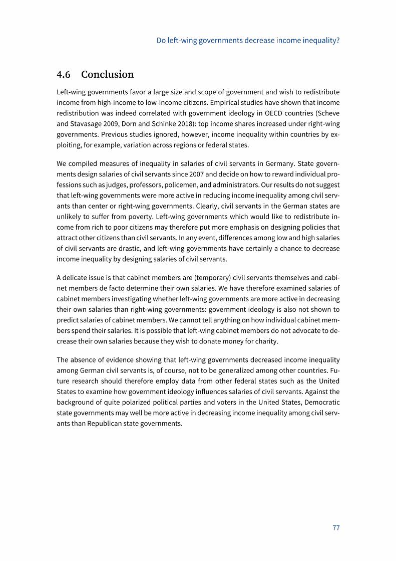
Do left-wing governments decrease income inequality?
77
Conclusion
Left-wing governments favor a large size and scope of government and wish to redistribute
income from high-income to low-income citizens. Empirical studies have shown that income
redistribution was indeed correlated with government ideology in OECD countries (Scheve
and Stavasage 2009, Dorn and Schinke 2018): top income shares increased under right-wing
governments. Previous studies ignored, however, income inequality within countries by ex-
ploiting, for example, variation across regions or federal states.
We compiled measures of inequality in salaries of civil servants in Germany. State govern-
ments design salaries of civil servants since 2007 and decide on how to reward individual pro-
fessions such as judges, professors, policemen, and administrators. Our results do not suggest
that left-wing governments were more active in reducing income inequality among civil serv-
ants than center or right-wing governments. Clearly, civil servants in the German states are
unlikely to suffer from poverty. Left-wing governments which would like to redistribute in-
come from rich to poor citizens may therefore put more emphasis on designing policies that
attract other citizens than civil servants. In any event, differences among low and high salaries
of civil servants are drastic, and left-wing governments have certainly a chance to decrease
income inequality by designing salaries of civil servants.
A delicate issue is that cabinet members are (temporary) civil servants themselves and cabi-
net members de facto determine their own salaries. We have therefore examined salaries of
cabinet members investigating whether left-wing governments are more active in decreasing
their own salaries than right-wing governments: government ideology is also not shown to
predict salaries of cabinet members. We cannot tell anything on how individual cabinet mem-
bers spend their salaries. It is possible that left-wing cabinet members do not advocate to de-
crease their own salaries because they wish to donate money for charity.
The absence of evidence showing that left-wing governments decreased income inequality
among German civil servants is, of course, not to be generalized among other countries. Fu-
ture research should therefore employ data from other federal states such as the United
States to examine how government ideology influences salaries of civil servants. Against the
background of quite polarized political parties and voters in the United States, Democratic
state governments may well be more active in decreasing income inequality among civil serv-
ants than Republican state governments.
Do left-wing governments decrease income inequality?
78
References
Alesina, A. (1987). Macroeconomic policy in a two-party system as a repeated game. Quarterly
Journal of Economics, 102, 651–678.
Angelopoulos, K., G. Economides, and P. Kammas (2012). Does cabinet ideology matter for the
structure of tax policies? European Journal of Political Economy, 28, 620–635.
Benito, B., F. Bastida, A.-M. Ríos, and C. Vicente (2014). The causes of legal rents extraction:
Evidence from Spanish municipalities. Public Choice, 161, 367–383.
Bergh, A. and T. Nilsson (2010). Do liberalization and globalization increase income inequal-
ity? European Journal of Political Economy, 26, 488–505.
Bjørnskov, C. (2008). The growth-inequality association: Government ideology matters. Jour-
nal of Development Economics, 87, 300–308.
Borjas, G. (1984). Electoral cycles and the earnings of federal bureaucrats. Economic Inquiry,
22, 447–459.
Bove, V., G. Efthyvoulou, and A. Navas (2017). Political cycles in public expenditure: Butter vs
guns. Journal of Comparative Economics, 45, 582–604.
Chappell, H. W. Jr. and W. R. Keech (1986). Party differences in macroeconomic policies and
outcomes. American Economic Review, 76, 71–74.
De Donder, P. and J. Hindriks (2007). Equilibrium social insurance with policy-motivated par-
ties. European Journal of Political Economy, 23, 624–640.
Di Tella, R. and R. Fisman (2004). Are politicians really paid like bureaucrats? Journal of Law
and Economics, 47, 477–513.
Dorn, F., C. Fuest, and N. Potrafke (2017). Globalisation and income inequality revisited. Euro-
pean Commission Discussion Paper 056.
Dorn, F. and C. Schinke (2018). Top income shares in OECD Countries: The role of government
ideology and globalization. World Economy, 41, 2491–2527.
Dreher, A. and N. Gaston (2008). Has globalisation increased inequality? Review of Interna-
tional Economics, 16, 516–536.
Herwartz, H. and B. Theilen (2017). Ideology and redistribution through public spending. Eu-
ropean Journal of Political Economy, 46, 74–90.
Hibbs, D. A. Jr. (1977). Political parties and macroeconomic policy. American Political Science
Review, 71, 1467–1487.
Huber, P. J. (1967). The behavior of maximum likelihood estimates under nonstandard condi-
tions. In: Proceedings of the Fifth Berkeley Symposium on Mathematical Statistics and
Probability, pp. 221–233.

Do left-wing governments decrease income inequality?
79
Kauder, B., M. Krause, and N. Potrafke (2018). Electoral cycles in MPs’ salaries: Evidence from
the German states. International Tax and Public Finance, 25, 981–1000.
Kauder, B. and N. Potrafke (2013). Government ideology and tuition fee policy: Evidence from
the German states. CESifo Economic Studies, 59, 628–649.
Kauder, B., N. Potrafke, and C. Schinke (2017). Manipulating fiscal forecasts: Evidence from
the German states. FinanzArchiv/Public Finance Analysis, 73, 213–236.
Krause, M. and N. Potrafke (2017). The real-estate transfer tax and government ideology: Evi-
dence from the German states. CESifo Working Paper 6491.
Lang, V. and M. Tavares (2018). The distribution of gains from globalization. IMF Working Pa-
per 18/54.
Oberndorfer, U. and V. Steiner (2007). Generationen- oder Parteienkonflikt? Eine empirische
Analyse der deutschen Hochschulausgaben. Perspektiven der Wirtschaftspolitik, 8, 165–
183.
Osterloh, S. and M. Debus (2012). Partisan politics in corporate taxation. European Journal of
Political Economy, 28, 192–207.
Potrafke, N. (2009). Did globalization restrict partisan politics? An empirical evaluation of so-
cial expenditures in a panel of OECD countries. Public Choice, 140, 105–124.
Potrafke, N. (2011). Public expenditures on education and cultural affairs in the West German
states: Does government ideology influence the budget composition? German Eco-
nomic Review, 12, 124–145.
Potrafke, N. (2013). Economic freedom and government ideology across the German states.
Regional Studies, 47, 433–449.
Potrafke, N. (2017). Partisan politics: The empirical evidence from OECD panel studies. Jour-
nal of Comparative Economics, 45, 712–750.
Potrafke, N. (2018). Dragnet-controls, established political parties and defending right-wing
populism. Working Paper, ifo Institute.
Potrafke, N., M. Riem, and C. Schinke (2016). Debt brakes in the German states: Governments’
rhetoric and actions. German Economic Review, 17, 253–275.
Savage, L. (2018). The politics of social spending after the great recession: The return of parti-
san policy making. Governance, forthcoming.
Scheve, K. and D. Stavasage (2009). Institutions, partisanship, and inequality in the long run.
World Politics, 61, 215–253.
Schmidt, M. G. (1996). When parties matter: A review of the possibilities and limits of partisan
influence on public policy. European Journal of Political Research, 30, 155–186.
Do left-wing governments decrease income inequality?
80
Schmitt, C. (2015). Panel data analysis and partisan variables: How periodization does influ-
ence partisan effects. Journal of European Public Policy, 23, 1442–1459.
Schuknecht, L. and H. Zemanek (2018). Social dominance. CESifo Working Paper 6894.
Svaleryd, H. and J. Vlachos (2009). Political rents in a non-corrupt democracy. Journal of Pub-
lic Economics, 93, 355–372.
Tepe, M. and P. Vanhuysse (2013). Cops for hire? The political economy of police employment
in the German states. Journal of Public Policy, 33, 165–199.
White, H. (1980). A heteroskedasticity-consistent covariance matrix estimator and a direct test
for heteroskedasticity. Econometrica, 48, 817–838.
Zohlnhöfer, R., F. Engler, and K. Dümig (2018). The retreat of the interventionist state in ad-
vanced democracies. British Journal of Political Science, 48, 535–562.
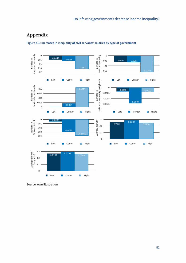
Do left-wing governments decrease income inequality?
81
Appendix
Figure 4.1: Increases in inequality of civil servants’ salaries by type of government
Source: own illustration.
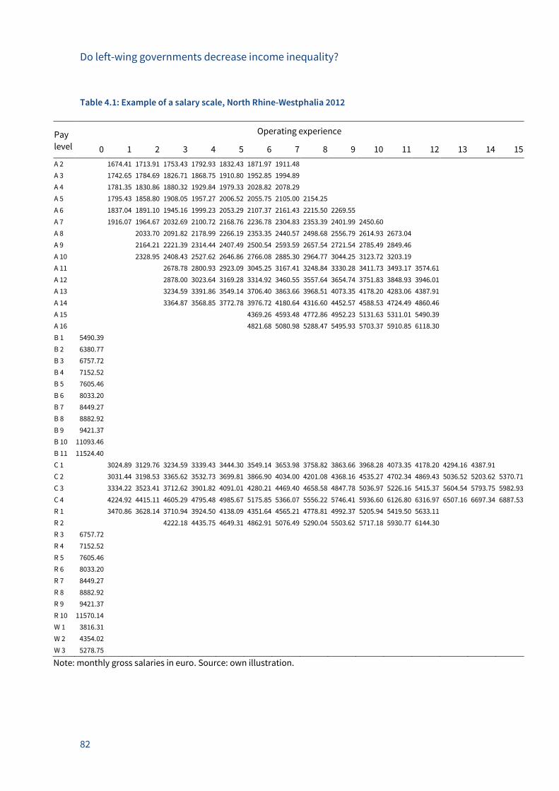
Do left-wing governments decrease income inequality?
82
Table 4.1: Example of a salary scale, North Rhine-Westphalia 2012
Pay
level
Operating experience
0 1 2 3 4 5 6 7 8 9 10 11 12 13 14 15
A 2 1674.41 1713.91 1753.43 1792.93 1832.43 1871.97 1911.48 A 3 1742.65 1784.69 1826.71 1868.75 1910.80 1952.85 1994.89 A 4 1781.35 1830.86 1880.32 1929.84 1979.33 2028.82 2078.29 A 5 1795.43 1858.80 1908.05 1957.27 2006.52 2055.75 2105.00 2154.25 A 6 1837.04 1891.10 1945.16 1999.23 2053.29 2107.37 2161.43 2215.50 2269.55 A 7 1916.07 1964.67 2032.69 2100.72 2168.76 2236.78 2304.83 2353.39 2401.99 2450.60 A 8 2033.70 2091.82 2178.99 2266.19 2353.35 2440.57 2498.68 2556.79 2614.93 2673.04 A 9 2164.21 2221.39 2314.44 2407.49 2500.54 2593.59 2657.54 2721.54 2785.49 2849.46 A 10 2328.95 2408.43 2527.62 2646.86 2766.08 2885.30 2964.77 3044.25 3123.72 3203.19 A 11 2678.78 2800.93 2923.09 3045.25 3167.41 3248.84 3330.28 3411.73 3493.17 3574.61 A 12 2878.00 3023.64 3169.28 3314.92 3460.55 3557.64 3654.74 3751.83 3848.93 3946.01 A 13 3234.59 3391.86 3549.14 3706.40 3863.66 3968.51 4073.35 4178.20 4283.06 4387.91 A 14 3364.87 3568.85 3772.78 3976.72 4180.64 4316.60 4452.57 4588.53 4724.49 4860.46 A 15 4369.26 4593.48 4772.86 4952.23 5131.63 5311.01 5490.39 A 16 4821.68 5080.98 5288.47 5495.93 5703.37 5910.85 6118.30 B 1 5490.39 B 2 6380.77 B 3 6757.72 B 4 7152.52 B 5 7605.46 B 6 8033.20 B 7 8449.27 B 8 8882.92 B 9 9421.37 B 10 11093.46 B 11 11524.40 C 1 3024.89 3129.76 3234.59 3339.43 3444.30 3549.14 3653.98 3758.82 3863.66 3968.28 4073.35 4178.20 4294.16 4387.91 C 2 3031.44 3198.53 3365.62 3532.73 3699.81 3866.90 4034.00 4201.08 4368.16 4535.27 4702.34 4869.43 5036.52 5203.62 5370.71
C 3 3334.22 3523.41 3712.62 3901.82 4091.01 4280.21 4469.40 4658.58 4847.78 5036.97 5226.16 5415.37 5604.54 5793.75 5982.93
C 4 4224.92 4415.11 4605.29 4795.48 4985.67 5175.85 5366.07 5556.22 5746.41 5936.60 6126.80 6316.97 6507.16 6697.34 6887.53
R 1 3470.86 3628.14 3710.94 3924.50 4138.09 4351.64 4565.21 4778.81 4992.37 5205.94 5419.50 5633.11 R 2 4222.18 4435.75 4649.31 4862.91 5076.49 5290.04 5503.62 5717.18 5930.77 6144.30 R 3 6757.72 R 4 7152.52 R 5 7605.46 R 6 8033.20 R 7 8449.27 R 8 8882.92 R 9 9421.37 R 10 11570.14 W 1 3816.31 W 2 4354.02 W 3 5278.75
Note: monthly gross salaries in euro. Source: own illustration.
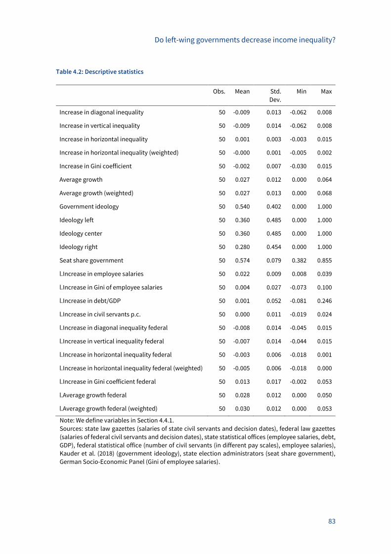
Do left-wing governments decrease income inequality?
83
Table 4.2: Descriptive statistics
Obs. Mean Std.
Dev.
Min Max
Increase in diagonal inequality 50 -0.009 0.013 -0.062 0.008
Increase in vertical inequality 50 -0.009 0.014 -0.062 0.008
Increase in horizontal inequality 50 0.001 0.003 -0.003 0.015
Increase in horizontal inequality (weighted) 50 -0.000 0.001 -0.005 0.002
Increase in Gini coefficient 50 -0.002 0.007 -0.030 0.015
Average growth 50 0.027 0.012 0.000 0.064
Average growth (weighted) 50 0.027 0.013 0.000 0.068
Government ideology 50 0.540 0.402 0.000 1.000
Ideology left 50 0.360 0.485 0.000 1.000
Ideology center 50 0.360 0.485 0.000 1.000
Ideology right 50 0.280 0.454 0.000 1.000
Seat share government 50 0.574 0.079 0.382 0.855
l.Increase in employee salaries 50 0.022 0.009 0.008 0.039
l.Increase in Gini of employee salaries 50 0.004 0.027 -0.073 0.100
l.Increase in debt/GDP 50 0.001 0.052 -0.081 0.246
l.Increase in civil servants p.c. 50 0.000 0.011 -0.019 0.024
l.Increase in diagonal inequality federal 50 -0.008 0.014 -0.045 0.015
l.Increase in vertical inequality federal 50 -0.007 0.014 -0.044 0.015
l.Increase in horizontal inequality federal 50 -0.003 0.006 -0.018 0.001
l.Increase in horizontal inequality federal (weighted) 50 -0.005 0.006 -0.018 0.000
l.Increase in Gini coefficient federal 50 0.013 0.017 -0.002 0.053
l.Average growth federal 50 0.028 0.012 0.000 0.050
l.Average growth federal (weighted) 50 0.030 0.012 0.000 0.053
Note: We define variables in Section 4.4.1.
Sources: state law gazettes (salaries of state civil servants and decision dates), federal law gazettes
(salaries of federal civil servants and decision dates), state statistical offices (employee salaries, debt,
GDP), federal statistical office (number of civil servants (in different pay scales), employee salaries),
Kauder et al. (2018) (government ideology), state election administrators (seat share government),
German Socio-Economic Panel (Gini of employee salaries).
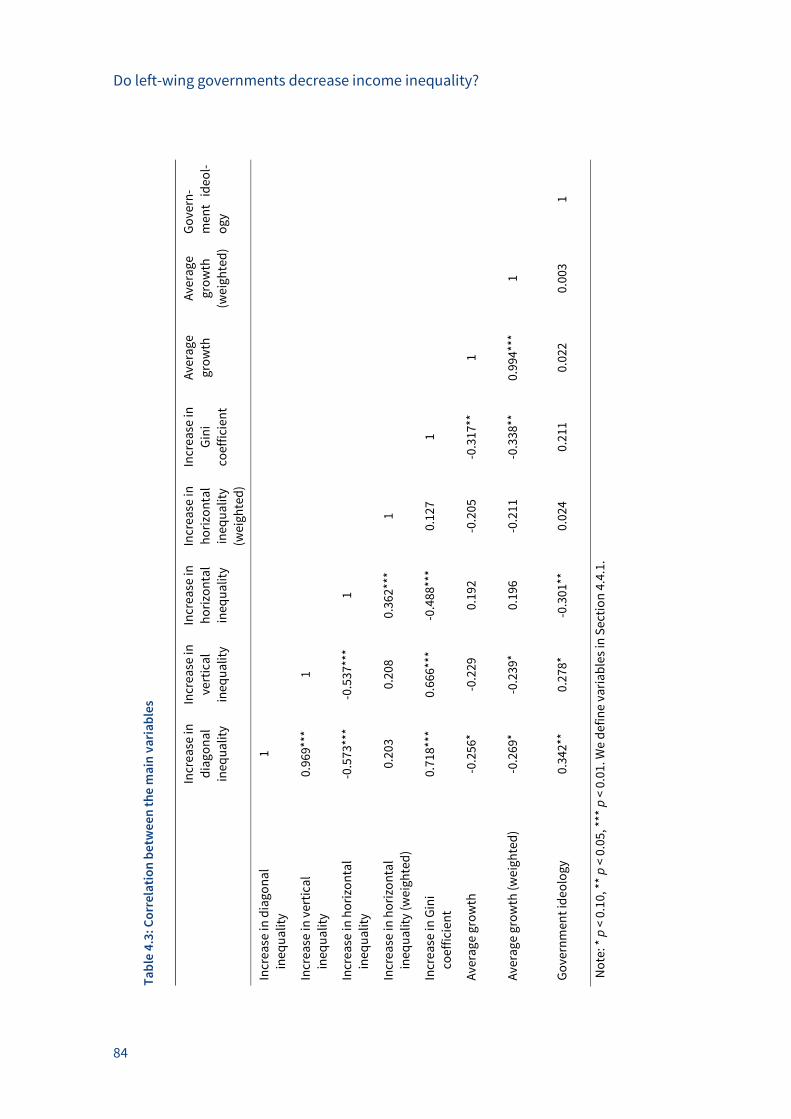
Do left-wing governments decrease income inequality?
84
Ta
ble
4.3
: Co
rre
lati
on
be
twe
en
th
e m
ain
va
ria
ble
s
In
crea
se in
dia
go
na
l
ineq
ua
lity
Incr
ease
in
vert
ica
l
ineq
ua
lity
Incr
ease
in
ho
rizo
nta
l
ineq
ua
lity
Incr
ease
in
ho
rizo
nta
l
ineq
ua
lity
(wei
gh
ted
)
Incr
ease
in
Gin
i
coef
fici
ent
Ave
rag
e
gro
wth
Ave
rag
e
gro
wth
(wei
gh
ted
)
Go
vern
-
men
t id
eo
l-
og
y
Incr
ease
in d
iag
on
al
ineq
ua
lity
1
Incr
ease
in v
erti
cal
ineq
ua
lity
0.96
9***
1
Incr
ease
in h
ori
zon
tal
ineq
ua
lity
-0.5
73**
* -0
.537
***
1
Incr
ease
in h
ori
zon
tal
ineq
ua
lity
(we
igh
ted
)
0.20
3
0.20
8
0.36
2***
1
Incr
ease
in G
ini
coef
fici
ent
0.71
8***
0.
666*
**
-0.4
88**
* 0.
127
1
Ave
rag
e g
row
th
-0.2
56*
-0.2
29
0.19
2
-0.2
05
-0.3
17**
1
Ave
rag
e g
row
th (
we
igh
ted
) -0
.269
* -0
.239
* 0.
196
-0
.211
-0
.338
**
0.99
4***
1
Go
vern
men
t id
eo
log
y
0.34
2**
0.27
8*
-0.3
01**
0.
024
0.
211
0.
022
0.
003
1
No
te: *
p <
0.1
0, *
* p
< 0
.05,
***
p <
0.0
1. W
e d
efi
ne
vari
ab
les
in S
ecti
on
4.4
.1.
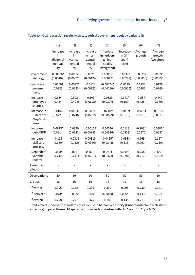
Do left-wing governments decrease income inequality?
85
Table 4.4: OLS regression results with categorical government ideology variable (I)
(1) (2) (3) (4) (5) (6) (7)
Increase
in
diagonal
inequal-
ity
Increase
in
vertical
inequal-
ity
Increase
in hori-
zontal
inequal-
ity
Increase
in horizon-
tal ine-
quality
(weighted)
Increase
in Gini
coeffi-
cient
Average
growth
Average
growth
(weighted)
Government
ideology
0.00906* 0.00855 -0.00216 0.000557 0.00393 0.00797 0.00598
(0.00467) (0.00528) (0.00124) (0.000471) (0.00291) (0.00856) (0.00855)
Seat share
govern-
ment
0.00501 0.00926 -0.0128 -0.00574* -0.0119 0.0138 0.0129
(0.0223) (0.0223) (0.00922) (0.00290) (0.00929) (0.0286) (0.0260)
l.Increase in
employee
salaries
0.664 0.602 -0.109 -0.0529 0.341* -0.587 -0.442
(0.434) (0.494) (0.0698) (0.0307) (0.169) (0.425) (0.380)
l.Increase in
Gini of em-
ployee sal-
aries
0.0166 0.00830 0.0415* 0.0238** -0.0489 -0.0293 -0.0109
(0.0729) (0.0746) (0.0202) (0.00829) (0.0516) (0.0913) (0.0811)
l.Increase in
debt/GDP
0.0913* 0.0820 -0.00153 0.00540 0.0113 -0.108* -0.0986*
(0.0514) (0.0523) (0.00843) (0.00526) (0.0233) (0.0570) (0.0537)
l.Increase in
civil serv-
ants p.c.
-0.139 -0.0319 0.00315 -0.0465* -0.0938 0.169 0.157
(0.120) (0.112) (0.0386) (0.0243) (0.115) (0.291) (0.256)
l.Dependent
variable
federal
0.0384 0.0261 0.168* 0.0434 0.0996 0.258 0.400*
(0.242) (0.271) (0.0791) (0.0323) (0.0784) (0.217) (0.192)
Time-fixed
effects
- - - - - - -
Observations 50 50 50 50 50 50 50
Groups 16 16 16 16 16 16 16
R² within 0.395 0.332 0.366 0.392 0.298 0.230 0.321
R² between 0.0734 0.0372 0.420 0.00858 0.00546 0.143 0.304
R² overall 0.298 0.227 0.375 0.189 0.135 0.211 0.317
Fixed-effects model with standard errors robust to heteroskedasticity (Huber/White/sandwich stand-
ard errors) in parentheses. All specifications include state-fixed effects. * p < 0.10, ** p < 0.05.
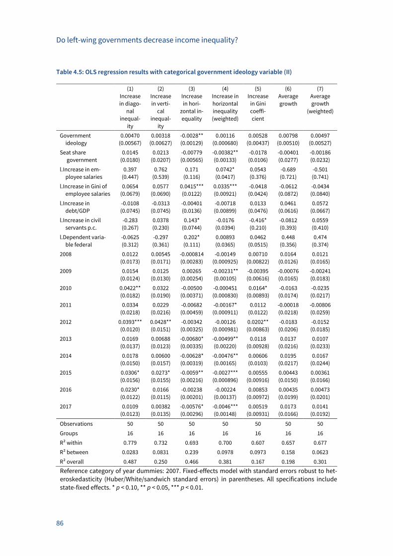
Do left-wing governments decrease income inequality?
86
Table 4.5: OLS regression results with categorical government ideology variable (II)
(1) (2) (3) (4) (5) (6) (7)
Increase
in diago-
nal
inequal-
ity
Increase
in verti-
cal
inequal-
ity
Increase
in hori-
zontal in-
equality
Increase in
horizontal
inequality
(weighted)
Increase
in Gini
coeffi-
cient
Average
growth
Average
growth
(weighted)
Government
ideology
0.00470 0.00318 -0.0028** 0.00116 0.00528 0.00798 0.00497
(0.00567) (0.00627) (0.00129) (0.000680) (0.00437) (0.00510) (0.00527)
Seat share
government
0.0145 0.0213 -0.00779 -0.00382** -0.0178 -0.00401 -0.00186
(0.0180) (0.0207) (0.00565) (0.00133) (0.0106) (0.0277) (0.0232)
l.Increase in em-
ployee salaries
0.397 0.762 0.171 0.0742* 0.0543 -0.689 -0.501
(0.447) (0.539) (0.116) (0.0417) (0.376) (0.721) (0.741)
l.Increase in Gini of
employee salaries
0.0654 0.0577 0.0415*** 0.0335*** -0.0418 -0.0612 -0.0434
(0.0679) (0.0690) (0.0122) (0.00921) (0.0424) (0.0872) (0.0840)
l.Increase in
debt/GDP
-0.0108 -0.0313 -0.00401 -0.00718 0.0133 0.0461 0.0572
(0.0745) (0.0745) (0.0136) (0.00899) (0.0476) (0.0616) (0.0667)
l.Increase in civil
servants p.c.
-0.283 0.0378 0.143* -0.0176 -0.416* -0.0812 0.0559
(0.267) (0.230) (0.0744) (0.0394) (0.210) (0.393) (0.410)
l.Dependent varia-
ble federal
-0.0625 -0.297 0.202* 0.00893 0.0462 0.448 0.474
(0.312) (0.361) (0.111) (0.0365) (0.0515) (0.356) (0.374)
2008 0.0122 0.00545 -0.000814 -0.00149 0.00710 0.0164 0.0121
(0.0173) (0.0171) (0.00283) (0.000925) (0.00822) (0.0126) (0.0165)
2009 0.0154 0.0125 0.00265 -0.00231** -0.00395 -0.00076 -0.00241
(0.0124) (0.0130) (0.00254) (0.00105) (0.00616) (0.0165) (0.0183)
2010 0.0422** 0.0322 -0.00500 -0.000451 0.0164* -0.0163 -0.0235
(0.0182) (0.0190) (0.00371) (0.000830) (0.00893) (0.0174) (0.0217)
2011 0.0334 0.0229 -0.00682 -0.00167* 0.0112 -0.00018 -0.00806
(0.0218) (0.0216) (0.00459) (0.000911) (0.0122) (0.0218) (0.0259)
2012 0.0393*** 0.0428** -0.00342 -0.00126 0.0202** -0.0183 -0.0152
(0.0120) (0.0151) (0.00325) (0.000981) (0.00863) (0.0206) (0.0185)
2013 0.0169 0.00688 -0.00680* -0.00499** 0.0118 0.0137 0.0107
(0.0137) (0.0123) (0.00335) (0.00220) (0.00928) (0.0216) (0.0233)
2014 0.0178 0.00600 -0.00628* -0.00476** 0.00606 0.0195 0.0167
(0.0150) (0.0157) (0.00319) (0.00165) (0.0103) (0.0217) (0.0244)
2015 0.0306* 0.0273* -0.0059** -0.0027*** 0.00555 0.00443 0.00361
(0.0156) (0.0155) (0.00216) (0.000896) (0.00916) (0.0150) (0.0166)
2016 0.0230* 0.0166 -0.00238 -0.00224 0.00853 0.00435 0.00473
(0.0122) (0.0115) (0.00201) (0.00137) (0.00972) (0.0199) (0.0201)
2017 0.0109 0.00382 -0.00576* -0.0046*** 0.00519 0.0173 0.0141
(0.0123) (0.0135) (0.00296) (0.00148) (0.00931) (0.0166) (0.0192)
Observations 50 50 50 50 50 50 50
Groups 16 16 16 16 16 16 16
R² within 0.779 0.732 0.693 0.700 0.607 0.657 0.677
R² between 0.0283 0.0831 0.239 0.0978 0.0973 0.158 0.0623
R² overall 0.487 0.250 0.466 0.381 0.167 0.198 0.301
Reference category of year dummies: 2007. Fixed-effects model with standard errors robust to het-
eroskedasticity (Huber/White/sandwich standard errors) in parentheses. All specifications include
state-fixed effects. * p < 0.10, ** p < 0.05, *** p < 0.01.
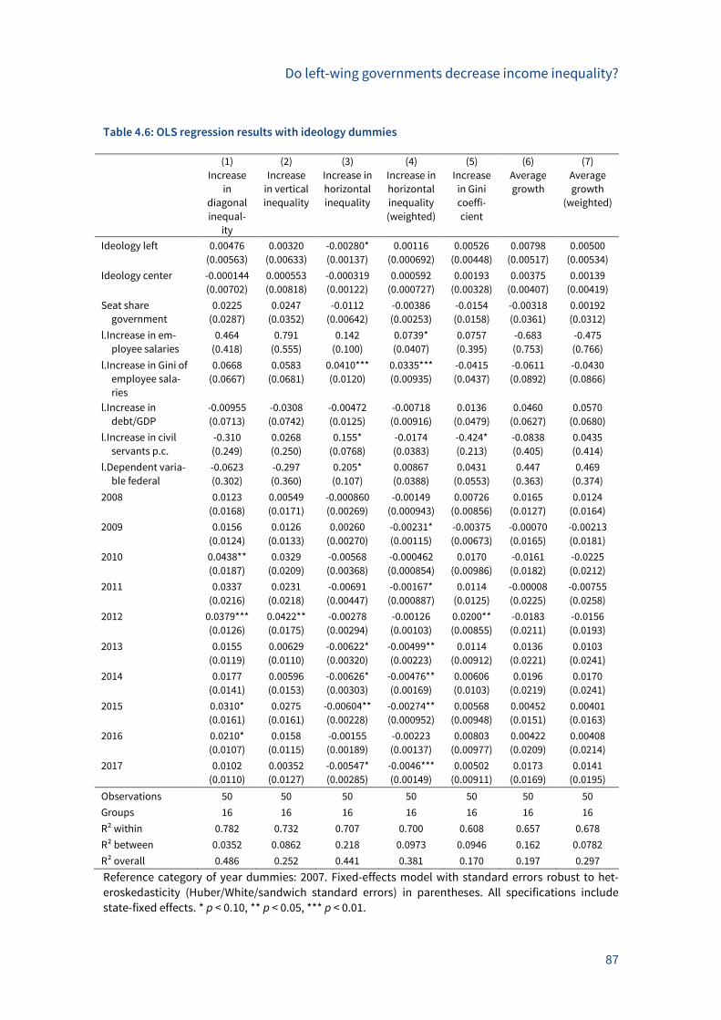
Do left-wing governments decrease income inequality?
87
Table 4.6: OLS regression results with ideology dummies
(1) (2) (3) (4) (5) (6) (7)
Increase
in
diagonal
inequal-
ity
Increase
in vertical
inequality
Increase in
horizontal
inequality
Increase in
horizontal
inequality
(weighted)
Increase
in Gini
coeffi-
cient
Average
growth
Average
growth
(weighted)
Ideology left 0.00476 0.00320 -0.00280* 0.00116 0.00526 0.00798 0.00500
(0.00563) (0.00633) (0.00137) (0.000692) (0.00448) (0.00517) (0.00534)
Ideology center -0.000144 0.000553 -0.000319 0.000592 0.00193 0.00375 0.00139
(0.00702) (0.00818) (0.00122) (0.000727) (0.00328) (0.00407) (0.00419)
Seat share
government
0.0225 0.0247 -0.0112 -0.00386 -0.0154 -0.00318 0.00192
(0.0287) (0.0352) (0.00642) (0.00253) (0.0158) (0.0361) (0.0312)
l.Increase in em-
ployee salaries
0.464 0.791 0.142 0.0739* 0.0757 -0.683 -0.475
(0.418) (0.555) (0.100) (0.0407) (0.395) (0.753) (0.766)
l.Increase in Gini of
employee sala-
ries
0.0668 0.0583 0.0410*** 0.0335*** -0.0415 -0.0611 -0.0430
(0.0667) (0.0681) (0.0120) (0.00935) (0.0437) (0.0892) (0.0866)
l.Increase in
debt/GDP
-0.00955 -0.0308 -0.00472 -0.00718 0.0136 0.0460 0.0570
(0.0713) (0.0742) (0.0125) (0.00916) (0.0479) (0.0627) (0.0680)
l.Increase in civil
servants p.c.
-0.310 0.0268 0.155* -0.0174 -0.424* -0.0838 0.0435
(0.249) (0.250) (0.0768) (0.0383) (0.213) (0.405) (0.414)
l.Dependent varia-
ble federal
-0.0623 -0.297 0.205* 0.00867 0.0431 0.447 0.469
(0.302) (0.360) (0.107) (0.0388) (0.0553) (0.363) (0.374)
2008 0.0123 0.00549 -0.000860 -0.00149 0.00726 0.0165 0.0124
(0.0168) (0.0171) (0.00269) (0.000943) (0.00856) (0.0127) (0.0164)
2009 0.0156 0.0126 0.00260 -0.00231* -0.00375 -0.00070 -0.00213
(0.0124) (0.0133) (0.00270) (0.00115) (0.00673) (0.0165) (0.0181)
2010 0.0438** 0.0329 -0.00568 -0.000462 0.0170 -0.0161 -0.0225
(0.0187) (0.0209) (0.00368) (0.000854) (0.00986) (0.0182) (0.0212)
2011 0.0337 0.0231 -0.00691 -0.00167* 0.0114 -0.00008 -0.00755
(0.0216) (0.0218) (0.00447) (0.000887) (0.0125) (0.0225) (0.0258)
2012 0.0379*** 0.0422** -0.00278 -0.00126 0.0200** -0.0183 -0.0156
(0.0126) (0.0175) (0.00294) (0.00103) (0.00855) (0.0211) (0.0193)
2013 0.0155 0.00629 -0.00622* -0.00499** 0.0114 0.0136 0.0103
(0.0119) (0.0110) (0.00320) (0.00223) (0.00912) (0.0221) (0.0241)
2014 0.0177 0.00596 -0.00626* -0.00476** 0.00606 0.0196 0.0170
(0.0141) (0.0153) (0.00303) (0.00169) (0.0103) (0.0219) (0.0241)
2015 0.0310* 0.0275 -0.00604** -0.00274** 0.00568 0.00452 0.00401
(0.0161) (0.0161) (0.00228) (0.000952) (0.00948) (0.0151) (0.0163)
2016 0.0210* 0.0158 -0.00155 -0.00223 0.00803 0.00422 0.00408
(0.0107) (0.0115) (0.00189) (0.00137) (0.00977) (0.0209) (0.0214)
2017 0.0102 0.00352 -0.00547* -0.0046*** 0.00502 0.0173 0.0141
(0.0110) (0.0127) (0.00285) (0.00149) (0.00911) (0.0169) (0.0195)
Observations 50 50 50 50 50 50 50
Groups 16 16 16 16 16 16 16
R² within 0.782 0.732 0.707 0.700 0.608 0.657 0.678
R² between 0.0352 0.0862 0.218 0.0973 0.0946 0.162 0.0782
R² overall 0.486 0.252 0.441 0.381 0.170 0.197 0.297
Reference category of year dummies: 2007. Fixed-effects model with standard errors robust to het-
eroskedasticity (Huber/White/sandwich standard errors) in parentheses. All specifications include
state-fixed effects. * p < 0.10, ** p < 0.05, *** p < 0.01.
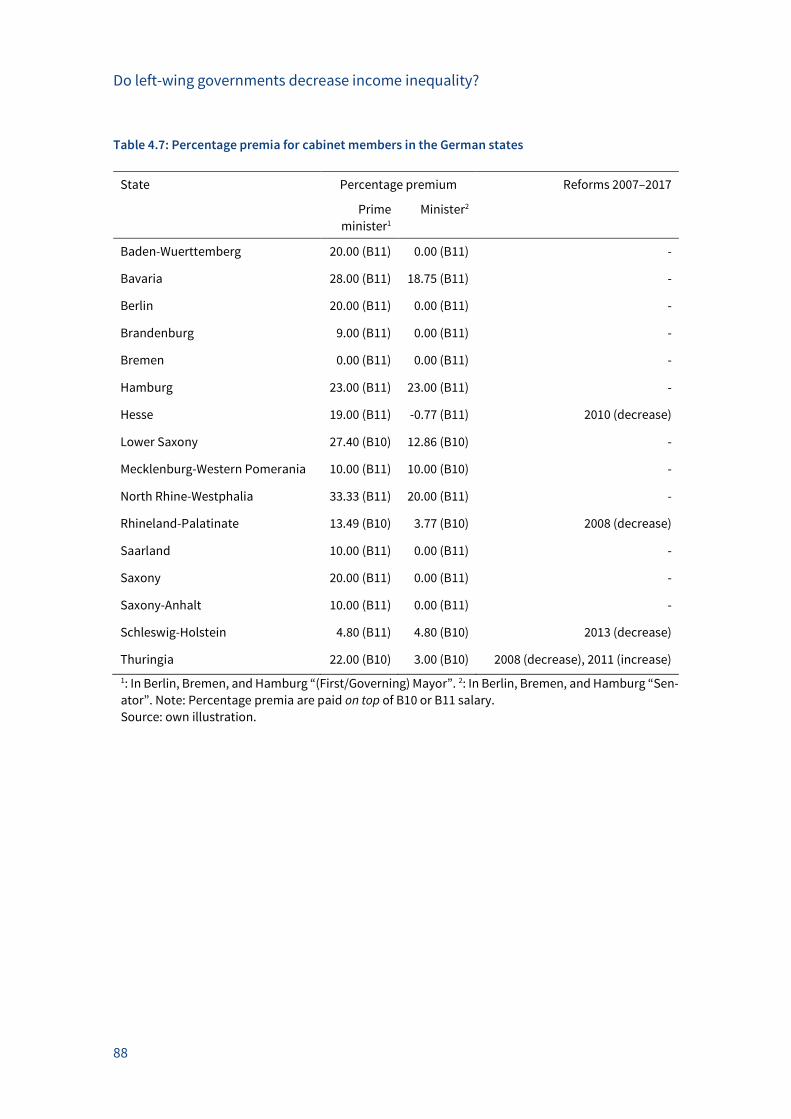
Do left-wing governments decrease income inequality?
88
Table 4.7: Percentage premia for cabinet members in the German states
State Percentage premium Reforms 2007–2017
Prime
minister1
Minister2
Baden-Wuerttemberg 20.00 (B11) 0.00 (B11) -
Bavaria 28.00 (B11) 18.75 (B11) -
Berlin 20.00 (B11) 0.00 (B11) -
Brandenburg 9.00 (B11) 0.00 (B11) -
Bremen 0.00 (B11) 0.00 (B11) -
Hamburg 23.00 (B11) 23.00 (B11) -
Hesse 19.00 (B11) -0.77 (B11) 2010 (decrease)
Lower Saxony 27.40 (B10) 12.86 (B10) -
Mecklenburg-Western Pomerania 10.00 (B11) 10.00 (B10) -
North Rhine-Westphalia 33.33 (B11) 20.00 (B11) -
Rhineland-Palatinate 13.49 (B10) 3.77 (B10) 2008 (decrease)
Saarland 10.00 (B11) 0.00 (B11) -
Saxony 20.00 (B11) 0.00 (B11) -
Saxony-Anhalt 10.00 (B11) 0.00 (B11) -
Schleswig-Holstein 4.80 (B11) 4.80 (B10) 2013 (decrease)
Thuringia 22.00 (B10) 3.00 (B10) 2008 (decrease), 2011 (increase)
1: In Berlin, Bremen, and Hamburg “(First/Governing) Mayor”. 2: In Berlin, Bremen, and Hamburg “Sen-
ator”. Note: Percentage premia are paid on top of B10 or B11 salary.
Source: own illustration.
The real-estate transfer tax and government ideology
89
5 The real-estate transfer tax
and government ideology:
Evidence from the German states
The real-estate transfer tax and government ideology
Abstract*
In 2006, the reform of the German fiscal constitution realigned legislative powers between the
federal and the state governments. The reform allowed German state governments to set the
real-estate transfer tax rates – an important reform because German state governments have
had basically no authority to set tax policies before. We investigate whether government ide-
ology predicts the levels and increases in the real-estate transfer tax rates. The results show
that left-wing and center governments were more active in increasing the real-estate transfer
tax rates than right-wing governments. Many voters were disenchanted with the policies and
platforms of the established German parties in the course of the euro and refugee crisis. Dis-
enchantment notwithstanding, real-estate transfer tax policies show that the established po-
litical parties are still prepared to offer polarized policies.
* This chapter is based on joint work with Niklas Potrafke. It is based on our paper “The real-estate transfer tax and government
ideology: Evidence from the German states”, CESifo Working Paper 6491, 2017. We thank Thiess Büttner, Julie Cullen, Gordon Dahl, Marc Debus, Björn Kauder, Markus Tepe and participants of the Annual Conference of the Canadian Economic Association
for helpful comments and Lisa Giani Contini for proof-reading. Roman Klimke and Antonia Kremheller provided excellent re-
search assistance.
The real-estate transfer tax and government ideology
90
Introduction
Partisan theories hold that government ideology influences economic policy-making: left-
wing governments are expected to implement more expansionary economic policies than
right-wing governments (Hibbs 1977, Chappell and Keech 1986, Alesina 1987), and as a result,
the size and scope of government is larger under left-wing than right-wing governments. A
large size and scope of government includes, for example, pronounced public expenditure,
taxes, debt and regulation of labor and product markets. Partisan politicians gratify the needs
of their constituencies. Left-wing politicians are inclined to gratify the needs of low-income
citizens (the working class), while right-wing politicians are inclined to gratify the needs of
high-income citizens (traditionally the self-employed). Partisan politicians are therefore also
expected not just to increase or decrease the size and scope of government; they will also
design individual policy measures such as taxes to reward their constituencies. For example,
left-wing governments are likely to tax capital to a larger extent than labor.
Many empirical studies have examined whether government ideology predicts individual eco-
nomic policies (for new studies see, for example, Jäger 2017 and Schmitt and Zohlnhöfer
2018). Scholars use panel data for OECD countries and for states within federal countries, uni-
variate time series for individual countries, as well as data for municipalities in particular, to
derive causal effects (by employing, for example, Regression Discontinuity Designs – RDD – for
close vote margins between left-wing and right-wing politicians). The evidence is mixed as to
whether parties influence economic policy-making. For comprehensive surveys on partisan
politics, see Potrafke (2017 and 2018) and Zohlnhöfer et al. (2018).
Investigating whether parties matter in economic policy-making is important because in
many industrialized countries, the platforms and (individual) policies of established parties
have converged since the 1990s. It is conceivable that many voters are disenchanted with the
policies of the established parties, desire more polarized policies, and in turn, have started to
support new parties entering the political arena. Examples include the populist left-wing
SYRIZA in Greece (in the 2000s the social democratic PASOK and the conservative New Democ-
racy won a combined total of around 80 percent of the votes, while in 2015 PASOK and New
Democracy won a combined total of just 30 percent of the votes) and the populist right-wing
Freedom Party in Austria (the Freedom Party was founded many decades ago, but has won
significant electoral support since the 1990s).
Another example is Germany. When he took office in 2002 (his second term) the then chancel-
lor Gerhard Schröder moved his Social Democratic Party (SPD) towards the middle of the po-
litical spectrum. His coalition government with the Greens implemented some fairly market-
oriented policies such as liberalizing the labor market. As a result, the populist left-wing party
DIE LINKE entered the political arena. Since the mid-2000s, the voting share of the left-wing
SPD has decreased in federal elections (see, for example, Debus 2008). The right-wing Chris-
tian Conservative Union (CDU) moved towards the middle of the political spectrum when it
The real-estate transfer tax and government ideology
91
formed a grand coalition with the SPD in 2005. Economic policy positions in particular became
far less market-oriented than at the beginning of the 2000s. Bailout policies in the course of
the euro crisis diluted the economic policy platform of the CDU. A new populist right-wing
party, the Alternative for Germany, was successful in many German state elections in 2015 and
2016. In the course of the refugee crisis in 2015, the CDU pursued a liberal immigration policy
– alienating many core conservative voters. A precondition for the electoral success of the SPD
and the CDU would seem to be more polarized policies.
There have been studies showing that the SPD and the CDU, being part of left-wing and right-
wing governments, pursued different policies in the German states. For instance, right-wing
governments spent more on universities and cultural affairs, were more active in introducing
tuition fees, hired more policemen, and promoted greater economic freedom than left-wing
governments (Oberndorfer and Steiner 2007, Potrafke 2011, Kauder and Potrafke 2013, Tepe
and Vanhuysse 2013, Potrafke 2013). By contrast, public debt policies hardly differed between
left-wing and right-wing state governments (Jochimsen and Nuscheler 2011, Jochimsen and
Thomasius 2014, Potrafke et al. 2016).1 Experts have not yet examined ideology-induced tax
policies in the German states. The reason is that German state governments have had basi-
cally no authority to set tax policies.2 Empirical tests of ideology-induced policies in the Ger-
man states require, of course, examining policies that are influenced by the state govern-
ments (and not determined by the federal government).
In the course of the reform of the German fiscal constitution in 2006, the allocation of rights
and duties between the federal and the state governments was realigned.3 German state gov-
ernments were allowed to set the real-estate transfer tax rates. The real-estate transfer tax
thus became after a long time the first tax for which the state governments have the authority
to set the tax rates.4 Some state governments began to increase the real-estate transfer tax
rate immediately in 2007. Other states have not increased the tax rate ever since. Allowing the
German state governments to determine the real-estate transfer tax rates provides an excel-
lent laboratory for investigating the prediction of partisan theories.
1 On ideology-induced policies at the local level see, for example, Roesel (2017).
2 See Herwartz and Theilen (2014) for the extent to which state government ideology predicted efforts to collect tax revenues (for
taxes set at the federal level). Koester (2009) investigates determinants of the tax policy on the federal level. While normative approaches are mostly unable to explain tax reforms, political economic reasons influence tax policy on the federal level. How-
ever, the author does not find evidence for ideology-induced tax policies at the federal level.
3 Hildebrandt (2016) portrays the implications of the federalism reforms on the state fiscal policies.
4 Scholars investigate the economic consequences of the real-estate transfer tax in Germany. Buettner (2017) examines welfare
effects of the real-estate transfer tax. Buettner and Krause (2018a, b) examine the extent to which the fiscal equalization scheme
affects states’ tax policy (see also Chapters 6 and 7). Fritzsche and Vandrei (2016) investigate how the real-estate transfer tax
influences the number of real-estate transactions in Germany. Petkova and Weichenrieder (2017) investigate the effect of the
real-estate transfer tax on prices of single-family houses and apartments.
The real-estate transfer tax and government ideology
92
The real-estate transfer tax is likely to influence citizens who own property – usually high-in-
come citizens – and therefore seems suitable for redistributing income from the rich to the
poor. Right-wing politicians are generally more hesitant to increase tax rates and view the
purchase of real estate as worthy of support.5 Left-wing politicians, by contrast, are more in
favor of income redistribution. The hypotheses to be tested empirically are: left-wing govern-
ments are more active in increasing real-estate transfer tax rates than right-wing govern-
ments, and as a result, real-estate transfer tax rates are higher under left-wing than right-wing
governments. We examine these hypotheses by case study evidence and descriptive statistics.
We use state-year data for the 16 German states over the period 2007–2017. As we could not
overcome the potential endogeneity of the government ideology variable when regressing
real-estate transfer tax rates on government ideology (we cannot rule out reverse causality or
that there is a third unobserved variable influencing both real-estate transfer tax rates and
government ideology), we cannot estimate causal effects but elaborate on correlations. More-
over, the sample is too small to exploit close vote margins and use, for example, an RDD.
Institutional background
5.2.1 State governments in Germany’s federalism
In Germany, the federal structure defines different rights and duties for the federal level, the
states and the municipalities. In general, the state governments are responsible for dealing
with the tasks of the states (including legislation) and executing the laws. The states are
mostly also responsible for the financing of these tasks because the administrative and finan-
cial responsibility are linked according to the constitution. In any event, in some specific
cases, the federal government helps the state governments to finance interests of the states.
To fulfill the financial responsibilities, the state governments have different revenue sources.
The main part of the states’ tax revenues are shared taxes. Those taxes cover over three quar-
ters of overall states’ tax revenues. Revenues of the shared taxes include the revenues of the
value added tax (VAT), the income tax, and the corporate tax and are shared among the fed-
eral, state and local governments. The states also obtain revenues from state taxes, whose
amounts are exclusively for the states. The real-estate transfer tax is part of the state taxes.
Moreover, a fiscal equalization scheme with horizontal and vertical stages redistributes reve-
nues among the different levels and between the states. For a long time, the states had basi-
cally no means to determine the rates of any tax. In 2006, a reform of the German fiscal con-
stitution realigned legislative powers between the federal and the state governments. The
reform aimed to improve the efficiency within the federal system and to deconcentrate finan-
cial responsibilities between the federal level and the states. The reform also strengthened
the tax autonomy of the state level by allowing the states to set the tax rate of the real-estate
5 Studies on ideology-induced tax policies include Quinn and Shapiro (1991), Beramendi and Cusack (2006), Beramendi and
Rueda (2007), Angelopoulos et al. (2012), Osterloh and Debus (2012).
The real-estate transfer tax and government ideology
93
transfer tax. In general, federal law determines the tax bases and tax rates of the most im-
portant taxes – the real-estate transfer tax being the first exception.
5.2.2 The German real-estate transfer tax
The German real-estate transfer tax has to be paid on the price of the real estate determined
in the contract between the selling and the purchasing party. The German real-estate transfer
tax law describes that both seller and buyer are held responsible for the liability of the tax.
The amount of tax will be transferred to the authorities by the contracting party that has been
declared the taxpayer in the contract, which is usually the buyer of the real estate. Purchases
of less than 2,500 euro or real-estate transfers due to inheritance or donation are exempt from
the tax.
Since 2007, 14 out of the 16 states have increased real-estate transfer tax rates to levels of up
to 6.5 percent (Brandenburg, North Rhine-Westphalia, Saarland, Schleswig-Holstein, Thurin-
gia). Bavaria and Saxony are the only two states where the tax rate has remained at its pre-
reform level of 3.5 percent. The real-estate transfer tax revenue collected by the federal states
has risen from 4.8 in 2005 to 13.14 billion euro in 2017, amounting to an increase of 174 per-
cent according to the Federal Ministry of Finance. In 2017, the real-estate transfer tax was the
most important state tax. The share of the real-estate transfer tax with regard to the overall
state taxes, whose amounts are exclusively for the states, was 59.2 percent. However, the real-
estate transfer tax amounts to only 4.4 percent of the total amount of taxes received by federal
states, which includes the shared taxes and also transfers from the German federal govern-
ment to the states.
Comparing real-estate transfer taxes internationally remains difficult, because the laws of tax
exemption and the taxable bases differ across countries. For example, in contrast to Germany,
some countries set real-estate transfer tax rates on constituent real estate, while newly-built
real estate applies to the value-added taxation. Moreover, in Germany, the tax base is taxed
by a fixed rate differing across states. In Australia and Cyprus, for example, the real-estate
transfer tax rate increases progressively with the value of the real estate and is determined at
the national level. In any event, real-estate transfers tax rates are fairly high in Germany com-
pared to other countries (Bechtoldt et al. 2014).
Case study evidence
Table 5.1 shows the real-estate transfer tax rates and the ideology of the government imple-
menting tax increases in the individual states. In Baden-Wuerttemberg, there was a right-wing
government for many decades (a grand coalition over the period 1992–1996 being an excep-
tion). In spring 2011, however, a left-wing Green-SPD government came into power which in-
creased the real-estate transfer tax rate from 3.5 percent to 5 percent as of 5 November 2011.
In Bavaria, there has been a right-wing government since the 1950s. Bavaria is one of the two
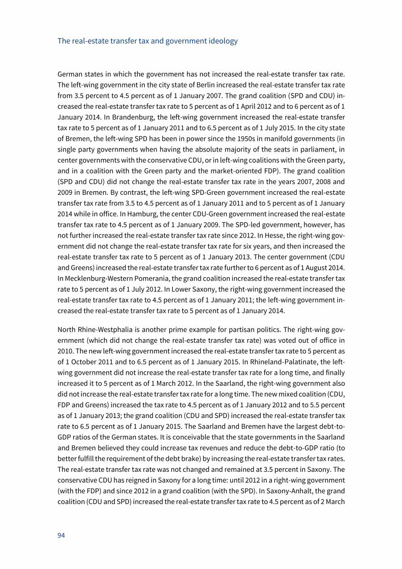
The real-estate transfer tax and government ideology
94
German states in which the government has not increased the real-estate transfer tax rate.
The left-wing government in the city state of Berlin increased the real-estate transfer tax rate
from 3.5 percent to 4.5 percent as of 1 January 2007. The grand coalition (SPD and CDU) in-
creased the real-estate transfer tax rate to 5 percent as of 1 April 2012 and to 6 percent as of 1
January 2014. In Brandenburg, the left-wing government increased the real-estate transfer
tax rate to 5 percent as of 1 January 2011 and to 6.5 percent as of 1 July 2015. In the city state
of Bremen, the left-wing SPD has been in power since the 1950s in manifold governments (in
single party governments when having the absolute majority of the seats in parliament, in
center governments with the conservative CDU, or in left-wing coalitions with the Green party,
and in a coalition with the Green party and the market-oriented FDP). The grand coalition
(SPD and CDU) did not change the real-estate transfer tax rate in the years 2007, 2008 and
2009 in Bremen. By contrast, the left-wing SPD-Green government increased the real-estate
transfer tax rate from 3.5 to 4.5 percent as of 1 January 2011 and to 5 percent as of 1 January
2014 while in office. In Hamburg, the center CDU-Green government increased the real-estate
transfer tax rate to 4.5 percent as of 1 January 2009. The SPD-led government, however, has
not further increased the real-estate transfer tax rate since 2012. In Hesse, the right-wing gov-
ernment did not change the real-estate transfer tax rate for six years, and then increased the
real-estate transfer tax rate to 5 percent as of 1 January 2013. The center government (CDU
and Greens) increased the real-estate transfer tax rate further to 6 percent as of 1 August 2014.
In Mecklenburg-Western Pomerania, the grand coalition increased the real-estate transfer tax
rate to 5 percent as of 1 July 2012. In Lower Saxony, the right-wing government increased the
real-estate transfer tax rate to 4.5 percent as of 1 January 2011; the left-wing government in-
creased the real-estate transfer tax rate to 5 percent as of 1 January 2014.
North Rhine-Westphalia is another prime example for partisan politics. The right-wing gov-
ernment (which did not change the real-estate transfer tax rate) was voted out of office in
2010. The new left-wing government increased the real-estate transfer tax rate to 5 percent as
of 1 October 2011 and to 6.5 percent as of 1 January 2015. In Rhineland-Palatinate, the left-
wing government did not increase the real-estate transfer tax rate for a long time, and finally
increased it to 5 percent as of 1 March 2012. In the Saarland, the right-wing government also
did not increase the real-estate transfer tax rate for a long time. The new mixed coalition (CDU,
FDP and Greens) increased the tax rate to 4.5 percent as of 1 January 2012 and to 5.5 percent
as of 1 January 2013; the grand coalition (CDU and SPD) increased the real-estate transfer tax
rate to 6.5 percent as of 1 January 2015. The Saarland and Bremen have the largest debt-to-
GDP ratios of the German states. It is conceivable that the state governments in the Saarland
and Bremen believed they could increase tax revenues and reduce the debt-to-GDP ratio (to
better fulfill the requirement of the debt brake) by increasing the real-estate transfer tax rates.
The real-estate transfer tax rate was not changed and remained at 3.5 percent in Saxony. The
conservative CDU has reigned in Saxony for a long time: until 2012 in a right-wing government
(with the FDP) and since 2012 in a grand coalition (with the SPD). In Saxony-Anhalt, the grand
coalition (CDU and SPD) increased the real-estate transfer tax rate to 4.5 percent as of 2 March
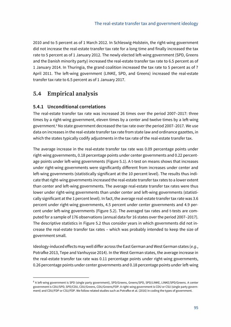
The real-estate transfer tax and government ideology
95
2010 and to 5 percent as of 1 March 2012. In Schleswig-Holstein, the right-wing government
did not increase the real-estate transfer tax rate for a long time and finally increased the tax
rate to 5 percent as of 1 January 2012. The newly elected left-wing government (SPD, Greens
and the Danish minority party) increased the real-estate transfer tax rate to 6.5 percent as of
1 January 2014. In Thuringia, the grand coalition increased the tax rate to 5 percent as of 7
April 2011. The left-wing government (LINKE, SPD, and Greens) increased the real-estate
transfer tax rate to 6.5 percent as of 1 January 2017.
Empirical analysis
5.4.1 Unconditional correlations
The real-estate transfer tax rate was increased 26 times over the period 2007–2017: three
times by a right-wing government, eleven times by a center and twelve times by a left-wing
government.6 No state government decreased the tax rate over the period 2007–2017. We use
data on increases in the real-estate transfer tax rate from state law and ordinance gazettes, in
which the states typically codify adjustments in the tax rate of the real-estate transfer tax.
The average increase in the real-estate transfer tax rate was 0.09 percentage points under
right-wing governments, 0.18 percentage points under center governments and 0.22 percent-
age points under left-wing governments (Figure 5.1). A t-test on means shows that increases
under right-wing governments were significantly different from increases under center and
left-wing governments (statistically significant at the 10 percent level). The results thus indi-
cate that right-wing governments increased the real-estate transfer tax rates to a lower extent
than center and left-wing governments. The average real-estate transfer tax rates were thus
lower under right-wing governments than under center and left-wing governments (statisti-
cally significant at the 1 percent level). In fact, the average real-estate transfer tax rate was 3.6
percent under right-wing governments, 4.5 percent under center governments and 4.9 per-
cent under left-wing governments (Figure 5.2). The averaged tax rates and t-tests are com-
puted for a sample of 176 observations (annual data for 16 states over the period 2007–2017).
The descriptive statistics in Figure 5.2 thus consider years in which governments did not in-
crease the real-estate transfer tax rates – which was probably intended to keep the size of
government small.
Ideology-induced effects may well differ across the East German and West German states (e.g.,
Potrafke 2013, Tepe and Vanhuysse 2014). In the West German states, the average increase in
the real-estate transfer tax rate was 0.11 percentage points under right-wing governments,
0.26 percentage points under center governments and 0.18 percentage points under left-wing
6 A left-wing government is SPD (single party government), SPD/Greens, Greens/SPD, SPD/LINKE, LINKE/SPD/Greens. A center
government is CDU/SPD, SPD/CDU, CDU/Greens, CDU/Greens/FDP. A right-wing government is CDU or CSU (single party govern-
ment) and CDU/FDP or CSU/FDP. We follow related studies such as Potrafke et al. (2016) in coding the types of government.
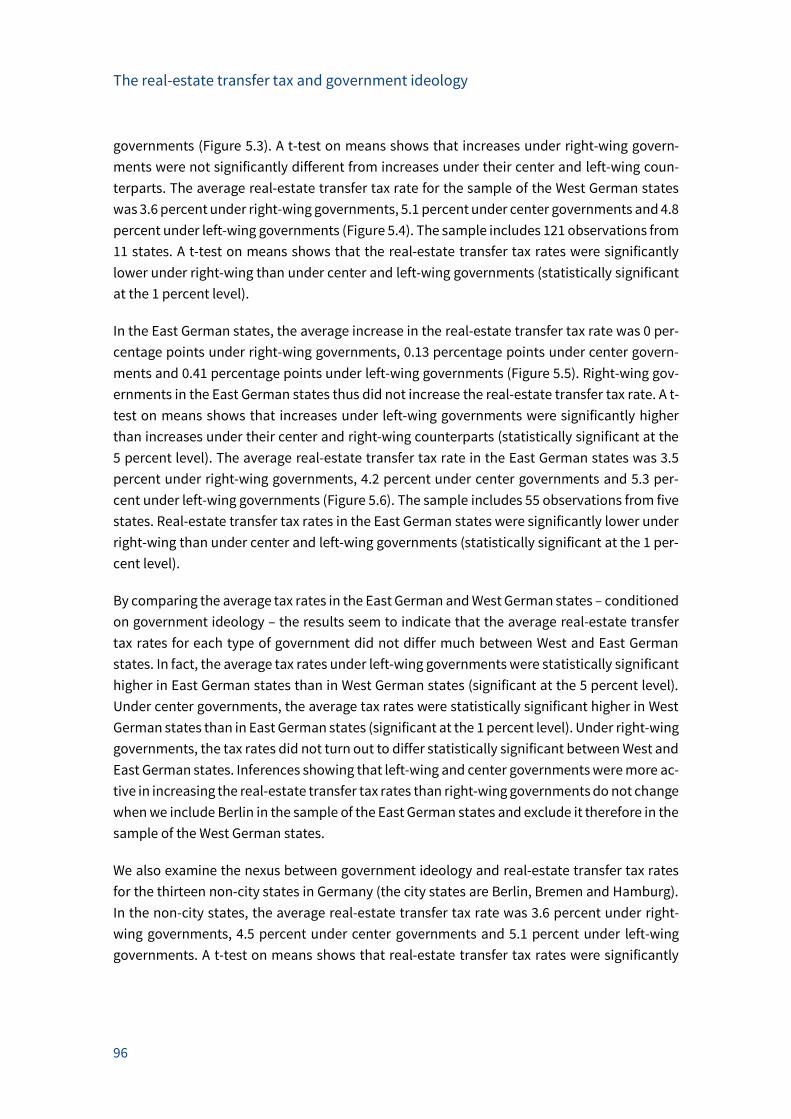
The real-estate transfer tax and government ideology
96
governments (Figure 5.3). A t-test on means shows that increases under right-wing govern-
ments were not significantly different from increases under their center and left-wing coun-
terparts. The average real-estate transfer tax rate for the sample of the West German states
was 3.6 percent under right-wing governments, 5.1 percent under center governments and 4.8
percent under left-wing governments (Figure 5.4). The sample includes 121 observations from
11 states. A t-test on means shows that the real-estate transfer tax rates were significantly
lower under right-wing than under center and left-wing governments (statistically significant
at the 1 percent level).
In the East German states, the average increase in the real-estate transfer tax rate was 0 per-
centage points under right-wing governments, 0.13 percentage points under center govern-
ments and 0.41 percentage points under left-wing governments (Figure 5.5). Right-wing gov-
ernments in the East German states thus did not increase the real-estate transfer tax rate. A t-
test on means shows that increases under left-wing governments were significantly higher
than increases under their center and right-wing counterparts (statistically significant at the
5 percent level). The average real-estate transfer tax rate in the East German states was 3.5
percent under right-wing governments, 4.2 percent under center governments and 5.3 per-
cent under left-wing governments (Figure 5.6). The sample includes 55 observations from five
states. Real-estate transfer tax rates in the East German states were significantly lower under
right-wing than under center and left-wing governments (statistically significant at the 1 per-
cent level).
By comparing the average tax rates in the East German and West German states – conditioned
on government ideology – the results seem to indicate that the average real-estate transfer
tax rates for each type of government did not differ much between West and East German
states. In fact, the average tax rates under left-wing governments were statistically significant
higher in East German states than in West German states (significant at the 5 percent level).
Under center governments, the average tax rates were statistically significant higher in West
German states than in East German states (significant at the 1 percent level). Under right-wing
governments, the tax rates did not turn out to differ statistically significant between West and
East German states. Inferences showing that left-wing and center governments were more ac-
tive in increasing the real-estate transfer tax rates than right-wing governments do not change
when we include Berlin in the sample of the East German states and exclude it therefore in the
sample of the West German states.
We also examine the nexus between government ideology and real-estate transfer tax rates
for the thirteen non-city states in Germany (the city states are Berlin, Bremen and Hamburg).
In the non-city states, the average real-estate transfer tax rate was 3.6 percent under right-
wing governments, 4.5 percent under center governments and 5.1 percent under left-wing
governments. A t-test on means shows that real-estate transfer tax rates were significantly
The real-estate transfer tax and government ideology
97
different under right-wing than under center and left-wing governments (statistically signifi-
cant at the 1 percent level).
5.4.2 Conditional correlations
We investigate the correlation between government ideology and real-estate transfer tax
rates conditional to other variables. The baseline panel-data model has the following form:
Tax ratei,t = β Government ideologyi,t-1
+ γ Voter preferencesi,t + δ Debt per capitai,t-1 + ε Shared taxes per capitai,t-1
+ ηi + τt + ui,t
with i = 1,…,16; t = 1,…,11
where Tax ratei,t measures the tax rate of the real-estate transfer tax in state i and year t. Gov-
ernment ideologyi,t-1 measures ideology-induced policy-making and assumes the value 1 when
a left-wing government was in office, the value 0.5 for a center government, and the value 0
for a right-wing government (e.g., Kauder and Potrafke 2013). We use the government variable
measured in period t-1 because decisions on the tax rates are usually taken in the year before
the adjustment takes place.7 We use the variable Voter preferencesi,t, which measures the
share of right-wing voters (CDU/CSU and FDP) in federal elections. We do so to disentangle
the effect of government ideology and voter preferences on tax policy (see, e.g., Elinder and
Jordahl 2013, Liang 2013, or Freier and Odendahl 2015). We use the vote shares of the last
federal election for each state. It is conceivable that governments use the possibility to in-
crease tax rates for budget consolidation – especially with regard to fulfilling the German debt
brake in 2020.8 An indicator to evaluate the budgetary situation of the states with regard to
the debt brake is the level of debt per capita. We therefore include a variable Debt per capitai,t-
1, which measures the amount of debt per capita of the respective state from the previous
year. The lion’s share of the states’ tax revenues are shared taxes (i.e., income taxes, corporate
taxes and the value added taxes). The state governments have basically no authority to design
the tax policies of the shared taxes and may thus have an incentive to increase the real-estate
transfer tax rate when the share of the shared taxes decreases. We therefore include the
amount of the shared taxes per capita as another explanatory variable (Shared taxes per cap-
itai,t-1). The variables Debt per capitai,t-1 and Shared taxes per capitai,t-1 are measured in period
t-1. We also include fixed time and fixed state effects. We estimate the fixed-effects model with
standard errors robust to heteroskedasticity (Huber/White/sandwich standard errors – see
Huber 1967 and White 1980).
7 In some cases, the decision on and the adjustment of the tax rate took place in the same year. We always consider the govern-
ment which decided on the tax adjustment.
8 A new law on German debt brakes implemented in 2009 states that the state governments are not allowed to run structural
deficits after 2020. The states can choose different consolidation strategies to fulfill the debt brake after 2020. One possibility is
to increase the revenues of the state by increasing the tax rates of the real-estate transfer tax (Potrafke et al. 2016).
The real-estate transfer tax and government ideology
98
Table 5.2 shows descriptive statistics of the individual variables. Table 5.3 shows the correla-
tion coefficients between our variables. Government ideology and the real-estate transfer tax
rates are positively correlated (the coefficient of correlation is 0.499), which is statistically sig-
nificant at the 1 percent level. The real-estate transfer tax rates are also positively correlated
with Debt per capita and Shared taxes per capita, but negatively with the variable measuring
the share of right-wing voters in federal elections.
Table 5.4 shows the regression results excluding fixed time effects. In discussing the results,
we focus on our preferred specification including all control variables in Column (4). The co-
efficient of Government ideology is positive and statistically significant at the 1 percent level.
The tax rate of the real-estate transfer tax is 0.75 percentage points higher under left-wing
than under right-wing and center governments. Focusing on the control variables, the coeffi-
cients for Debt per capita and Shared taxes per capita are significant. The coefficients are, how-
ever, very small. Based on the regression results, Figure 5.7 shows the average tax rates under
right-wing, center and left-wing governments conditional to voter preferences (the vote
shares for the CDU/CSU and the FDP in federal elections), the debt per capita ratio, the shared
taxes per capita ratio in the states and fixed state effects.
In Table 5.5 we include fixed time effects. The coefficient of the government ideology variable
is positive and statistically significant at the 5 percent level indicating that the real-estate
transfer tax rate is 0.52 percentage points higher under left-wing than under right-wing and
center governments. The coefficients of Debt per capita and Shared taxes per capita do not
turn out to be statistically significant. Based on the regression results, Figure 5.8 shows the
average tax rates under right-wing, center and left-wing governments conditional to voter
preferences, the debt per capita ratio, the shared taxes per capita ratio and fixed time and
state effects.
5.4.3 Robustness tests
We submitted our results to rigorous robustness tests. We investigate the correlation between
government ideology and the first difference in the real-estate transfer tax rates conditional
to other variables. The conditional correlation between government ideology in period t-1 and
the first difference in the real-estate transfer tax rates is positive and statistically significant
at the 10 percent level, when we condition on the vote shares for the CDU/CSU and the FDP in
federal elections (Voter preferences), the debt per capita ratio, the shared taxes per capita ra-
tio and state-fixed effects. Inferences do not change when we include fixed time effects.
We also condition the correlation between government ideology and the real-estate transfer
tax rate on demographic variables by taking into account the share of young citizens up to 20
years and the share of old citizens above 60 years. The real-estate transfer tax might affect age
classes in different ways depending on whether they already own property. Thus, state gov-
ernments may well consider the age distribution within a state when deciding on tax rates.
The real-estate transfer tax and government ideology
99
Firstly, by excluding fixed time effects but including fixed state effects, the correlation be-
tween Government ideology and the real-estate transfer tax rate is positive and statistically
significant at the 1 percent level. When fixed time effects are also included, the correlation
between Government ideology and the real-estate transfer tax rate remains positive and sta-
tistically significant at the 5 percent level. Focusing on the demographic variables, the coeffi-
cient for the share of old citizens is positive and statistically significant only when excluding
fixed time effects. The coefficient for the share of young citizens is negative and statistically
significant at the 5 percent level when including fixed time effects. We also include the share
of left-wing voters (SPD, Greens, and Left Party) instead of the share of right-wing voters in
federal elections. Inferences do not change regarding Government ideology. The results show
that government ideology is significantly correlated with the real-estate transfer tax rates also
when conditioning on other variables.
We also examine the increases in the real-estate transfer tax rates by the type of government
on the basis of legislative periods. There were 35 different full legislative periods between
2007 and 2017. The average increase in the real-estate transfer tax rate is 0.31 percentage
points lower under right-wing than under left-wing governments. The difference in the in-
creases of the tax rates under left-wing and right-wing governments is statistically significant
at the 1 percent level. We also examine the increases in the real-estate transfer tax rates on
the basis of cabinet periods (Schmitt 2015) to take into account the duration of the respective
governments in each state. There were 62 different cabinets in the time period between 2007
and 2017. The average increase under left-wing governments was significantly higher than
under right-wing and center governments (statistically significant at the 10 percent level). In
fact, the average increase based on cabinet periods was 0.08 percentage points under right-
wing, 0.14 percentage points under center and 0.24 percentage points under left-wing gov-
ernments.
Governments might postpone tax rate increases until after elections because of electoral mo-
tives.9 We examine electoral cycles in the timing of the decision on tax rate increases. The real-
estate transfer tax rate was increased 26 times over the period 2007–2017. Out of the 26 deci-
sions, 5 decisions on tax rate increases took place in an election year; another 3 decisions took
place in the pre-election year, while 11 decisions were taken after an election year.10 To exam-
ine the effect of electoral motives on real-estate transfer tax rate increases in more detail, we
include dummy variables for the individual types of years in the regressions (pre-election year,
election year, post-election year). The coefficient of the pre-election year dummy variable is
9 The political business cycle theories describe that election-motivated politicians pursue expansionary policies before elections.
For example, politicians may increase public spending or decrease taxes (Nordhaus 1975, Rogoff and Sibert 1988, Rogoff 1990;
see De Haan and Klomp 2013 for a survey on studies dealing with political business cycles).
10 Decisions on increases in the real-estate transfer tax rate in an election year always took place after the election. In case of
early elections, we consider the decision on the tax rate increase only as belonging to the pre-election year when early elections
were known at that point of time.
The real-estate transfer tax and government ideology
100
negative but lacks statistical significance – including/excluding fixed time effects notwith-
standing – when we use the increases in the real-estate transfer tax rates as the dependent
variable. This holds also true for the election year dummy variable. The coefficient of the post-
election year variable is positive and statistically significant at the 10 percent level indicating
that governments postpone tax rate increases until after elections. Inferences with regard to
the election dummy variables do not change when we include all election dummy variables
at the same time. By including the election variables, the government ideology variable re-
mains positive but does not turn out to be statistically significant at conventional levels.
We also examined whether our results are driven by individual years or individual states. When
we exclude individual years or states, one at a time (jackknife test), the results still show a
positive and significant correlation between the government ideology variable and the real-
estate transfer tax rates.
Conclusion
In 2006, the German fiscal constitution was reformed. The reform allowed the German state
governments to set the real-estate transfer tax rates (the tax rate was 3.5 percent at the end
of 2006). The reform lends itself to an examination because German state governments have
had hardly any tools for determining tax rates. Allowing the German state governments to set
the rates of the real-estate transfer tax is an excellent case in point to investigate whether
government ideology predicts economic policy-making. The real-estate transfer tax is likely
to influence high-income citizens (often voters of right-wing parties) to a larger extent than
low-income citizens (often voters of left-wing parties). We focus on case study evidence and a
descriptive correlational analysis in the 16 German states because we cannot derive causal
effects in the small sample. The results show that right-wing governments were less active in
increasing the real-estate transfer tax rates than left-wing and center governments. Over the
period 2007–2017, the real-estate transfer tax rate was increased 26 times: three times under
right-wing governments, eleven times under center governments and twelve times under left-
wing governments. The average tax rate was 3.6 percent under right-wing governments, 4.5
percent under center governments and 4.9 percent under left-wing governments. Bavaria and
Saxony, two German states with quite conservative electorates (and governments), did not
increase the real-estate transfer tax rate over the period 2007–2017. In Baden-Wuerttemberg
and North Rhine-Westphalia the newly elected left-wing governments increased the real-es-
tate transfer tax rates when following right-wing governments. We also examine the correla-
tion between government ideology and real-estate transfer tax rates conditional to other var-
iables. The results show that government ideology is correlated with the real-estate transfer
tax rates when taking into account other variables such as fixed state and time effects, public
debt per capita, shared taxes per capita, voter preferences and demographic variables.
The real-estate transfer tax and government ideology
101
Government ideology retired to the background at the federal level. There has hardly been
any difference in the policies pursued by CDU- and SPD-led federal governments since the
1990s (e.g., Zohlnhöfer 2003, Potrafke 2012, Kauder and Potrafke 2016). Many voters were dis-
enchanted by the catch-all policies of the CDU and SPD; in the early 2000s, the populist left-
wing party (DIE LINKE) entered the political arena and gained some electoral support. In 2015
and 2016, the populist right-wing Alternative for Germany was successful in many state elec-
tions. With polarized tax policies of CDU/CSU and SPD-led state governments, voters may well
find the established parties attractive, rather than supporting parties at the fringe of the po-
litical spectrum.
We have conjectured that voters of left-wing parties are more inclined to increase the real-
estate transfer tax rates than voters of right-wing parties. Future research may well compile
survey evidence describing the nexus between political ideologies and voters’ preferences re-
garding the real-estate transfer tax.
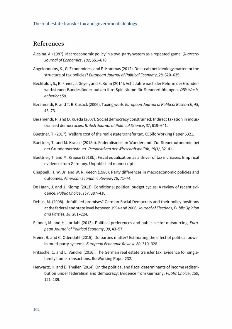
The real-estate transfer tax and government ideology
102
References
Alesina, A. (1987). Macroeconomic policy in a two-party system as a repeated game. Quarterly
Journal of Economics, 102, 651–678.
Angelopoulos, K., G. Economides, and P. Kammas (2012). Does cabinet ideology matter for the
structure of tax policies? European Journal of Political Economy, 28, 620–635.
Bechtoldt, S., R. Freier, J. Geyer, and F. Kühn (2014). Acht Jahre nach der Reform der Grunder-
werbsteuer: Bundesländer nutzen ihre Spielräume für Steuererhöhungen. DIW Woch-
enbericht 50.
Beramendi, P. and T. R. Cusack (2006). Taxing work. European Journal of Political Research, 45,
43–73.
Beramendi, P. and D. Rueda (2007). Social democracy constrained: Indirect taxation in indus-
trialized democracies. British Journal of Political Science, 37, 619–641.
Buettner, T. (2017). Welfare cost of the real estate transfer tax. CESifo Working Paper 6321.
Buettner, T. and M. Krause (2018a). Föderalismus im Wunderland: Zur Steuerautonomie bei
der Grunderwerbsteuer. Perspektiven der Wirtschaftspolitik, 19(1), 32–41.
Buettner, T. and M. Krause (2018b). Fiscal equalization as a driver of tax increases: Empirical
evidence from Germany. Unpublished manuscript.
Chappell, H. W. Jr. and W. R. Keech (1986). Party differences in macroeconomic policies and
outcomes. American Economic Review, 76, 71–74.
De Haan, J. and J. Klomp (2013). Conditional political budget cycles: A review of recent evi-
dence. Public Choice, 157, 387–410.
Debus, M. (2008). Unfulfilled promises? German Social Democrats and their policy positions
at the federal and state level between 1994 and 2006. Journal of Elections, Public Opinion
and Parties, 18, 201–224.
Elinder, M. and H. Jordahl (2013). Political preferences and public sector outsourcing. Euro-
pean Journal of Political Economy, 30, 43–57.
Freier, R. and C. Odendahl (2015). Do parties matter? Estimating the effect of political power
in multi-party systems. European Economic Review, 80, 310–328.
Fritzsche, C. and L. Vandrei (2016). The German real estate transfer tax: Evidence for single-
family home transactions. Ifo Working Paper 232.
Herwartz, H. and B. Theilen (2014). On the political and fiscal determinants of income redistri-
bution under federalism and democracy: Evidence from Germany. Public Choice, 159,
121–139.
The real-estate transfer tax and government ideology
103
Hibbs, D. A. Jr. (1977). Political parties and macroeconomic policy. American Political Science
Review, 71, 1467–1487.
Hildebrandt, A. (2016). Die Finanzpolitik der Länder nach den Föderalismusreformen: Be-
grenzte Spielräume, fortdauernde Unterschiede. In: A. Hildebrandt and F. Wolf (Eds.),
Die Politik der Bundesländer. Zwischen Föderalismusreform und Schuldenbremse. Wies-
baden: Springer VS, pp. 115–137.
Huber, P. J. (1967). The behavior of maximum likelihood estimates under nonstandard condi-
tions. In: Proceedings of the Fifth Berkeley Symposium on Mathematical Statistics and
Probability, pp. 221–233.
Jäger, K. (2017). Economic freedom in the early 21st century: Government ideology still mat-
ters. Kyklos, 70, 256–277.
Jochimsen, B. and R. Nuscheler (2011). The political economy of the German Lander deficits:
Weak governments meet strong finance ministers. Applied Economics, 43, 2399–2415.
Jochimsen, B. and S. Thomasius (2014). The perfect finance minister: Whom to appoint as fi-
nance minister to balance the budget? European Journal of Political Economy, 34, 390–
408.
Kauder, B. and N. Potrafke (2013). Government ideology and tuition fee policy: Evidence from
the German states. CESifo Economic Studies, 59, 628–649.
Kauder, B. and N. Potrafke (2016). The growth in military expenditure in Germany 1950–2011:
Did parties matter? Defence and Peace Economics, 27, 503–519.
Koester, G. B. (2009). The Political Economy of Tax Reforms: An Empirical Analysis of New Ger-
man Data. Baden-Baden: Nomos Verlagsgesellschaft.
Liang, C.-Y. (2013). Is there an incumbency advantage or cost of ruling in proportional election
systems? Public Choice, 154, 259–284.
Nordhaus, W. D. (1975). The political business cycle. Review of Economic Studies, 42, 169–190.
Oberndorfer, U. and V. Steiner (2007). Generationen- oder Parteienkonflikt? Eine empirische
Analyse der deutschen Hochschulausgaben. Perspektiven der Wirtschaftspolitik, 8, 165–
183.
Osterloh, S. and M. Debus (2012). Partisan politics in corporate taxation. European Journal of
Political Economy, 28, 192–207.
Petkova, K. and A. Weichenrieder (2017). Price and quantity effects of the German real estate
transfer tax. CESifo Working Paper 6538.
Potrafke, N. (2011). Public expenditures on education and cultural affairs in the West German
states: Does government ideology influence the budget composition? German Eco-
nomic Review, 12, 124–145.
The real-estate transfer tax and government ideology
104
Potrafke, N. (2012). Is German domestic social policy politically controversial? Public Choice,
153, 393–418.
Potrafke, N. (2013). Economic freedom and government ideology across the German states.
Regional Studies, 47, 433–449.
Potrafke, N. (2017). Partisan politics: The empirical evidence from OECD panel studies. Jour-
nal of Comparative Economics, 45, 712–750.
Potrafke, N. (2018). Government ideology and economic policy-making in the United States –
A survey. Public Choice, 174, 145–207.
Potrafke, N., M. Riem, and C. Schinke (2016). Debt brakes in the Germans states: Governments’
rhetoric and actions. German Economic Review, 17, 253–275.
Quinn, D. P. and R. Y. Shapiro (1991). Economic growth strategies: The effects of ideological
partisanship on interest rates and business taxation in the United States. American
Journal of Political Science, 35, 656–685.
Roesel, F. (2017). The political economy of fiscal supervision and budget deficits – Evidence
from Germany. Fiscal Studies, 38, 641–666.
Rogoff, K. (1990). Equilibrium political budget cycles. American Economic Review, 80, 21–36.
Rogoff, K. and A. Sibert (1988). Elections and macroeconomic policy cycles. Review of Eco-
nomic Studies, 55, 1–16.
Schmitt, C. (2015). Panel data analysis and partisan variables: How periodization does influ-
ence partisan effects. Journal of European Public Policy, 23, 1442–1459.
Schmitt, C. and R. Zohlnhöfer (2018). Partisan differences and the interventionist state in ad-
vanced democracies. Socio-Economic Review, forthcoming.
Tepe, M. and P. Vanhuysse (2013). Cops for hire? The political economy of police employment
in the German states. Journal of Public Policy, 33, 165–199.
Tepe, M. and P. Vanhuysse (2014). A vote at the opera? The political economy of public thea-
ters and orchestras in the German states. European Journal of Political Economy, 36,
254–273.
White, H. (1980). A heteroskedasticity-consistent covariance matrix estimator and a direct test
for heteroskedasticity. Econometrica, 48, 817–838.
Zohlnhöfer, R. (2003). Partisan politics, political competition, and veto players: German eco-
nomic policy in the Kohl era. Journal of Public Policy, 23, 123–156.
Zohlnhöfer, R., F. Engler, and K. Dümig (2018). The retreat of the interventionist state in ad-
vanced democracies. British Journal of Political Science, 48, 535–562.
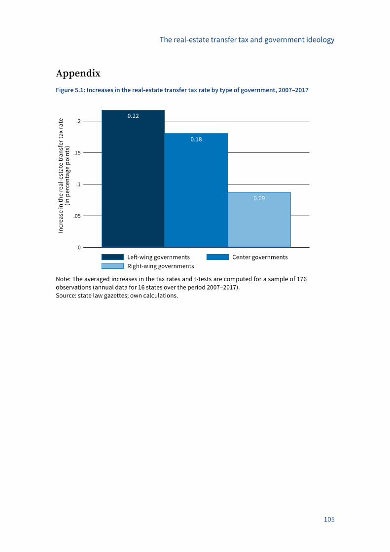
The real-estate transfer tax and government ideology
105
Appendix
Figure 5.1: Increases in the real-estate transfer tax rate by type of government, 2007–2017
Note: The averaged increases in the tax rates and t-tests are computed for a sample of 176
observations (annual data for 16 states over the period 2007–2017).
Source: state law gazettes; own calculations.
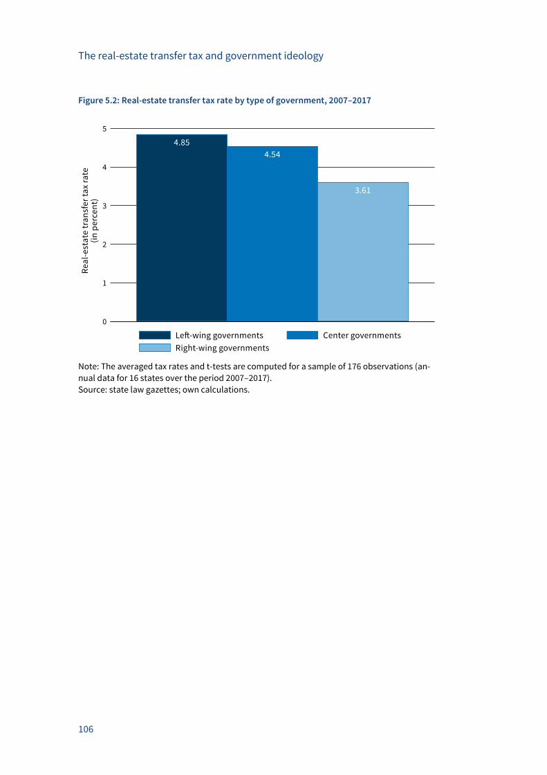
The real-estate transfer tax and government ideology
106
Figure 5.2: Real-estate transfer tax rate by type of government, 2007–2017
Note: The averaged tax rates and t-tests are computed for a sample of 176 observations (an-
nual data for 16 states over the period 2007–2017).
Source: state law gazettes; own calculations.
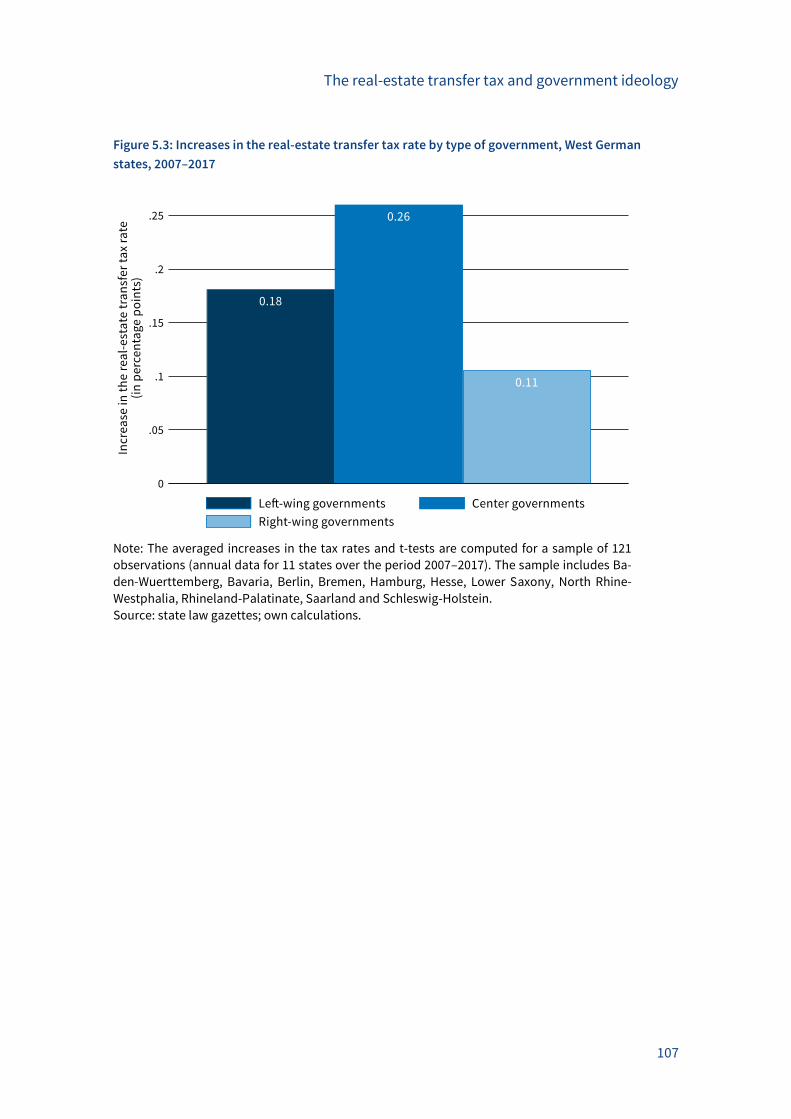
The real-estate transfer tax and government ideology
107
Figure 5.3: Increases in the real-estate transfer tax rate by type of government, West German
states, 2007–2017
Note: The averaged increases in the tax rates and t-tests are computed for a sample of 121
observations (annual data for 11 states over the period 2007–2017). The sample includes Ba-
den-Wuerttemberg, Bavaria, Berlin, Bremen, Hamburg, Hesse, Lower Saxony, North Rhine-
Westphalia, Rhineland-Palatinate, Saarland and Schleswig-Holstein.
Source: state law gazettes; own calculations.
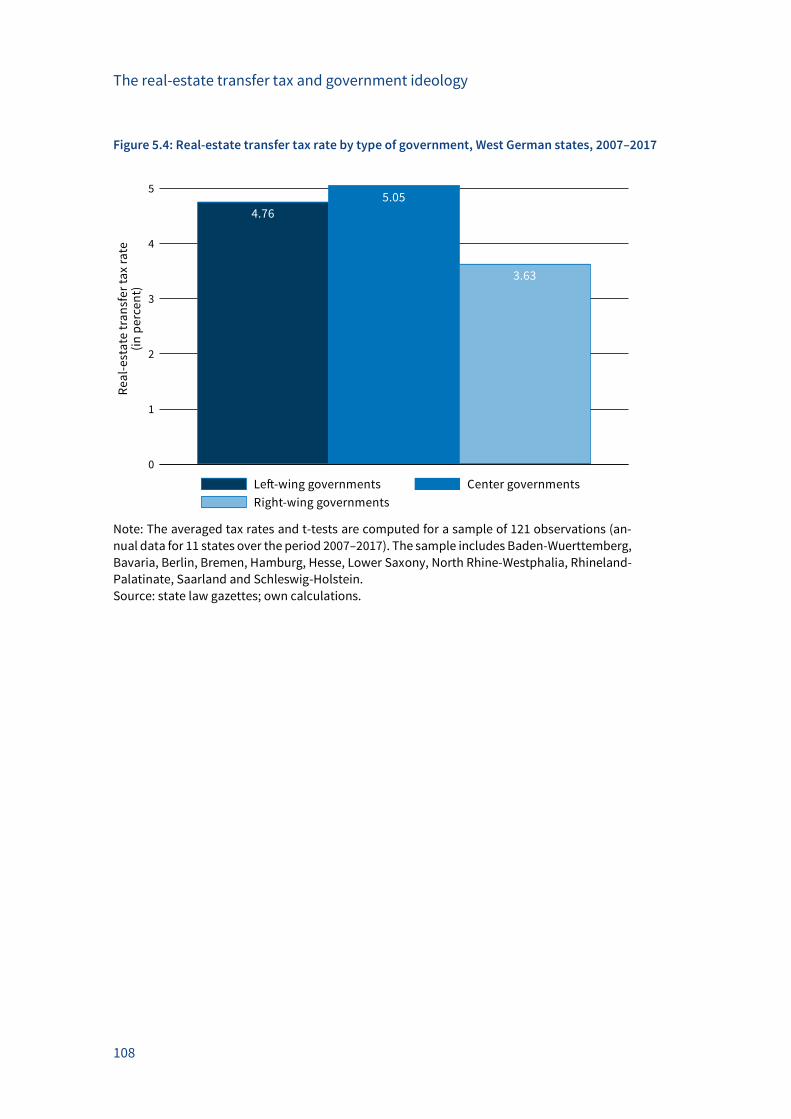
The real-estate transfer tax and government ideology
108
Figure 5.4: Real-estate transfer tax rate by type of government, West German states, 2007–2017
Note: The averaged tax rates and t-tests are computed for a sample of 121 observations (an-
nual data for 11 states over the period 2007–2017). The sample includes Baden-Wuerttemberg,
Bavaria, Berlin, Bremen, Hamburg, Hesse, Lower Saxony, North Rhine-Westphalia, Rhineland-
Palatinate, Saarland and Schleswig-Holstein.
Source: state law gazettes; own calculations.
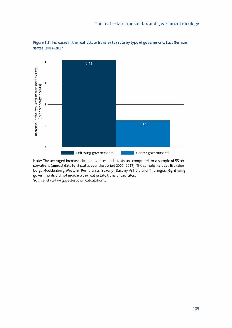
The real-estate transfer tax and government ideology
109
Figure 5.5: Increases in the real-estate transfer tax rate by type of government, East German
states, 2007–2017
Note: The averaged increases in the tax rates and t-tests are computed for a sample of 55 ob-
servations (annual data for 5 states over the period 2007–2017). The sample includes Branden-
burg, Mecklenburg-Western Pomerania, Saxony, Saxony-Anhalt and Thuringia. Right-wing
governments did not increase the real-estate transfer tax rates.
Source: state law gazettes; own calculations.
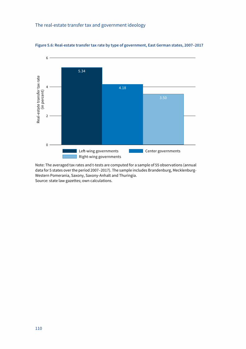
The real-estate transfer tax and government ideology
110
Figure 5.6: Real-estate transfer tax rate by type of government, East German states, 2007–2017
Note: The averaged tax rates and t-tests are computed for a sample of 55 observations (annual
data for 5 states over the period 2007–2017). The sample includes Brandenburg, Mecklenburg-
Western Pomerania, Saxony, Saxony-Anhalt and Thuringia.
Source: state law gazettes; own calculations.
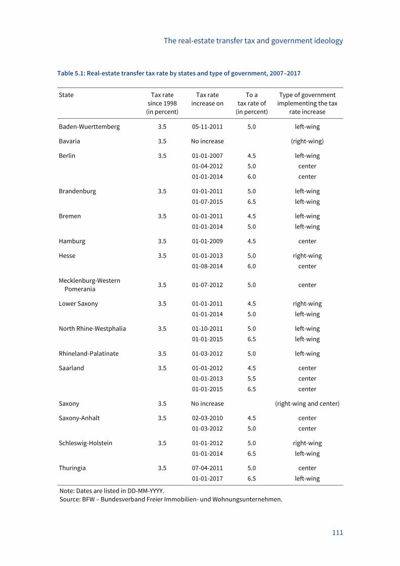
The real-estate transfer tax and government ideology
111
Table 5.1: Real-estate transfer tax rate by states and type of government, 2007–2017
State Tax rate
since 1998
(in percent)
Tax rate
increase on
To a
tax rate of
(in percent)
Type of government
implementing the tax
rate increase
Baden-Wuerttemberg 3.5 05-11-2011 5.0 left-wing
Bavaria 3.5 No increase (right-wing)
Berlin 3.5 01-01-2007 4.5 left-wing 01-04-2012 5.0 center
01-01-2014 6.0 center
Brandenburg 3.5 01-01-2011 5.0 left-wing
01-07-2015 6.5 left-wing
Bremen 3.5 01-01-2011 4.5 left-wing
01-01-2014 5.0 left-wing
Hamburg 3.5 01-01-2009 4.5 center
Hesse 3.5 01-01-2013 5.0 right-wing
01-08-2014 6.0 center
Mecklenburg-Western
Pomerania 3.5 01-07-2012 5.0 center
Lower Saxony 3.5 01-01-2011 4.5 right-wing
01-01-2014 5.0 left-wing
North Rhine-Westphalia 3.5 01-10-2011 5.0 left-wing
01-01-2015 6.5 left-wing
Rhineland-Palatinate 3.5 01-03-2012 5.0 left-wing
Saarland 3.5 01-01-2012 4.5 center 01-01-2013 5.5 center
01-01-2015 6.5 center
Saxony 3.5 No increase (right-wing and center)
Saxony-Anhalt 3.5 02-03-2010 4.5 center
01-03-2012 5.0 center
Schleswig-Holstein 3.5 01-01-2012 5.0 right-wing
01-01-2014 6.5 left-wing
Thuringia 3.5 07-04-2011 5.0 center
01-01-2017 6.5 left-wing
Note: Dates are listed in DD-MM-YYYY.
Source: BFW – Bundesverband Freier Immobilien- und Wohnungsunternehmen.
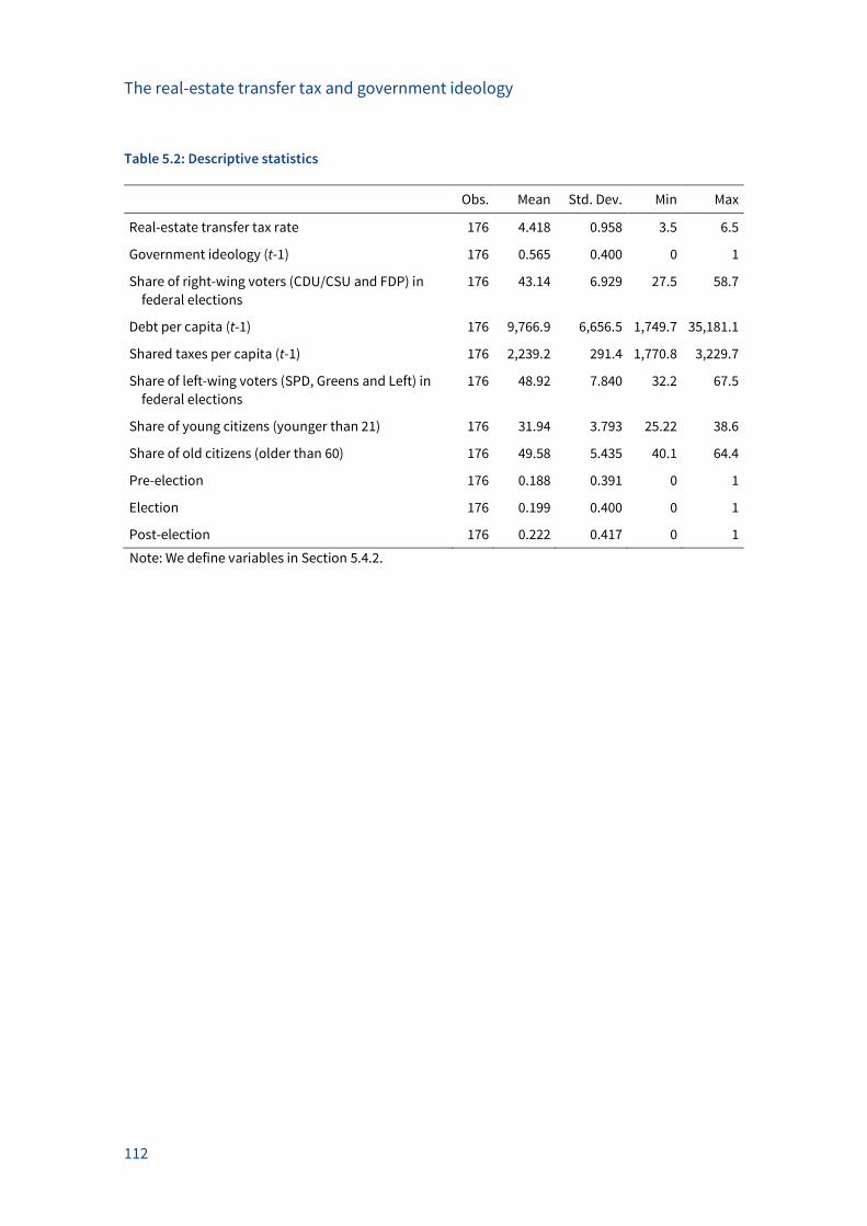
The real-estate transfer tax and government ideology
112
Table 5.2: Descriptive statistics
Obs. Mean Std. Dev. Min Max
Real-estate transfer tax rate 176 4.418 0.958 3.5 6.5
Government ideology (t-1) 176 0.565 0.400 0 1
Share of right-wing voters (CDU/CSU and FDP) in
federal elections
176 43.14 6.929 27.5 58.7
Debt per capita (t-1) 176 9,766.9 6,656.5 1,749.7 35,181.1
Shared taxes per capita (t-1) 176 2,239.2 291.4 1,770.8 3,229.7
Share of left-wing voters (SPD, Greens and Left) in
federal elections
176 48.92 7.840 32.2 67.5
Share of young citizens (younger than 21) 176 31.94 3.793 25.22 38.6
Share of old citizens (older than 60) 176 49.58 5.435 40.1 64.4
Pre-election 176 0.188 0.391 0 1
Election 176 0.199 0.400 0 1
Post-election 176 0.222 0.417 0 1
Note: We define variables in Section 5.4.2.
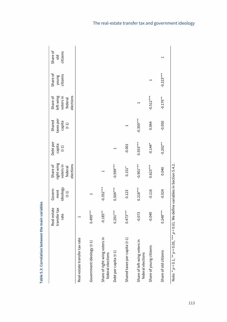
The real-estate transfer tax and government ideology
113
Ta
ble
5.3
: Co
rre
lati
on
be
twe
en
th
e m
ain
va
ria
ble
s
R
eal-
esta
te
tra
nsf
er t
ax
rate
Go
vern
-
men
t
ideo
log
y
(t-1
)
Sh
are
of
rig
ht-
win
g
vote
rs in
fed
era
l
elec
tio
ns
Deb
t p
er
cap
ita
(t-1
)
Sh
are
d
taxe
s p
er
cap
ita
(t-1
)
Sh
are
of
left
-win
g
vote
rs in
fed
era
l
elec
tio
ns
Sh
are
of
you
ng
citi
zen
s
Sh
are
of
old
citi
zen
s
Rea
l-es
tate
tra
nsf
er t
ax
rate
1
Go
vern
men
t id
eo
log
y (t
-1)
0.49
9***
1
Sh
are
of r
igh
t-w
ing
vo
ters
in
fed
era
l ele
ctio
ns
-0.1
85**
-0
.352
***
1
Deb
t p
er c
ap
ita
(t-
1)
0.29
1***
0.
504*
**
-0.5
99**
* 1
Sh
are
d t
axe
s p
er c
ap
ita
(t-
1)
0.47
3***
0.
123
0.
151*
-0
.001
1
Sh
are
of l
eft-
win
g v
ote
rs in
fed
era
l ele
ctio
ns
-0.0
73
0.21
8***
-0
.901
***
0.55
3***
-0
.359
***
1
Sh
are
of y
ou
ng
cit
izen
s
-0.0
49
-0.1
16
0.62
3***
-0
.144
* 0.
064
-0
.512
***
1
Sh
are
of o
ld c
itiz
en
s
0.24
8***
-0
.024
0.
040
-0
.202
**
-0.0
50
-0.1
76**
-0
.223
***
1
No
te: *
p <
0.1
, **
p <
0.0
5, *
** p
< 0
.01.
We
de
fin
e va
ria
ble
s in
Sec
tio
n 5
.4.2
.
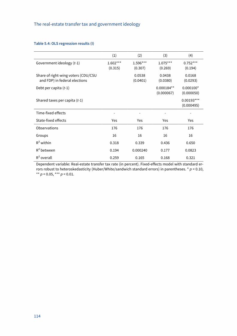
The real-estate transfer tax and government ideology
114
Table 5.4: OLS regression results (I)
(1) (2) (3) (4)
Government ideology (t-1) 1.602*** 1.596*** 1.075*** 0.752***
(0.315) (0.307) (0.269) (0.194)
Share of right-wing voters (CDU/CSU
and FDP) in federal elections
0.0538 0.0438 0.0168
(0.0401) (0.0380) (0.0293)
Debt per capita (t-1) 0.000184** 0.000100*
(0.000067) (0.000050)
Shared taxes per capita (t-1)
0.00193***
(0.000495)
Time-fixed effects - - - -
State-fixed effects Yes Yes Yes Yes
Observations 176 176 176 176
Groups 16 16 16 16
R² within 0.318 0.339 0.436 0.650
R² between 0.194 0.000240 0.177 0.0823
R² overall 0.259 0.165 0.168 0.321
Dependent variable: Real-estate transfer tax rate (in percent). Fixed-effects model with standard er-
rors robust to heteroskedasticity (Huber/White/sandwich standard errors) in parentheses. * p < 0.10,
** p < 0.05, *** p < 0.01.
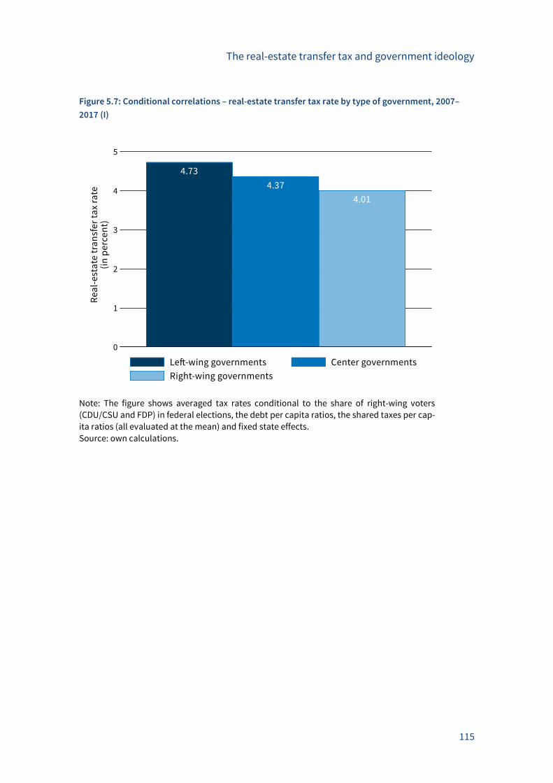
The real-estate transfer tax and government ideology
115
Figure 5.7: Conditional correlations – real-estate transfer tax rate by type of government, 2007–
2017 (I)
Note: The figure shows averaged tax rates conditional to the share of right-wing voters
(CDU/CSU and FDP) in federal elections, the debt per capita ratios, the shared taxes per cap-
ita ratios (all evaluated at the mean) and fixed state effects.
Source: own calculations.
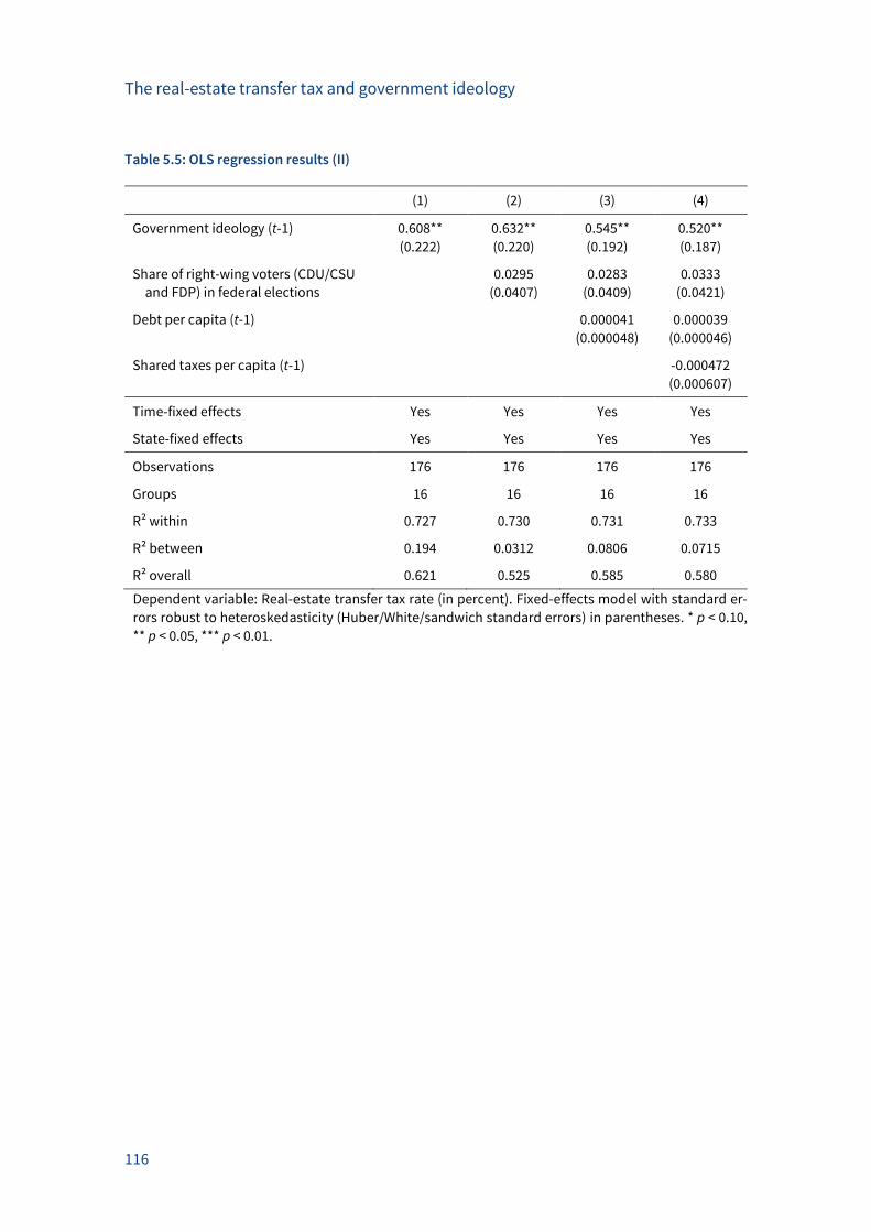
The real-estate transfer tax and government ideology
116
Table 5.5: OLS regression results (II)
(1) (2) (3) (4)
Government ideology (t-1) 0.608** 0.632** 0.545** 0.520**
(0.222) (0.220) (0.192) (0.187)
Share of right-wing voters (CDU/CSU
and FDP) in federal elections
0.0295 0.0283 0.0333
(0.0407) (0.0409) (0.0421)
Debt per capita (t-1) 0.000041 0.000039
(0.000048) (0.000046)
Shared taxes per capita (t-1)
-0.000472
(0.000607)
Time-fixed effects Yes Yes Yes Yes
State-fixed effects Yes Yes Yes Yes
Observations 176 176 176 176
Groups 16 16 16 16
R² within 0.727 0.730 0.731 0.733
R² between 0.194 0.0312 0.0806 0.0715
R² overall 0.621 0.525 0.585 0.580
Dependent variable: Real-estate transfer tax rate (in percent). Fixed-effects model with standard er-
rors robust to heteroskedasticity (Huber/White/sandwich standard errors) in parentheses. * p < 0.10,
** p < 0.05, *** p < 0.01.
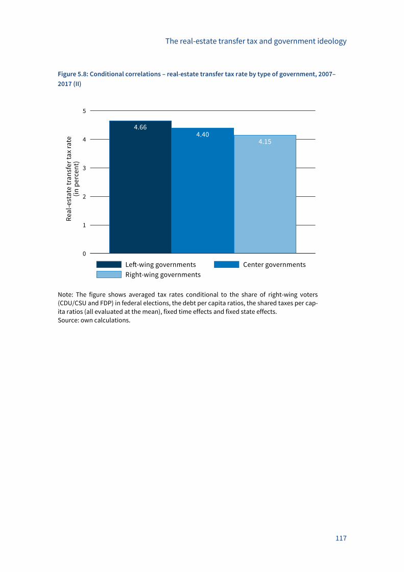
The real-estate transfer tax and government ideology
117
Figure 5.8: Conditional correlations – real-estate transfer tax rate by type of government, 2007–
2017 (II)
Note: The figure shows averaged tax rates conditional to the share of right-wing voters
(CDU/CSU and FDP) in federal elections, the debt per capita ratios, the shared taxes per cap-
ita ratios (all evaluated at the mean), fixed time effects and fixed state effects.
Source: own calculations.

The real-estate transfer tax and government ideology
118
Federalism in Wonderland
119
6 Federalism in Wonderland: Tax autonomy in
German real-estate transfer taxation
Federalism in Wonderland
Abstract*
Using the devolution of tax setting powers to German states since 2006, this chapter examines
the consideration of real-estate transfer tax revenues within the German fiscal equalization
system. We simulate the development of fiscal redistribution within the equalization scheme
for each state from 2006 to 2016. The results show that there is a strong fiscal incentive for
many states to increase their tax rates because they not only receive higher tax revenues, but
also higher transfers. States that do not increase their tax rates experience a paradoxical sit-
uation whereby each additional euro of real-estate transfer tax revenue causes a decrease in
state revenues from transfers that exceeds the increase in tax revenue.
* This chapter is based on joint work with Thiess Büttner. It is based on our paper “Föderalismus im Wunderland: Zur Steuerau-
tonomie bei der Grunderwerbsteuer”, Perspektiven der Wirtschaftspolitik, 19(1), 32–41, 2018. We would like to thank Niklas Po-
trafke for helpful suggestions and comments and Lisa Giani Contini for proof-reading. Kristin Fischer, Tobias Görbert and Felix
Michalik provided excellent research assistance.
Federalism in Wonderland
120
Introduction
A recent federal reform of the German fiscal constitution in 2006 realigned legislative powers
between the federal and the state governments. The reform allowed German states to set the
tax rate of the real-estate transfer tax. The reform aimed to strengthen state governments’
autonomy in taxation, because prior to the reform states could not adjust tax revenues to their
needs. Only municipalities were able to set the tax rates of property and business taxes. The
choice of the real-estate transfer tax was reasonable as it is a state tax whose revenue is ex-
clusively for the states. The states actively used their right to set the tax rates. Since 2006,
most states have raised their tax rates. The real-estate transfer tax rate was increased 25 times
in total prior to 2017. No state has lowered its tax rate.
This development may be an indicator for the states being under substantial revenue stress
and thus adjusting their tax policies accordingly. Krause and Potrafke (2017) also provide ev-
idence for political economic determinants of the real-estate transfer tax policy in recent
years (see also Chapter 5). Taking into account the federal fiscal equalization system, an ad-
ditional explanation becomes evident: the tax autonomy of the states is limited to the extent
that the fiscal equalization scheme still accounts for revenues from real-estate transfer taxes.
This combination provides a conflict between tax autonomy and redistributive fiscal equali-
zation. On the one hand, states have the opportunity to adjust their revenues. On the other
hand, fiscal equalization reduces disparities in fiscal capacity among states. This tension has
implications for the states’ tax policy. The states need to consider how revenues from the real-
estate transfer tax change with an increase in the tax rate. But the states also need to consider
changes in transfers from fiscal equalization. States that make contributions within the equal-
ization scheme have to account for changes in paid transfers, while states that receive trans-
fers must investigate how received transfers change.
The combination of tax autonomy and fiscal equalization may provide incentives for an ex-
cessive taxation (e.g., Buettner and Schwager 2003). This also holds for the real-estate transfer
tax in Germany. The legislator has tried to solve the conflict between tax autonomy and equal-
ization by not using the revenue from the real-estate transfer tax directly within the equaliza-
tion scheme, but by using standardized tax revenues instead. The calculation of states’ reve-
nues from taxes and other contributions (Förderabgaben) within the equalization scheme
thus only considers revenues of the real-estate transfer tax that would arise if an average real-
estate transfer tax rate is applied to the total taxable land and real-estate transactions. In-
creasing or decreasing the own tax rate thus does not give rise to an immediate rise or fall in
the fiscal capacity of a state, which determines transfers within the fiscal equalization
scheme. The use of a representative tax rate does not, however, solve the conflict. Accounting
for real-estate transfer tax revenues within the fiscal equalization scheme still provides strong
incentives to increase the real-estate transfer tax rate. For states that receive transfers, an
increase in the tax rate is related to both an increase in tax revenue and in transfers from the
Federalism in Wonderland
121
fiscal equalization system. For states that make contributions, the contributions within fiscal
equalization decline. A state that does not increase its tax rate to the same extent as the other
states might face a decline in revenues. A paradoxical situation may even arise whereby
states’ revenues decline with every additional euro from real-estate transfer tax revenues be-
cause the transfers decrease so strongly.
We exploit the development of the real-estate transfer tax rate since 2006 to examine the re-
distribution of revenues within the fiscal equalization system by focusing on the real-estate
transfer tax revenues. Employing a comprehensive simulation model, we examine how the
incentives to set the tax rates of the real-estate transfer tax have developed within the fiscal
equalization system since 2006. The results show that the incentives to raise the tax rate have
increased over time, especially for states, which have left the real-estate transfer tax rate un-
changed. Since 2012 the state of Saxony, for example, has been in a situation where every
additional euro of real-estate transfer tax revenue reduces overall financial resources. Accord-
ing to the newest calculations, Saxony loses about 1.38 euro with every additional euro from
the real-estate transfer tax through a decline in transfers within fiscal equalization. It is con-
ceivable that more states will get into such a paradoxical situation if the actual development
in the real-estate transfer tax rates continues. Recent calculations for Bremen and Mecklen-
burg-Western Pomerania – based on the preliminary statistics for the year 2016 – seem to con-
firm this hypothesis.
The economic literature has examined incentives of fiscal redistribution on local tax policies
from a theoretical point of view (see, e.g., Smart 1998, Köthenbürger 2002). Empirical studies
investigate how grants provided to German municipalities influence tax policy of the munici-
palities (e.g., Buettner 2006). How incentives in the fiscal equalization system influence the
setting of the real-estate transfer tax rate has hardly been discussed. The Advisory Board to
the Federal Ministry of Finance highlighted this problem in a report from 2015 (Wissenschaft-
licher Beirat 2015, p. 25). Other studies illustrate the incentives of fiscal equalization by simu-
lating different scenarios and show that the real-estate transfer tax is distorting (Boysen-
Hogrefe 2017; see also Fritzsche and Vandrei 2016, Petkova and Weichenrieder 2017, Buettner
2017b). We focus on determining and examining the degree of fiscal redistribution within fis-
cal equalization, which causes the incentive effect to raise the tax rates.
The following section describes the conflict between tax autonomy and fiscal equalization
and the resulting incentive effect. Section 6.3 develops a measure that calculates the specific
fiscal incentive faced by each state. Section 6.4 briefly outlines the simulation approach. Sec-
tion 6.5 presents the results and quantifies the development of fiscal redistribution over time.
Finally, we briefly discuss how the incentive for excessive taxation in the case of the real-estate
transfer tax may be reduced.
Federalism in Wonderland
122
Tax autonomy and fiscal equalization
Even though states are autonomous in setting the real-estate transfer tax rates, the fiscal
equalization system considers real-estate transfer tax revenues when determining a state’s
fiscal capacity. Considering the tax revenues reflects that tax autonomy and fiscal redistribu-
tion are inversely related. Considering the tax revenues in the fiscal equalization system also
influences tax policy. Higher tax revenues change transfers and contributions within the fiscal
equalization system, which may also influence tax rate decisions. The fiscal equalization
scheme does not use the actual real-estate transfer tax revenues. The fiscal equalization
scheme considers instead standardized tax revenues determined by a representative tax rate.
Applying a standardization does nevertheless not solve the conflict between tax autonomy
and fiscal equalization for two reasons.
Firstly, changes in tax rates trigger changes in behavior. This also applies to the real-estate
transfer tax. A higher tax rate may cause less successful land and real-estate deals or give rise
to increased attempts to avoid taxes. The empirical literature also provides evidence of these
effects in Germany. The number of transactions is shown to decline with higher tax rates
(Fritzsche and Vandrei 2016). Additionally, transactions of single-family houses are shown to
decrease with a higher tax rate (Petkova and Weichenrieder 2017). For apartments, by con-
trast, a tax-induced decrease in prices is shown. Another study provides evidence of a signifi-
cant decrease in the tax base (Buettner 2017b). A further study shows a similar result based
on a model with delayed adjustments (Boysen-Hogrefe 2017). It is likely that the volume of
taxable purchases of land and real estate declines when the tax rate increases. A state’s fiscal
capacity thus might decrease, which gives rise to increased transfers or decreased contribu-
tions. This creates an incentive to increase the tax rate since fiscal equalization partially, or
even substantially, compensates for the adverse influence of a high tax rate on the tax base.1
The second reason why applying a representative tax rate within the fiscal redistribution
scheme does not solve the conflict between tax autonomy and fiscal equalization is that the
standardized tax rate depends on each state’s tax policy. The tax rates of large states directly
influence the level of the representative tax rate. All other states’ tax decisions also affect the
representative tax rate. Since the federal reform in 2006 that allowed states to set the real-
estate transfer tax rate, many states have adjusted their tax rates. Until 2016, 25 increases in
the real-estate transfer tax rate have been implemented. In 2016, the mean tax rate exceeded
the 2006 level by the factor 1.5. Revenues from the real-estate transfer tax have thus become
more important within the fiscal equalization system – regardless of individual states’ tax rate
choices. This development also creates an incentive to raise tax rates. States that have a tax
1 For the incentive effect on tax policy, see Smart (1998) and Köthenbürger (2002). For empirical evidence, see for example Dahlby
and Warren (2003) and Buettner (2006).
Federalism in Wonderland
123
rate below the representative tax rate receive a higher fiscal capacity within fiscal equaliza-
tion than is actually true. These states thus need to increase their own tax rates to avoid de-
clines in revenues.
How important this incentive effect is results from how strongly fiscal equalization reacts to
changes in real-estate transfer tax revenues. The literature measures this effect using the mar-
ginal retention rate (cf. Ragnitz 2014, Wissenschaftlicher Beirat 2015).2 The marginal retention
rate (Verbleibsquote) describes the share of an additional euro of tax revenue that a state
keeps after fiscal redistribution. In terms of the first reason (behavior change), the marginal
retention rate measures the share of the decline in revenues resulting from a shrinking tax
base that is compensated by fiscal equalization. In terms of the second reason (representative
tax rate), the marginal retention rate shows how the tax policies of all states influence incen-
tives of individual states to raise their own tax rate. The marginal retention rate also shows
whether there are paradoxical situations, as described above in certain states. How the fiscal
equalization scheme reacts to additional revenue in a state also depends on the relative fiscal
capacity of the state. The effects vary across states and over time as a result. The following
analysis determines the marginal retention rate separately for each state and thereby illus-
trates these differences.
Definition of the marginal retention rate
Federate state i initially receives tax revenue 𝐴𝑖 = 𝑡𝑖𝐵𝑖 from the real-estate transfer tax with
tax rate 𝑡𝑖 and the taxable base 𝐵𝑖. This revenue is not used within the fiscal equalization sys-
tem. Instead, the equalization system uses the fiscal capacity 𝑆𝐾𝑖 and disregards the level of
the individual tax rate. The fiscal capacity can be understood as a state specific function of tax
base and tax rate: 𝑆𝐾𝑖 = 𝑆𝐾𝑖(𝐵𝑖, 𝑡𝑖). Fiscal capacity is calculated by applying the state’s share
in the total tax base to the sum of tax revenue of all states:
𝑆𝐾𝑖 =𝐵𝑖
∑ 𝐵𝑖𝑁𝑖=1
∑ 𝐴𝑖
𝑁
𝑖=1
.
This implies that we can calculate fiscal capacity by using a representative tax rate on the tax
base:
𝑆𝐾𝑖 = 𝐵𝑖𝑡̅ ,
where the representative tax rate is defined as the weighted average of all tax rates
2 For the calculation of the marginal tax burden, see Hirte (1996) and Huber and Lichtblau (1998).
Federalism in Wonderland
124
𝑡̅ =∑ 𝐵𝑖𝑡𝑖
𝑁𝑖=1
∑ 𝐵𝑖𝑁𝑖=1
. (1)
An increase in the taxable base gives rise to an increase in fiscal capacity. Formally:3
𝜕𝑆𝐾𝑖
𝜕𝐵𝑖= 𝑡̅ + (
𝐵𝑖
∑ 𝐵𝑖𝑁𝑖=1
) (𝑡𝑖 − 𝑡̅) . (2)
The magnitude of the effect on fiscal capacity depends on the average tax burden. Depending
on a state’s share in the total tax base, there is an additional effect. For states with a tax rate
above the representative tax rate, fiscal capacity increases slightly more, and slightly less for
states with a tax rate below the representative tax rate.
The change in fiscal capacity influences fiscal equalization transfers. A rise in fiscal capacity
implies a decrease in transfers or an increase in contributions to the equalization system. The
effect on financial resources is in any case negative. A rise in the volume of taxable land and
real-estate transactions, i.e., a rise in the tax base, however, increases tax revenues. The net
revenue effect can thus be positive or negative.
The revenues of state i are defined in simplified terms by the revenue from the real-estate
transfer tax and fiscal equalization transfers, which can be positive (transfers) or negative
(contributions):
𝐸𝑖 = 𝑡𝑖𝐵𝑖 + 𝐹𝐴𝑖 ,
where 𝐹𝐴𝑖 are fiscal equalization transfers. Fiscal transfers are determined by a state specific
function of fiscal capacity: 𝐹𝐴𝑖 = 𝐹𝐴𝑖(𝑆𝐾𝑖) with 𝜕𝐹𝐴𝑖 𝜕𝑆𝐾𝑖⁄ < 0.
The effect of an increase in the volume of taxable land and real-estate transactions on total
revenues is:4
𝜕𝐸𝑖
𝜕𝐵𝑖= 𝑡𝑖 +
𝜕𝐹𝐴𝑖
𝜕𝑆𝐾𝑖
𝜕𝑆𝐾𝑖
𝜕𝐵𝑖 .
The term 𝜕𝐹𝐴𝑖/𝜕𝑆𝐾𝑖 determines how transfers change when fiscal capacity changes. Due to
the non-linearity of the fiscal equalization system, the effect 𝜕𝐹𝐴𝑖/𝜕𝑆𝐾𝑖 differs across states
depending on the actual revenues in the state and in all other states. For receiving states, the
effect can be substantial – up to a complete imputation. In this extreme case, transfers de-
crease as much as fiscal capacity increases: 𝜕𝐹𝐴𝑖 𝜕𝑆𝐾𝑖⁄ = −1. Such a strong reaction is likely
3 For simplicity’s sake, the formal treatment assumes continuous differentiability.
4 Changes in the tax base in state i have additional effects on the fiscal capacity in other states, as the representative tax rate
changes. The effects on the transfers in state i are, however, negligible in their magnitude.
Federalism in Wonderland
125
to give rise to a paradoxical situation whereby, despite higher tax revenues, some states end
up with less revenues. The marginal retention rate measures this effect:
𝑉𝑄𝑖 =1
𝑡𝑖 𝜕𝐸𝑖
𝜕𝐵𝑖= 1 +
𝜕𝐹𝐴𝑖
𝜕𝑆𝐾𝑖 [
𝑡̅
𝑡𝑖 (1 −
𝐵𝑖
∑ 𝐵𝑖𝑁𝑖=1
) + (𝐵𝑖
∑ 𝐵𝑖𝑁𝑖=1
)] . (3)
The marginal retention rate describes the share of the additional tax revenue resulting from
an increase in taxable land and real-estate transactions that remains in a state after fiscal re-
distribution. In the case of lump-sum transfers, there would be no effect of fiscal capacity on
transfers, as the second term on the right side would drop out and the marginal retention rate
would equal one. The more the transfers decrease with fiscal capacity, 𝜕𝐹𝐴𝑖 𝜕𝑆𝐾𝑖⁄ < 0, the
smaller the marginal retention rate. It also matters whether the own state’s tax rate differs
from the weighted average tax rate. If the tax rate is above the weighted average tax rate, the
second term is lower and the marginal retention rate is higher. In a state with a comparatively
low tax rate, the second term has more weight and the marginal retention rate is lower.
In the case of full imputation, the marginal retention rate is
𝑉𝑄𝑖|𝜕𝐹𝐴𝑖𝜕𝑆𝐾𝑖
= −1= (1 −
𝐵𝑖
∑ 𝐵𝑖𝑁𝑖=1
) (1 −𝑡̅
𝑡𝑖) .
This expression is smaller than zero if a state’s tax rate is below the weighted average tax rate.
This applies irrespectively of the state’s share in the total tax base.
Defining the marginal retention rate, we have focused on the effect of a rise in the volume of
taxable land and real-estate transactions. The discussion of the incentive effect on tax policy
has to consider the high elasticity of the tax base with respect to the tax rate. A high elasticity
of the tax base implies that the income effect of a tax rate increase is small. The marginal re-
tention rate and the effect on the weighted average tax rate also influence the income effect
of a higher individual tax rate. A small marginal retention rate implies a stronger income ef-
fect. This shows that the incentive effect of fiscal equalization – especially for smaller states –
will only disappear if the fiscal equalization system disregards the tax and the marginal reten-
tion rate equals one.
Simulation of the marginal retention rate
The German fiscal equalization system consists of different stages of vertical and horizontal
distribution of funds. States’ revenues do not directly determine the resulting fiscal transfers.
Instead, the vertical and horizontal distribution of revenues between the federal and the state
Federalism in Wonderland
126
governments have to be considered. Each stage uses slightly different approaches to deter-
mine fiscal capacity and fiscal needs and also draws on the results of previous stages.5 We thus
need to simulate the equalization scheme to compute how a rise in the tax base influences
the redistribution in the equalization scheme.
We take into account the rules of the fiscal equalization system and the annual announce-
ments of the fiscal equalization account from 2006 until 2016 passed by the Federal Ministry
of Finance. The simulation illustrates the redistribution system on a valid basis. This means
that the marginal retention rate of a year accurately takes into account the circumstances
that applied to the specific year. We separately calculate the effect of an increase in revenues
from the real-estate transfer tax for each state in each year, holding revenues in all other
states – given their tax policy – constant. The increase in revenues is calculated by an increase
in the tax base of the individual state in an individual year. To make reasonable comparisons,
we assume that the size of the shock in the tax base is the same for all states. The simulation
assumes quantitatively that the shock in the tax base of the state is scaled so as to generate a
tax revenue increase of 1 million euro if the tax rate of the state equals the weighted average
of all tax rates. This scaling causes the shocks in the tax base to become slightly smaller over
time, as the average tax burden increased over the years. Since the shocks are the same for
all states in a year, this time trend is irrelevant for the results.
In a first step, the simulation calculates the own tax revenues of a state assuming a higher tax
base in the examined state. This implies a change in the standardized tax revenue of the real-
estate transfer tax in the examined state. The values for the other states remain unchanged.
The sum of the standardized tax revenues of all states, however, rises accordingly. The simu-
lation then determines the states’ shares of value added tax (VAT) revenue. The model deter-
mines states’ taxes within the fiscal equalization system regardless of potential cuts, since
these are only temporary. The marginal retention rate, by contrast, measures only long-run
redistribution effects. The model adopts municipalities’ taxes within the fiscal equalization
system according to the rules. In a next step, the model calculates equalization transfers and
contributions. After testing for any excessive equalization contributions, the model finally cal-
culates the supplementary vertical grants paid by the federal government. The simulation
yields an estimate for state revenues after redistribution. This generates the marginal reten-
tion rate according to the illustration above, subject to the assumed change in the real-estate
transfer tax revenues.
The development of the marginal retention rate
Since the federal reform in 2006, real-estate transfer tax rates have developed very differently
across German states (Table 6.1). Three groups of states can be distinguished. The first group
5 For a description of the regulations, see Wissenschaftlicher Beirat (2015).
Federalism in Wonderland
127
includes states that increased their real-estate transfer tax rate to a maximum of 5 percent.
The second group consists of states that experienced a particularly strong increase in the tax
rate since 2006. It includes Hesse, North Rhine-Westphalia, Berlin, Brandenburg, Saarland and
Schleswig-Holstein. These states have raised their tax rates to at least 6 and up to 6.5 percent.
The third group consists of states that have not yet adjusted their real-estate transfer tax rate
and whose tax rate has therefore remained constant at 3.5 percent since 2006. This applies to
Bavaria and Saxony.
Within these three groups, Table 6.1 also distinguishes between contributing (𝐹𝐴 < 0) and
receiving (𝐹𝐴 > 0) states. The arrangement in contributing and receiving states follows Wis-
senschaftlicher Beirat (2015) and also includes the distribution of the VAT share.
Table 6.2 shows the calculated marginal retention rates of the states in 2006 and 2016 follow-
ing a rise in the revenue from the real-estate transfer tax. Each figure shows the share of an
increase in tax revenue of 1 million euro that remains in the state after redistribution. The
value of 0.37 for Baden-Wuerttemberg, for example, means that from 1 million euro at least
370,000 euro remain in the state after redistribution. The table shows the expected picture of
low marginal retention rates for receiving states and higher marginal retention rates for con-
tributing states for 2006. The difference also arises due to the stronger redistribution for fi-
nancially weak states. After the federal reform in 2006, many states adjusted the real-estate
transfer tax rate and increased their tax rates. The marginal retention rates for 2016 look very
different. Saxony, for instance, shows a particularly strong decline in the marginal retention
rate from 2006 to 2016. With a marginal retention rate of -0.38, Saxony is in the paradoxical
situation described above: with every additional euro the state collects in the real-estate
transfer tax, it loses revenues of 1.38 euro through the decrease in fiscal equalization trans-
fers. The state thus loses more financial resources within fiscal equalization than it collects in
taxes with every taxable land and real-estate transaction. Other states like Brandenburg and
Schleswig-Holstein currently have significantly higher marginal retention rates compared to
2006.
Figure 6.1 shows how the representative tax rate – i.e. the weighted average tax rate – has
developed and how the mean marginal retention rate has developed from 2006 to 2016. The
mean is defined as the yearly average of the marginal retention rates of all states. The mean
marginal retention rate apparently remained constant over time. In the last two years there
has been a slight decline. The states have massively increased their tax rates since 2007. The
weighted average tax rate for the imputation of taxable land and real-estate transactions
within the fiscal equalization system increased accordingly. In 2006, it matches the statutory
tax rate of 3.5 percent. In 2016, the representative tax rate is above 5 percent.
Figure 6.2 shows how the marginal retention rates have developed since 2006 for the group of
states that increased their tax rates to no more than 5 percent. The left panel shows the mar-
Federalism in Wonderland
128
ginal retention rates of the contributing states. The right panel shows how the marginal re-
tention rates of receiving states have developed. To simplify the interpretation of the devel-
opment, the figures include the yearly mean of marginal retention rates as a reference line.
Figure 6.2 shows that the marginal retention rates of contributing states like Baden-
Wuerttemberg or Hamburg are mostly well above the rates of the receiving states and above
the mean marginal retention rate. The marginal retention rates of receiving states are, by con-
trast, mostly below the mean rate. The marginal retention rates of the states in this group
indicate no distinct trend over time. With the development of Mecklenburg-Western Pomera-
nia’s marginal retention rate, however, the fiscal incentive to increase the real-estate transfer
tax rate as created by the fiscal equalization scheme becomes apparent. Mecklenburg-West-
ern Pomerania has had a negative marginal retention rate since 2010, which hit a low in 2012.
Every taxable land and real-estate transaction thus caused a decline in revenues in Mecklen-
burg-Western Pomerania in the sense that the decline in fiscal equalization transfers ex-
ceeded the additional tax revenue. The incentive of the state to increase its real-estate trans-
fer tax rate has thus grown even more since 2010. Mecklenburg-Western Pomerania did
indeed increase its tax rate in 2012 from 3.5 to 5 percent, which gave rise to a positive marginal
retention rate in 2013.
Figure 6.3 shows the marginal retention rates of those states that raised their tax rates the
most. The left and right panel distinguishes again between contributing and receiving states.
The left panel shows that the contributing states like Hesse have higher marginal retention
rates compared to the receiving states. The marginal retention rates for the six states in the
second group again do not indicate any clear trend over time, but are subject to stronger var-
iation than the marginal retention rates of the states in the first group. The figure shows that
states that sharply increased their real-estate transfer tax rates have higher marginal reten-
tion rates at the end of the observation period compared to states that only marginally raised
their tax rate. In 2016 the marginal retention rates of the states in the second group are all
above the mean marginal retention rate. The rates of the states in the first group are all below
the mean rate (with one exception). How the marginal retention rates for the states in the
second group have developed also explains their tax policy. In Hesse, for example, a decline
in the marginal retention rate in 2012 is followed by an increase in the real-estate transfer tax
rate from 3.5 to 5.0 percent as of 2013. This rise is linked to a direct increase in the marginal
retention rate from 21 to 32 percent in 2013.
Figure 6.4 shows how the marginal retention rates have developed for the two states that have
not changed their tax rates since 2006, but have left them at a level of 3.5 percent. The mar-
ginal retention rate for Bavaria, which has to pay contributions within fiscal equalization, is
higher than for the receiving state Saxony. This also holds true for the recent time period. The
figure, however, shows a negative trend over time for both Bavaria and Saxony. This explicitly
applies since 2012. For Saxony, the marginal retention rate has even been negative since 2012.
Federalism in Wonderland
129
Saxony has thus already been in the paradoxical situation described above, namely that in-
creasing tax revenues from the real-estate transfer tax give rise to less total revenues, for
years. The negative development in the marginal retention rates of Bavaria and Saxony are
related to the increases in the tax rates of the other states. In 2011 and 2012 alone, the rate of
the real-estate transfer tax has been changed twelve times in the other states. With every ad-
ditional increase in the tax rates, however, there is a decline in the marginal retention rates of
those states that leave their real-estate transfer tax rate unchanged. This development boosts
the fiscal incentives of the states to raise their tax rates.
Conclusion
The developments in the marginal retention rates of the states show how tax autonomy and
fiscal equalization conflict. There is a tradeoff between tax autonomy of the states for the real-
estate transfer tax rates and the consideration of this tax within the federal fiscal equalization
system. The legislator has tried to solve this conflict by applying a weighted average tax rate,
instead of the own tax rates of the states for the imputation of real-estate transfer tax reve-
nues within the fiscal equalization system. Using a simulation model, we calculate the mar-
ginal retention rates of additional tax revenue in the fiscal equalization scheme. The results
show that the imputation of the real-estate transfer tax in the fiscal equalization system still
creates strong fiscal incentives to raise the tax rate of the real-estate transfer tax. While the
state keeps the additional revenue from an increase in the tax rate, the decline in taxable land
and real-estate transactions, induced by the higher tax burden, is largely offset by higher
transfers or lower contributions within the fiscal equalization system. This mostly happens at
the expense of the other states.
The use of the real-estate transfer tax revenues within the fiscal equalization system gives rise
to a paradoxical situation for states with low real-estate transfer tax rates. An increase in tax-
able land and real-estate transactions is associated with a decline in transfers from fiscal
equalization, which exceeds the increase in tax revenue. This means that a decrease in taxable
land and real-estate transactions goes hand in hand with additional financial resources
through fiscal equalization, which compensate for the decline in tax revenue.
It is fair to assume that the fiscal incentives from the use of the real-estate transfer tax reve-
nues within the fiscal equalization system can explain a substantial part of the increases in
the real-estate transfer tax rates in recent years. The empirical analysis of this hypothesis is
not the subject of this chapter. Chapter 7 shows, however, that differences in the marginal
retention rates have – independent of the states’ fiscal capacity – significant effects on the
real-estate transfer tax rates (Buettner and Krause 2018).
The excessive imputation of the real-estate transfer tax within the fiscal equalization system
is also problematic, independent of the incentive effect on the tax rate. It is remarkable that a
state that uses its constitutional right to not raise the real-estate transfer tax rate, loses more
Federalism in Wonderland
130
revenues with every additional taxable land and real-estate transaction through fiscal redis-
tribution than it generates as additional tax revenue. This situation is comparable to the odd
experiences in the story of Alice in Wonderland: a state, that generates only small revenues, is
classified as financially strong within the fiscal equalization system and vice versa. In this par-
adoxical situation, the tax administration is effectively becoming senseless for the state, and
taxpayers do their states a bad turn. Other states are the only beneficiaries of financial re-
sources. Meanwhile, the state that actually generates them has less resources.
The reorganization of the fiscal equalization system from 2020 onwards could have been a
good opportunity to adjust the use of the real-estate transfer tax in fiscal equalization, avoid-
ing an over-levelling in the future. The regulations adopted, however, do not contain corre-
sponding adjustments (Buettner 2017a). Completely avoiding the incentive effects of fiscal
equalization on the choice of the tax rate would mean excluding the real-estate transfer tax
from the federal fiscal equalization system. This recommendation, however, contrasts from a
political perspective with the distribution effects. Not considering the revenues of the real-
estate transfer tax would only lead to an improvement in the financial situation of those states
that enjoy high revenues from the real-estate transfer tax at a given tax rate. A pragmatic ap-
proach to avoiding negative marginal retention rates and to slowing down the process of in-
creases in the tax rates is to calculate the fiscal capacity from the real-estate transfer tax with
a fixed representative tax rate. This tax rate could, for example, be set to a level of 3.5 percent
or below. One reason for a value of below 3.5 percent is that not only the marginal retention
rates for the current tax rates are positive, but the incentive to increase the tax rate would be
weakened and autonomy would be promoted.
Federalism in Wonderland
131
References
Boysen-Hogrefe, J. (2017). Grunderwerbsteuer im Länderfinanzausgleich: Umverteilung der
Zusatzlast der Besteuerung. Wirtschaftsdienst, 97(5), 354–359.
Buettner, T. (2006). The incentive effect of fiscal equalization transfers on tax policy. Journal
of Public Economics, 90(3), 477–497.
Buettner, T. (2017a). Schriftliche Stellungnahme zur Anhörung des Haushaltsausschusses des
Deutschen Bundestages am 20.3.2017. Berlin: Stenografisches Protokoll der 98.
Sitzung.
Buettner, T. (2017b). Welfare cost of the real estate transfer tax. CESifo Working Paper 6321.
Buettner, T. and M. Krause (2018). Fiscal equalization as a driver of tax increases: Empirical
evidence from Germany. Unpublished manuscript.
Buettner, T. and R. Schwager (2003). Länderautonomie in der Einkommensteuer: Konsequen-
zen eines Zuschlagsmodells/Income tax autonomy of German states: Reform options
and consequences. Jahrbücher für Nationalökonomie und Statistik, 223(5), 532–555.
Dahlby, B. and N. Warren (2003). Fiscal incentive effects of the Australian equalisation system.
Economic Record, 79, 434–445.
Fritzsche, C. and L. Vandrei (2016). The German real estate transfer tax: Evidence for single-
family home transactions. Ifo Working Paper 232.
Hirte, G. (1996). Effizienzwirkungen von Finanzausgleichsregelungen: Eine empirische allge-
meine Gleichgewichtsanalyse für die Bundesrepublik Deutschland. Bern: Peter Lang.
Huber, B. and K. Lichtblau (1998). Konfiskatorischer Finanzausgleich verlangt eine Reform.
Wirtschaftsdienst, 78(3), 142–147.
Köthenbürger, M. (2002). Tax competition and fiscal equalization. International Tax and Public
Finance, 9(4), 391–408.
Krause, M. and N. Potrafke (2017). The real-estate transfer tax and government ideology: Evi-
dence from the German states. CESifo Working Paper 6491.
Petkova, K. and A. J. Weichenrieder (2017). Price and quantity effects of the German real es-
tate transfer tax. CESifo Working Paper 6538.
Ragnitz, J. (2014). Länderfinanzausgleich: Zeit für grundlegende Reformen! ifo Schnelldienst,
67(1), 21–25.
Smart, M. (1998). Taxation and deadweight loss in a system of intergovernmental transfers.
Canadian Journal of Economics, 31(1), 189–206.
Wissenschaftlicher Beirat (2015). Reform des bundesstaatlichen Finanzausgleichs. Berlin: Bun-
desministerium der Finanzen (BMF).
Federalism in Wonderland
132
Appendix
Table 6.1: Real-estate transfer tax rates, 2006–2016
State Fiscal
transfers Tax rate increase on
To a tax rate of
(in percent)
Group 1: Increase in the tax rate up to 5 percent
Baden-Wuerttemberg < 0 05-11-2011 5.0
Hamburg < 0 01-01-2009 4.5
Rhineland-Palatinate < 0 01-03-2012 5.0
Bremen > 0 01-01-2011
01-01-2014
4.5
5.0
Mecklenburg-Western Pomerania > 0 01-07-2012 5.0
Lower Saxony > 0 01-01-2011
01-01-2014
4.5
5.0
Saxony-Anhalt > 0 02-03-2010
01-03-2012
4.5
5.0
Thuringia > 0 07-04-2011 5.0
Group 2: Increase in the tax rate to 6 percent or more
Hesse < 0 01-01-2013
01-08-2014
5.0
6.0
North Rhine-Westphalia < 0 01-10-2011
01.01.2015
5.0
6.5
Berlin > 0
01-01-2007
01-04-2012
01-01-2014
4.5
5.0
6.0
Brandenburg > 0 01-01-2011
01-07-2015
5.0
6.5
Saarland > 0
01-01-2012
01-01-2013
01-01-2015
4.5
5.5
6.5
Schleswig-Holstein > 0 01-01-2012
01-01-2014
5.0
6.5
Group 3: No increase in the tax rate
Bavaria < 0 - -
Saxony > 0 - -
Note: The Column “Fiscal transfers” shows whether a state receives transfers within the fiscal equali-
zation (𝐹𝐴 > 0) or has to make contributions (𝐹𝐴 < 0). Dates are listed in DD-MM-YYYY.
Source: state and press announcements and Wissenschaftlicher Beirat (2015).
Federalism in Wonderland
133
Table 6.2: Marginal retention rates of the states in 2006 and 2016
State 2006 2016
Group 1: Increase in the tax rate up to 5 percent
Baden-Wuerttemberg 0.37 0.37
Hamburg 0.28 0.02
Rhineland-Palatinate 0.05 0.02
Bremen 0.07 -0.02
Mecklenburg-Western Pomerania 0.02 -0.01
Lower Saxony 0.11 0.07
Saxony-Anhalt 0.05 0.00
Thuringia 0.03 0.00
Group 2: Increase in the tax rate to 6 percent or more
Hesse 0.32 0.43
North Rhine-Westphalia 0.58 0.35
Berlin 0.06 0.18
Brandenburg 0.03 0.22
Schleswig-Holstein 0.04 0.23
Saarland 0.02 0.22
Group 3: No increase in the tax rate
Bavaria 0.39 0.18
Saxony 0.05 -0.38
Source: Marginal retention rates (see Equation 3) obtained by own simulation analysis based on the
announcements of the (preliminary) fiscal equalization account of the Federal Ministry of Finance for
2006 and 2016.
Federalism in Wonderland
134
Figure 6.1: Representative tax rate and average marginal retention rate
Note: Unweighted average of the marginal retention rates of all states (left scale) and
representative tax rate used within the equalization scheme (see Equation 1) (right scale).
Source: own calculations.
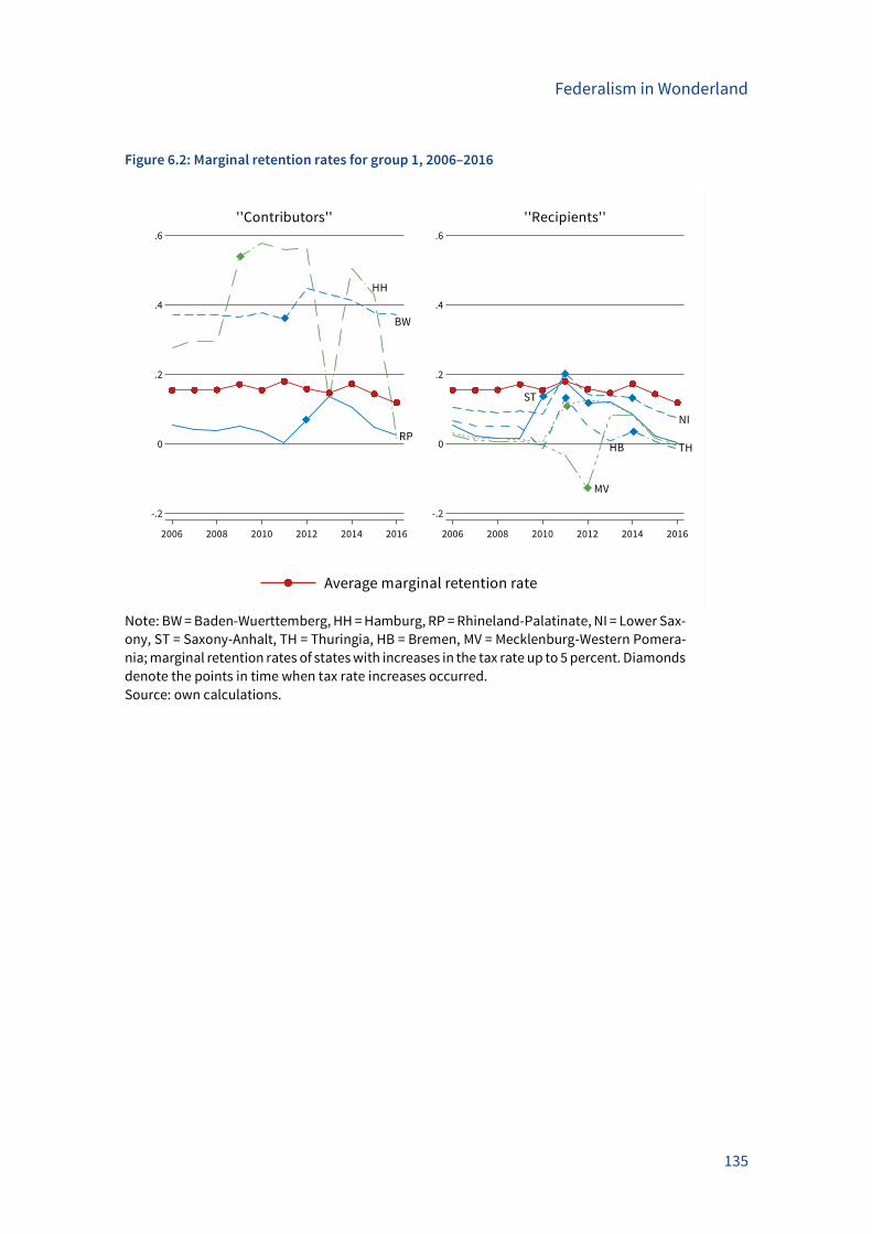
Federalism in Wonderland
135
Figure 6.2: Marginal retention rates for group 1, 2006–2016
Note: BW = Baden-Wuerttemberg, HH = Hamburg, RP = Rhineland-Palatinate, NI = Lower Sax-
ony, ST = Saxony-Anhalt, TH = Thuringia, HB = Bremen, MV = Mecklenburg-Western Pomera-
nia; marginal retention rates of states with increases in the tax rate up to 5 percent. Diamonds
denote the points in time when tax rate increases occurred.
Source: own calculations.
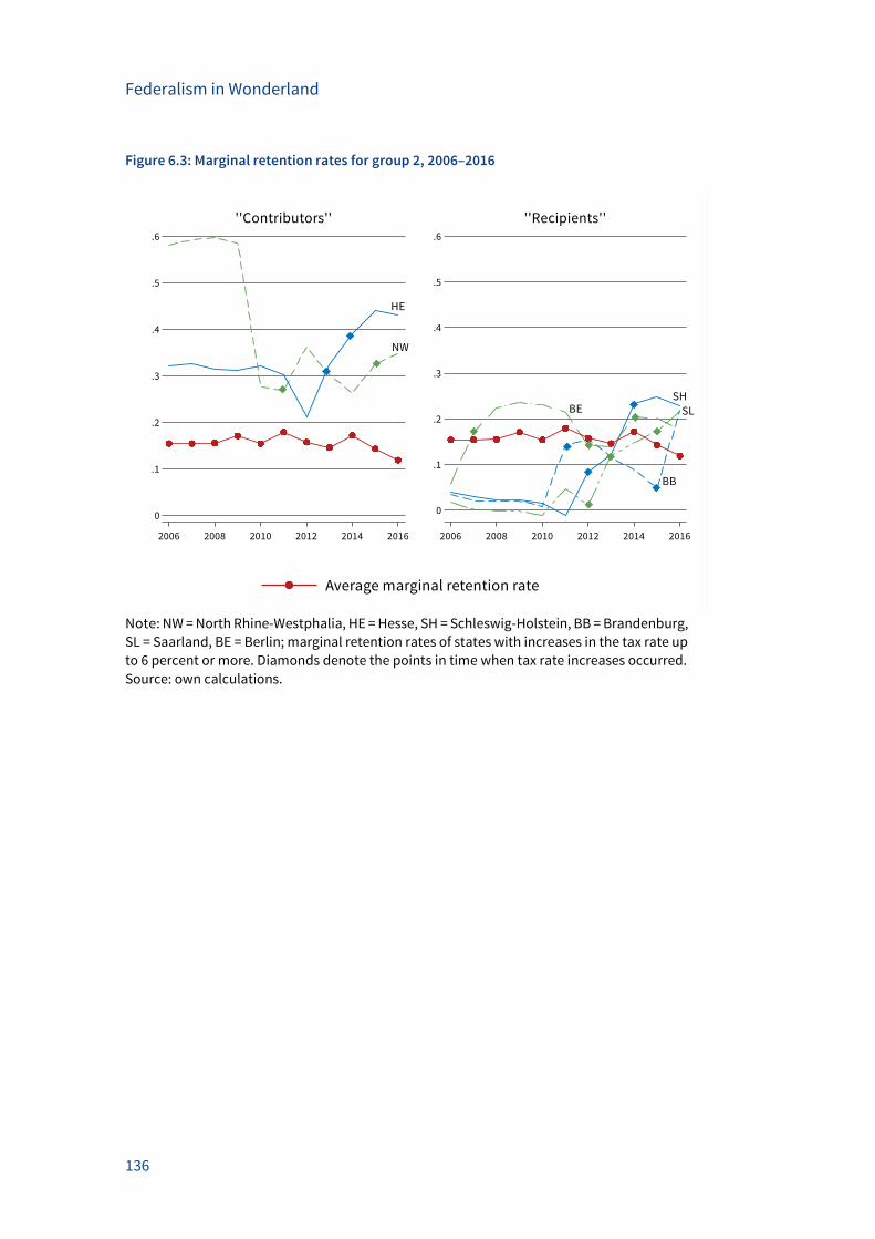
Federalism in Wonderland
136
Figure 6.3: Marginal retention rates for group 2, 2006–2016
Note: NW = North Rhine-Westphalia, HE = Hesse, SH = Schleswig-Holstein, BB = Brandenburg,
SL = Saarland, BE = Berlin; marginal retention rates of states with increases in the tax rate up
to 6 percent or more. Diamonds denote the points in time when tax rate increases occurred.
Source: own calculations.
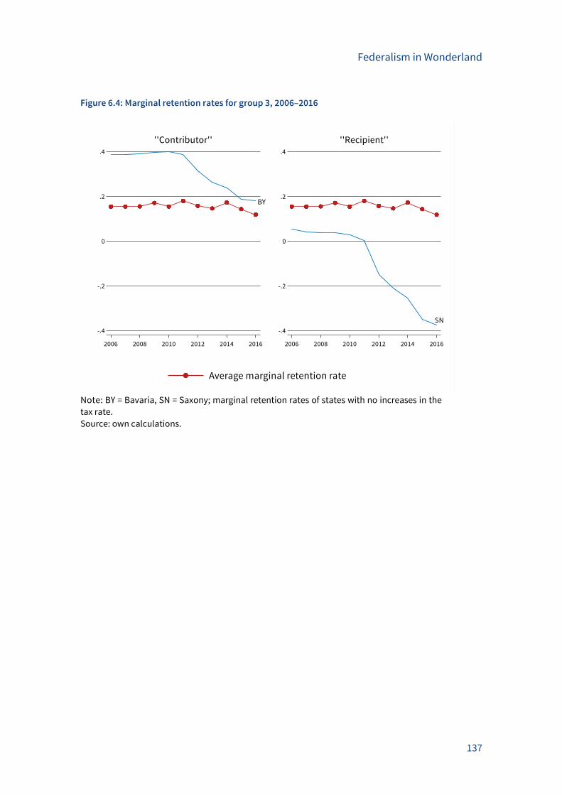
Federalism in Wonderland
137
Figure 6.4: Marginal retention rates for group 3, 2006–2016
Note: BY = Bavaria, SN = Saxony; marginal retention rates of states with no increases in the
tax rate.
Source: own calculations.

Federalism in Wonderland
138
Fiscal equalization as a driver of tax increases
139
7 Fiscal equalization as a driver of tax
increases: Empirical evidence from Germany
Fiscal equalization as a driver of tax increases
Abstract*
This chapter exploits a recent devolution of tax setting powers in the German federation to
study the effects of fiscal equalization on subnational governments’ tax policy. Based on an
analysis of the system of fiscal equalization transfers, we argue that the redistribution of rev-
enues provides incentives for states to raise rather than to lower their tax rates. The empirical
analysis exploits differences in fiscal redistribution among the states and over time. Using a
comprehensive simulation model, we compute the tax-policy incentives faced by each state
over the years and explore their empirical effects on tax policy. The results support significant
and substantial effects. Facing full equalization, a state is predicted to set the tax rate from
the real-estate transfer tax about 1.3 percentage points higher than without. Our analysis also
shows that the incentive to raise tax rates is proliferated by the equalization system because
the states’ decisions to raise their tax rates have intensified fiscal redistribution over time.
* This chapter is based on joint work with Thiess Büttner. We would like to thank Niklas Potrafke, Willem Sas and seminar partic-
ipants on various workshops and conferences for helpful suggestions and comments as well as Tobias Görbert for excellent re-
search assistance.
Fiscal equalization as a driver of tax increases
140
Introduction
A key characteristic of federal public finance is the fiscal autonomy of subnational govern-
ments. This includes the discretion to decide about expenditures and to impose local taxes.
In federations, this autonomy is often combined with equalization transfers ensuring that all
subnational governments have sufficient funding to provide a similar level of public good pro-
vision. As Boadway (2004, p. 212) puts it “...equalization can be seen as necessary counterpart
to decentralization, offsetting its tendency to create disparities among regions in the ability
to provide public goods and services.” However, since fiscal equalization provides jurisdic-
tions with more funds when own revenues decline, fiscal equalization may alter the incentives
of subnational governments to raise own source revenues. In particular, receiving states may
reduce their own tax effort (e.g., Musgrave 1961). Yet, depending on how fiscal equalization is
designed, it may provide incentives to increase rather than lower taxes (e.g., Smart 1998).
In a recent reform, the German federation has aimed to strengthen the autonomy of state
governments in taxation and assigned the tax rate of the real-estate transfer tax (RETT) to the
discretion of the states. The system of fiscal equalization was left basically unchanged, how-
ever. As depicted in Figure 7.1, the reform in 2006 had strong effects on tax policy. In the decade
following the reform, the 16 German states have enacted no less than 26 tax increases – no
state has lowered its tax rate. Initially, the tax rate was 3.5 percent on the sales price. In some
states, the tax rate has almost doubled; in 2017, the mean tax rate has reached a level of 5.4
percent.
The economic literature suggests that the RETT is a rather inefficient tax instrument. Because
the tax drives a wedge between the buyer’s and seller’s price, real-estate transactions are de-
terred and matching efficiency on real estate and labor markets is adversely affected (e.g.,
Lundborg and Skedinger 1999, Adam et al. 2011, Dachis et al. 2012). The fact that the states
have utilized this distortionary tax instrument so heavily may indicate that they are under sub-
stantial revenue stress. As we show in this chapter, an alternative explanation is that, rather
than simply depressing efforts to raise own source revenues, the combination of tax auton-
omy and fiscal equalization in Germany actually provides strong incentives to raise the local
tax rates.
The incentives of subnational governments for tax policy are the subject of a large body of
economic literature (for surveys see Wilson 1999, Keen and Konrad 2013). This literature has
emphasized in particular that tax policy of individual governments exerts fiscal externalities
on others. If the set of tax instruments is restricted, the resulting tax competition equilibrium
is typically characterized by inefficiently low tax rates. The literature has also noted that fed-
eral countries have institutions that work in the opposite direction (Keen and Kotsogiannis
2002). In particular, the literature has pointed to the role of fiscal redistribution (e.g., Smart
1998, Köthenbürger 2002, Bucovetsky and Smart 2006). The focus is on the incentives of a
specific type of fiscal redistribution implemented by the Australian, the Canadian, the German
Fiscal equalization as a driver of tax increases
141
as well as the Swiss federations. These countries feature systems of fiscal capacity equaliza-
tion (FCE), where fiscal transfers are a function of fiscal capacity. The latter is typically defined
as a sum of own source revenues, where tax revenues with local discretion are not directly
included. Rather, revenues from local taxes are standardized to reflect the revenues a state
would have collected if the average tax rate is charged on the actual tax base. With fiscal ca-
pacity equalization, the adverse impact of a high tax rate on the tax base, which reflects the
deadweight loss from taxation, depresses the fiscal capacity of the state. Because this results
in higher equalization transfers, states are subject to an incentive to increase the local tax rate
and tend to disregard the economic cost of taxation.
The empirical literature on the tax policy incentives of fiscal capacity equalization is relatively
scarce. Dahlby and Warren (2003) analyze the effects of fiscal equalization on the incentive of
Australian states and territories to raise taxes and note that states that receive more transfers
when raising taxes actually tend to impose higher taxes. Evidence for Canada is provided by
Smart (2007) who uses an instrumental variable approach to find that tax rates in grant-re-
ceiving provinces are higher and more responsive to the tax rates in other provinces. More
recently, Ferede (2017) considers the effects of equalization on provincial business and per-
sonal income tax rates in Canada. As in Dahlby and Warren (2003), the analysis distinguishes
incentives that work through the effects of tax policies on the provincial tax base as well as
through the effects on the average (representative) tax rate used to determine fiscal capacity.
To identify the effects for grant receiving provinces, Ferede (2017) exploits the discontinuity in
the grant allocation formula. The results show that equalization leads to higher tax rates, in
particular to higher personal income tax rates, mainly through its base effects.
Despite the strong fiscal redistribution present in the German federation, there are no papers
providing evidence on incentive effects exerted on the German states’ tax policy. This is, of
course, the consequence of the lack of tax autonomy that characterized German states before
the recent reform. Baretti et al. (2002) as well as Bönke et al. (2017) explore effects of fiscal
redistribution on tax collection efforts.
Empirical research has also explored effects of redistributive state grants to German munici-
palities (e.g., Buettner 2006, Egger et al. 2010, and Rauch and Hummel 2016). While this re-
search generally supports causal effects on local tax policy, the mechanism behind the policy
response differs from fiscal capacity equalization. As noted by Dahlby and Warren (2003), in
systems of fiscal capacity equalization, the degree of redistribution faced by a jurisdiction is
endogenous to tax policy. More specifically, the incentive to raise taxes is also determined by
the tax policy of other jurisdictions. Therefore, fiscal capacity equalization may exert much
stronger effects on tax policy than the grants to municipalities.
This chapter contributes to the literature on tax policy effects of fiscal equalization by explor-
ing the tax policy of German states after the recent federal reform. By considering the period
following the devolution of tax setting powers, the German case provides ideal conditions to
Fiscal equalization as a driver of tax increases
142
study how the tax policy incentives from equalization affect subnational tax policy and how
the incentives are proliferated through the equalization system. In order to measure the spe-
cific tax policy incentive faced by each state we implement a detailed simulation model of the
equalization system, which comprehensively captures the developments in all states over the
observation period. The model provides measures of the degree of fiscal redistribution and
the fiscal position of each state over time, which enables us to distinguish income effects as-
sociated with equalization from its incentive effects. Since the degree of fiscal redistribution
faced by the individual state partly depends on own tax policy and revenues, we employ in-
strumental variables based on simulations that keep a state’s tax rate and its share of the tax
base at pre-reform levels. Controlling for the fiscal position and the associated income effects,
the results support a significant and substantial effect of fiscal equalization on a state’s tax
policy. According to the estimates, with full equalization states set their tax rates from the
real-estate transfer tax about 1.3 percentage points higher than without. Our analysis also
shows that the incentive to raise tax rates is proliferated by the equalization system as each
state’s decision to raise the tax rate has increased the incentive of other states to raise their
taxes as well.
The following section provides an analysis of tax policy under fiscal equalization. Subse-
quently, in Section 7.3 the empirical methodology is discussed, and in Section 7.4 the data is
described. Section 7.5 presents the results. Section 7.6 concludes.
Tax policy under fiscal equalization
This section provides a stylized analysis of optimal tax policy in the presence of fiscal capacity
equalization (FCE). For simplicity, the revenues 𝑅𝑖 of a state i are assumed to consist of three
components
𝑅𝑖 = 𝑇𝑖 + 𝜏𝑖𝐵𝑖 + 𝑍𝑖 .
One component is revenue from shared taxes 𝑇𝑖, the second component is revenue from the
local tax and the third component is a fiscal transfer.
A capacity-based fiscal equalization scheme defines the transfers using a function of the rela-
tive fiscal position 𝑆𝑖 of a state i
𝑍𝑖 > 0 if 𝑆𝑖 < 1
𝑍𝑖 = 𝑍 (𝑆𝑖), where 𝑍𝑖′ < 0 and 𝑍𝑖 = 0 if 𝑆𝑖 = 1
𝑍𝑖 < 0 if 𝑆𝑖 > 1.
The relative fiscal position is defined as
𝑆𝑖 =𝐶𝑖
1
𝑛∑ 𝐶𝑗
,
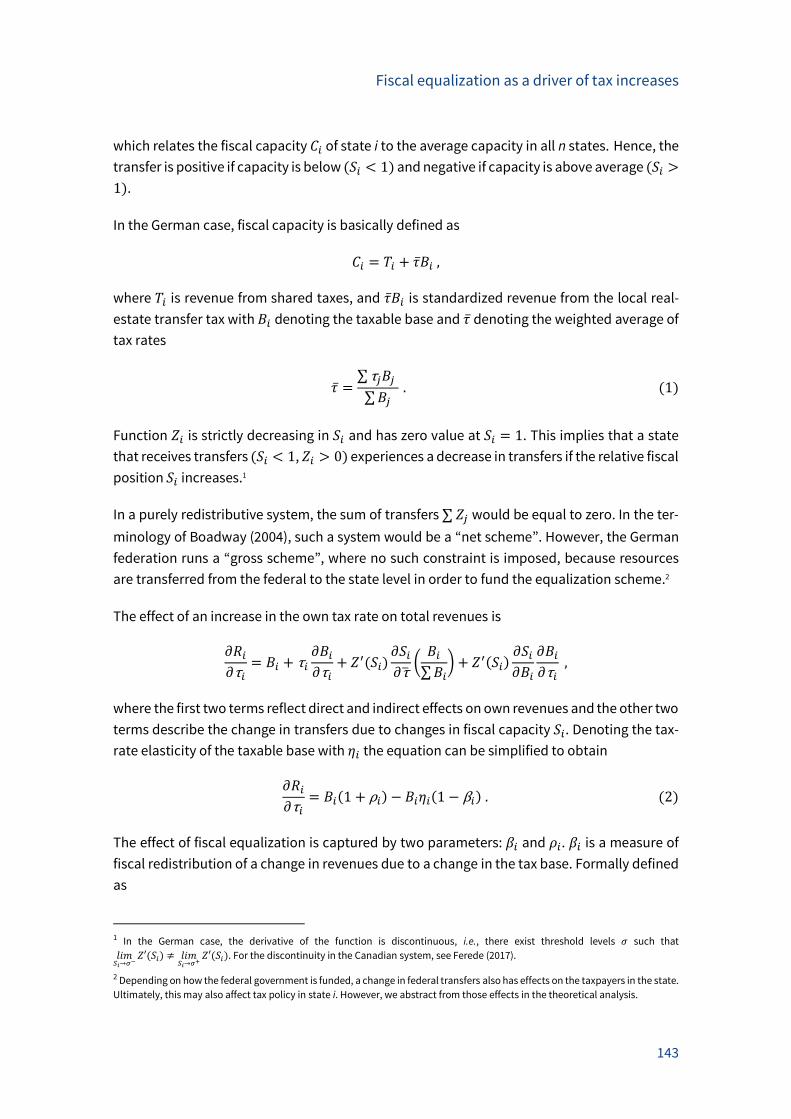
Fiscal equalization as a driver of tax increases
143
which relates the fiscal capacity 𝐶𝑖 of state i to the average capacity in all n states. Hence, the
transfer is positive if capacity is below (𝑆𝑖 < 1) and negative if capacity is above average (𝑆𝑖 >
1).
In the German case, fiscal capacity is basically defined as
𝐶𝑖 = 𝑇𝑖 + �̅�𝐵𝑖 ,
where 𝑇𝑖 is revenue from shared taxes, and �̅�𝐵𝑖 is standardized revenue from the local real-
estate transfer tax with 𝐵𝑖 denoting the taxable base and �̅� denoting the weighted average of
tax rates
�̅� =∑ τ𝑗𝐵𝑗
∑ 𝐵𝑗 . (1)
Function 𝑍𝑖 is strictly decreasing in 𝑆𝑖 and has zero value at 𝑆𝑖 = 1. This implies that a state
that receives transfers (𝑆𝑖 < 1, 𝑍𝑖 > 0) experiences a decrease in transfers if the relative fiscal
position 𝑆𝑖 increases.1
In a purely redistributive system, the sum of transfers ∑ 𝑍𝑗 would be equal to zero. In the ter-
minology of Boadway (2004), such a system would be a “net scheme”. However, the German
federation runs a “gross scheme”, where no such constraint is imposed, because resources
are transferred from the federal to the state level in order to fund the equalization scheme.2
The effect of an increase in the own tax rate on total revenues is
𝜕𝑅𝑖
𝜕τ𝑖= 𝐵𝑖 + τ𝑖
𝜕𝐵𝑖
𝜕τ𝑖+ 𝑍′(𝑆𝑖)
𝜕𝑆𝑖
𝜕τ̅(
𝐵𝑖
∑ 𝐵𝑖) + 𝑍′(𝑆𝑖)
𝜕𝑆𝑖
𝜕𝐵𝑖
𝜕𝐵𝑖
𝜕τ𝑖 ,
where the first two terms reflect direct and indirect effects on own revenues and the other two
terms describe the change in transfers due to changes in fiscal capacity 𝑆𝑖. Denoting the tax-
rate elasticity of the taxable base with 𝜂𝑖 the equation can be simplified to obtain
𝜕𝑅𝑖
𝜕τ𝑖= 𝐵𝑖(1 + ρ𝑖) − 𝐵𝑖𝜂𝑖(1 − β𝑖) . (2)
The effect of fiscal equalization is captured by two parameters: 𝛽𝑖 and 𝜌𝑖. 𝛽𝑖 is a measure of
fiscal redistribution of a change in revenues due to a change in the tax base. Formally defined
as
1 In the German case, the derivative of the function is discontinuous, i.e., there exist threshold levels 𝜎 such that
𝑙𝑖𝑚𝑆𝑖→𝜎−
𝑍′(𝑆𝑖) ≠ 𝑙𝑖𝑚𝑆𝑖→𝜎+
𝑍′(𝑆𝑖). For the discontinuity in the Canadian system, see Ferede (2017).
2 Depending on how the federal government is funded, a change in federal transfers also has effects on the taxpayers in the state.
Ultimately, this may also affect tax policy in state i. However, we abstract from those effects in the theoretical analysis.
Fiscal equalization as a driver of tax increases
144
𝛽𝑖 = – (𝑍′(𝑆𝑖)𝜕𝑆𝑖
𝜕𝐵𝑖τ𝑖⁄ ) > 0 , (3)
it captures the fraction of an increase in revenues due to a higher tax base that is compensated
through transfers. This effect has been dubbed equalization base effect (Dahlby and Warren
2003). Since the relative fiscal position increases with the tax base, –𝑍′(𝑆𝑖) 𝜕𝑆𝑖 𝜕𝐵𝑖⁄ deter-
mines the loss in transfers given an increase in the tax base. Dividing this loss in transfers by
the tax rate relates the change in revenues to the direct revenue effect from an increase in the
tax base. If 𝛽𝑖 is close to zero, a higher tax base has little impact on transfers and the revenue
gain from an increase in the tax base is mainly kept by the state. If 𝛽𝑖 is close to unity, a higher
tax base results in a strong decline in fiscal transfers. In this case, the net revenue impact of
an increase in the tax base is small. If 𝛽𝑖 exceeds unity, a higher tax base would result in net-
revenue losses. While such heavy redistribution seems hard to justify, it cannot be ruled out
for practical applications. If the state is net contributor (𝑍𝑖 < 0), an increase in the tax base is
associated with a higher contribution. In this case 𝛽𝑖 measures the extent to which a revenue
increase due to a higher tax base is compensated by higher contributions.
With regard to the revenue effect of a tax-rate increase in Equation (2), 𝛽𝑖 tends to reduce the
revenue implication of the adverse effect of higher taxes on the tax base. As a consequence,
the higher 𝛽𝑖 the larger is the revenue gain from higher taxes.
The second parameter characterizing fiscal equalization, 𝜌𝑖, is a measure of fiscal redistribu-
tion of a change in revenues due to the tax rate at a given tax base. Dahlby and Warren (2003)
call this the equalization rate effect. Formally defined as
𝜌𝑖 = (𝑍′(𝑆𝑖)𝜕𝑆𝑖
𝜕�̅�(
𝐵𝑖
∑ 𝐵𝑗) 𝐵𝑖⁄ ) , (4)
it captures the fraction of an increase in revenues due to a higher tax rate at a given tax base
that is compensated through transfers. The effect of the local tax rate on the average (repre-
sentative) tax rate at a given tax base is determined by the share in the total tax
base (𝐵𝑖 ∑ 𝐵𝑗⁄ ). Hence, any increase in the tax rate raises the average tax rate. However,
whether this contributes to an increase in the relative fiscal capacity or not depends on the
fraction of the standardized tax revenues in fiscal capacity in state i relative to all other states.3
The parameter 𝜌𝑖 scales the effect on transfers with the actual tax base 𝐵𝑖 in order to relate
the change in revenues from transfers to the “mechanical” revenue effect of an increase in the
tax rate.
3 Note that
𝜕𝑆𝑖
𝜕�̅�= 𝑆𝑖[
𝐵𝑖
𝐶𝑖−
∑ 𝐵𝑗𝑗
∑ 𝐶𝑗𝑗].
If states with low fiscal capacity have also a low share of the tax in total capacity, 𝜕𝑆𝑖 𝜕𝜏̅⁄ < 0. In this case, a state that receives
transfers, would see a decline in its fiscal position when the average tax rate rises 𝜕𝑆𝑖 𝜕𝜏̅⁄ < 0. As this decline triggers more trans-
fers, 𝜌𝑖 would be positive.
Fiscal equalization as a driver of tax increases
145
If 𝜌𝑖 is close to zero, a higher tax rate has little direct impact on transfers and the mechanical
revenue gain from an increase in the tax rate at a given tax base is mainly kept by the state. If
𝜌𝑖 is positive (negative), the net revenue impact of an increase in the tax rate at a given tax
base is larger (smaller) than the mechanical revenue gain. Hence, the revenue effect of a tax
increase in Equation (2) increases with a positive and decreases with a negative 𝜌𝑖.
To discuss the implications of fiscal equalization for tax policy we assume that the incidence
of the RETT is on the local constituency and consider the marginal cost of public funds4
𝑀𝐶𝐹𝑖 = 𝐵𝑖 (𝜕𝑅𝑖
𝜕𝜏𝑖)−1 =
1
(1 + 𝜌𝑖) − 𝜂𝑖(1 − 𝛽𝑖) .
In the absence of fiscal redistribution, 𝛽𝑖 = 0, 𝜌𝑖 = 0, the marginal cost of funds is simply an
increasing function of the elasticity of the tax base. With fiscal redistribution, 𝛽𝑖 > 0 and the
marginal cost of funds is reduced. This provides an incentive to expand public consumption
and to increase tax rates. With 𝛽𝑖 = 1 and 𝜌𝑖 = 0, the marginal cost of funds would be unity.
In this case, the tax would effectively be perceived as a lump-sum tax.5 If 𝛽𝑖 > 1, the marginal
cost of funds may even be smaller than unity. If the equalization rate effect 𝜌𝑖 is positive, the
marginal cost of funds declines. This is intuitive since a tax-rate increase would then weaken
the fiscal position and more fiscal transfers are obtained.
While we have focused on how the equalization transfers that are received or paid by a state
are affected by the choice of the local tax rate of this state, the transfers also depend on the
tax policy decisions in other states. Even if there are no direct tax externalities, such that the
tax base in one state is unaffected by the local tax rate in other states 𝜕𝐵𝑖 𝜕𝜏𝑗⁄ = 0, other
states’ tax policies exert effects: the relative fiscal position and the average tax rate both de-
pend on the tax rates and tax bases in all other states. Hence, the parameters 𝜌𝑖 and 𝛽𝑖 vary
with the tax policies in other states.
Empirical methodology
In the empirical analysis, we consider the states’ tax policies after a federal reform that
granted the states the right to set the tax rate of the real-estate transfer tax (RETT). The anal-
ysis exploits the fact that the degree of fiscal redistribution differs among the states and over
time.
4 Note that we discuss the marginal cost of public funds from the perspective of a state government. The perspective of the fed-
eration might be different, see Wildasin (1989).
5 Bucovetsky and Smart (2006) show that with full equalization 𝛽𝑖 = 1, the incentive to engage in horizontal tax competition is
eliminated.
Fiscal equalization as a driver of tax increases
146
The empirical analysis focuses on the choice of the RETT rate. Basically, it is concerned with
the relationship between the tax rate and precise indicators of fiscal equalization. This in-
cludes the degree of fiscal redistribution associated with the tax base 𝛽𝑖 and with the tax rate
𝜌𝑖. Based on the theoretical discussion, we assume that if the degree of fiscal redistribution is
high, a state is more likely to increase its tax rate. Since the tax policy is required to set the tax
rate in advance, state governments base their tax decisions for the upcoming period on the
realization of fiscal capacity and on the realized degree of fiscal redistribution.6 This suggests
to use the following specification
Δ𝜏𝑖,𝑡+1 = 𝛼𝑖 + 𝑏1𝛽𝑖,𝑡 + 𝑏2𝜌𝑖,𝑡 + ∑ 𝑏3,𝑗𝑆𝑖,𝑡𝑝
+ 𝛾𝑡
𝑝
𝑗=1
+ 𝜀𝑖,𝑡 (5)
where 𝛼𝑖 is a fixed state effect and 𝛾𝑡 is a fixed time effect for period t. The latter captures
common trends in the German federation. 𝑏1 and 𝑏2 capture the effects of fiscal redistribu-
tion. In the light of the above analysis, positive coefficients are expected as the marginal cost
of funds is reduced when 𝛽𝑖 and 𝜌𝑖 increase.
The identification strategy utilizes the fact that the equalization transfers are formula based
and are determined by a smooth function of relative fiscal capacity. By allowing for arbitrary
non-linear effects of the assignment variable 𝑆𝑖,𝑡𝑝
, the estimation approach ensures that only
differences in the degree of fiscal redistribution conditional on the fiscal position of a state are
used to identify the incentive effects of fiscal equalization. Thereby, we make sure that the
variation in the degree of fiscal redistribution is not capturing differences in available re-
sources and in the amount of equalization transfers. This is important, since the fiscal equali-
zation transfers received, or paid, exert income effects on tax policy. Without controls for rel-
ative fiscal capacity, empirical responses to the indicators of the degree of fiscal redistribution
would capture not only the incentive but also these income effects. To allow for slow adjust-
ment in tax policy, we also provide results of specifications that condition on the current tax
rate.7
As shown above, the degree of fiscal redistribution of RETT revenues is partly determined by
local tax policies. To avoid potential biases, we employ instrumental variables. The instru-
ments used are measures of degree of fiscal redistribution �̂�𝑖,𝑡 and �̂�𝑖,𝑡 faced by state i in pe-
riod t computed by counterfactual simulations, i.e., based on simulations that keep a state’s
6 The first preliminary account of equalization transfers for a budget year is typically published by the Federal Ministry of Finance
in January of the next year. Detailed revenue forecasts for the current budget year are available not before November when the
federal forecast of tax revenues for the current year is issued.
7 Since the dimension of the data covers a limited time period, accurate estimations of the adjustment speed may be difficult due
to the Nickell (1981) bias. Since also the cross-sectional dimension is limited, however, we decided against using GMM methods
that rely on large n asymptotics.
Fiscal equalization as a driver of tax increases
147
tax rate and share of the tax base at pre-reform levels. In other words, as instrumental varia-
bles we use indicators of the degree of fiscal redistribution that a state would face if it had not
used its newly assigned discretion to set the tax rate and, thus, has kept the tax rate at the
pre-reform level. To this end, we fix the state i ’s tax rate at the pre-reform level. Moreover, to
avoid capturing indirect tax policy effects on the tax base we also fix the state’s share in the
total tax base 𝐵𝑖 ∑ 𝐵𝑗⁄ at the pre-reform level of the year 2006. Thus, the variation in the indi-
cators used as instrumental variables derives from changes in the fiscal equalization system
independent of the tax policy in the respective state. Since we condition on the relative fiscal
capacity 𝑆𝑖,𝑡𝑝
, income effects from fiscal equalization are captured, and the instrumental vari-
able should not exert any separate influence on tax policy, i.e., the exclusion restriction of the
instrumental variable is unlikely to be violated.
Data
The empirical analysis examines the choice of the tax rate under fiscal capacity equalization.
It explores how German states responded with their tax rates after they received the right to
set the tax rate of the RETT and, in particular, whether the tax policy response differs depend-
ing on the tax policy incentives associated with fiscal capacity equalization as discussed in
Section 7.2. The analysis explores the tax policy decisions of the states in the period from 2007
to 2017.8 To identify differences in fiscal equalization we exploit the institutional details of fis-
cal equalization among German states. Therefore, the next subsection provides a brief discus-
sion of fiscal equalization. Subsequently, descriptive statistics on tax rates and indicators of
tax policy incentives are provided.
7.4.1 Fiscal equalization in Germany
The German system of fiscal equalization consists of different stages of vertical and horizontal
distribution of funds. The first stage involves the distribution of VAT revenue shared between
the federal and the state governments. The states’ share is distributed mainly according to
population size but a fraction is used to provide funds to states with low fiscal capacity, i.e.,
to states with own tax revenues below average. At this stage, fiscal capacity is calculated with-
out VAT revenues. The second stage consists of a horizontal redistribution scheme with trans-
fers paid to states with fiscal capacity (including VAT) below fiscal need and contributions
made by states with fiscal capacity above fiscal need. The latter is the population-weighted
average of fiscal capacity across states. The third stage uses the same measure of fiscal ca-
pacity and provides further vertical transfers by the federal government to states with fiscal
capacity below fiscal need.
8 The observation period covers 26 tax-rate changes. In 2018, no state has changed the tax rate.
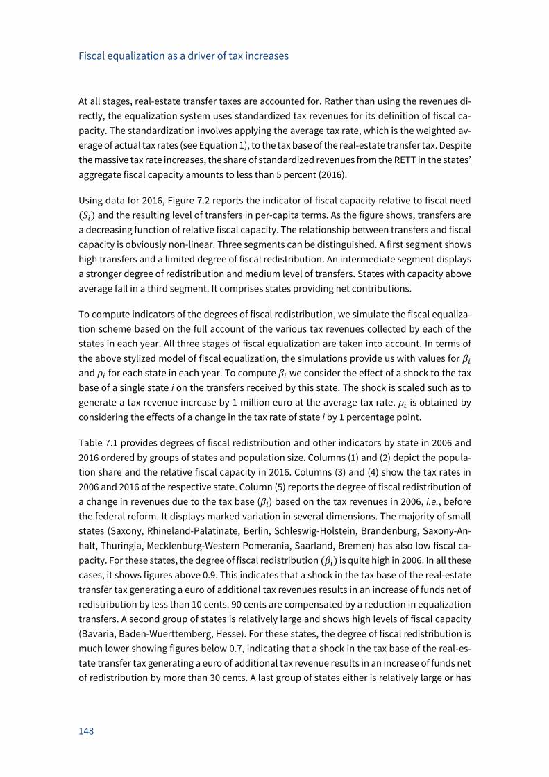
Fiscal equalization as a driver of tax increases
148
At all stages, real-estate transfer taxes are accounted for. Rather than using the revenues di-
rectly, the equalization system uses standardized tax revenues for its definition of fiscal ca-
pacity. The standardization involves applying the average tax rate, which is the weighted av-
erage of actual tax rates (see Equation 1), to the tax base of the real-estate transfer tax. Despite
the massive tax rate increases, the share of standardized revenues from the RETT in the states’
aggregate fiscal capacity amounts to less than 5 percent (2016).
Using data for 2016, Figure 7.2 reports the indicator of fiscal capacity relative to fiscal need
(𝑆𝑖) and the resulting level of transfers in per-capita terms. As the figure shows, transfers are
a decreasing function of relative fiscal capacity. The relationship between transfers and fiscal
capacity is obviously non-linear. Three segments can be distinguished. A first segment shows
high transfers and a limited degree of fiscal redistribution. An intermediate segment displays
a stronger degree of redistribution and medium level of transfers. States with capacity above
average fall in a third segment. It comprises states providing net contributions.
To compute indicators of the degrees of fiscal redistribution, we simulate the fiscal equaliza-
tion scheme based on the full account of the various tax revenues collected by each of the
states in each year. All three stages of fiscal equalization are taken into account. In terms of
the above stylized model of fiscal equalization, the simulations provide us with values for 𝛽𝑖
and 𝜌𝑖 for each state in each year. To compute 𝛽𝑖 we consider the effect of a shock to the tax
base of a single state i on the transfers received by this state. The shock is scaled such as to
generate a tax revenue increase by 1 million euro at the average tax rate. 𝜌𝑖 is obtained by
considering the effects of a change in the tax rate of state i by 1 percentage point.
Table 7.1 provides degrees of fiscal redistribution and other indicators by state in 2006 and
2016 ordered by groups of states and population size. Columns (1) and (2) depict the popula-
tion share and the relative fiscal capacity in 2016. Columns (3) and (4) show the tax rates in
2006 and 2016 of the respective state. Column (5) reports the degree of fiscal redistribution of
a change in revenues due to the tax base (𝛽𝑖) based on the tax revenues in 2006, i.e., before
the federal reform. It displays marked variation in several dimensions. The majority of small
states (Saxony, Rhineland-Palatinate, Berlin, Schleswig-Holstein, Brandenburg, Saxony-An-
halt, Thuringia, Mecklenburg-Western Pomerania, Saarland, Bremen) has also low fiscal ca-
pacity. For these states, the degree of fiscal redistribution (𝛽𝑖) is quite high in 2006. In all these
cases, it shows figures above 0.9. This indicates that a shock in the tax base of the real-estate
transfer tax generating a euro of additional tax revenues results in an increase of funds net of
redistribution by less than 10 cents. 90 cents are compensated by a reduction in equalization
transfers. A second group of states is relatively large and shows high levels of fiscal capacity
(Bavaria, Baden-Wuerttemberg, Hesse). For these states, the degree of fiscal redistribution is
much lower showing figures below 0.7, indicating that a shock in the tax base of the real-es-
tate transfer tax generating a euro of additional tax revenue results in an increase of funds net
of redistribution by more than 30 cents. A last group of states either is relatively large or has
Fiscal equalization as a driver of tax increases
149
large fiscal capacity (North Rhine-Westphalia, Lower Saxony, Hamburg). Here the degree of
fiscal redistribution varies but is lower than for the first group.
The figures for 2016 look very different (see Column 6). Though the system of fiscal equaliza-
tion is the same, for some states 𝛽𝑖 has increased, for others it has declined. It seems that the
changes are mainly the consequence of changes in tax rates. States that have increased their
tax rate the most, such as Berlin, Brandenburg and Saarland, face a decline in fiscal redistri-
bution relative to 2006. The two states that have not increased their tax rate experience an
increase in the degree of fiscal redistribution (Saxony and Bavaria). Most notably in Saxony
the degree of fiscal redistribution is above 1 in 2016. With a degree of fiscal redistribution of
about 1.40, the state loses transfers for each euro of additional tax revenues in an amount of
1.40 euro. Hence, at the margin, the state’s revenues decline by 40 cents with every additional
euro of revenues from the real-estate transfer tax. This extreme level of redistribution9 is not
observed for any other state in 2016. However, Bremen and Mecklenburg-Western Pomerania
also show degrees of fiscal redistribution above 1.
Columns (7) and (8) report the degree of fiscal redistribution of a change in revenues due to
the tax rate (given the tax base) (𝜌𝑖) based on data for 2006 and 2016. It shows little variation
and is in most cases very close to zero. This indicates that the fiscal redistribution of the me-
chanical revenue effects from a tax rate change is very small. Hence, the equalization rate ef-
fect is unimportant in the case of the German RETT.
Figure 7.3 depicts the evolution of the degree of fiscal redistribution of tax base effects over
time. The figure reports the actual degree of fiscal redistribution of revenue effects of a shock
in the tax base. Accordingly, in 2006 the degree of redistribution of a tax-base shock varies
between 0.4 and 1. The mean and the variance of the degree of fiscal redistribution tend to
increase over time.
While the actual degree of redistribution is affected by the own choice of the tax rate, Figure
7.4 reports the development based on the counterfactual simulations. These simulations are
based on the assumption that the tax rate and the share in the tax base of the state under
consideration have stayed constant at the pre-reform level. The distribution shows less fluc-
tuations, but the degree of fiscal redistribution shows a clear positive trend for all states. Dur-
ing the observation period, if a state had not changed its tax rate, the degree of fiscal redistri-
bution of tax base effects for this state has, on average, grown by about a third.
7.4.2 Descriptive statistics
Table 7.2 provides descriptive statistics for the tax rates and the two key variables of interest,
i.e., the degrees of fiscal redistribution with regard to the tax base and the tax rate, as well as
9 The fact that there is more than 100 percent redistribution has been noted in the German debate, see, for instance, Boysen-
Hogrefe (2017) and Buettner and Krause (2018) – see also Chapter 6.
Fiscal equalization as a driver of tax increases
150
for control variables. The latter group includes the indicator of relative fiscal capacity and the
population size. The table also includes indicators for the relative fiscal capacity excluding
VAT, which is used in the first stage of fiscal equalization. It is included in the subsequent anal-
ysis since the first stage of the equalization scheme exerts separate income effects.
Results
Results from a basic set of OLS regressions are provided in Table 7.3. Given the very small
degree of redistribution of revenue effects from tax rate changes (𝜌𝑖), it focuses on the redis-
tribution of the tax base. The first specification includes only the degree of fiscal redistribution
(𝛽𝑖). It shows a significant positive effect. The next three specifications include indicators of
the assignment variable, i.e., of relative fiscal capacity. Even though the higher-order terms
improve the fit of the regression, the degree of fiscal redistribution exerts a similar effect on
the tax policy. According to specifications (5) to (7) the positive effect of fiscal redistribution is
robust against inclusion of relative fiscal capacity excluding VAT – an indicator that captures
assignment in the first stage of equalization. In order to allow for some adjustment in the tax
rate in the first years after the devolution of the right to set the own tax rate, Column (8) adds
the current level of the tax rate. Hence, this specification considers tax policy for the upcoming
period, conditional on the current choice of the tax rate. With this control added, the degree
of fiscal redistribution is still found to exert a significant positive effect, but the effect turns
out to be smaller. This supports the view that the effect of the actual degree of fiscal redistri-
bution is confounded by the current tax policy.
Results from IV estimates are provided in Table 7.4. The estimations employ a measure of the
degree of fiscal redistribution (�̂�𝑖) as an instrumental variable that is based on counterfactual
simulations. It captures the degree of redistribution faced by the state if its tax rate and its
share of the tax base had stayed unchanged at the pre-reform level. For all specifications, the
first stage F-statistic for the excluded instrument provided at the bottom of the table indicates
that the counterfactual simulation provides a strong predictor of the actual degree of fiscal
redistribution. Compared with the OLS results, the results point to somewhat smaller effects
of fiscal redistribution on tax policy.
Quantitatively, the point estimate provided by Column (7) suggests that in presence of full
fiscal redistribution of tax-base shocks (𝛽 = 1) the tax rate is by about 1.3 percentage points
higher compared with a hypothetical situation, where fiscal redistribution is absent (𝛽 = 0).
The analysis has focused on the redistribution of tax base effects. Table 7.5 provides results
of specifications that also include the indicator of the degree of fiscal redistribution associ-
ated with the tax rate effect. While the above findings are confirmed, no significant effect is
found for this second indicator.
Fiscal equalization as a driver of tax increases
151
Since the estimations condition on the fiscal position of a state, the effect found for fiscal re-
distribution suggests that the remarkable series of tax increases after the reform in 2006 can-
not be explained simply with lack of funds but results from the incentive effect of fiscal redis-
tribution. To test whether fiscal distress associated with the level of public debt may partly
explain the tax policy, we have conducted robustness checks where the level of public debt
per capita is added as a control (see Table 7.6). Even though per-capita debt shows a small
positive effect, it does not turn out to be statistically significant and the estimates of the effect
of fiscal redistribution show qualitatively similar effects as above.
Summary and conclusions
This chapter has explored the German states’ tax policy response to a recent reform, which
involves the devolution of tax setting powers to the German states. More specifically, starting
in 2007 German states used the right to choose the tax rate of the real-estate transfer tax. This
reform resulted in an unprecedented wave of tax increases. In the time period from 2007 to
2017 among the 16 German states, no less than 26 tax increases occurred. No state has low-
ered its tax rate. Initially, the tax rate was 3.5 percent on the sales price. In 2017, the mean tax
rate is 5.4 percent.
As we argue in this chapter, due to a system of fiscal capacity equalization, the German states’
tax policy is subject to strong incentives to increase the tax rates of the real-estate transfer
tax. Following Dahlby and Warren (2003), we identify two separate incentives for tax policy.
The first incentive is associated with the effect of the tax rate on the tax base. Given the way
fiscal capacity is defined, the adverse impact of a high tax rate on the tax base, which reflects
the deadweight loss from taxation, contributes to a decline in fiscal capacity. Hence, a state
that raises its tax rate, receives more rather than less equalization transfers or, if it is a state
with high fiscal capacity, needs to make lower transfers to other states. A second incentive
effect can arise, since each state’s tax policy decision is reflected in the average tax rate that
is used by the equalization system to determine fiscal capacity.
To test whether these incentive effects have led the states to increase their tax rate in the re-
cent years, we use a simulation analysis of the system of fiscal equalization and precisely com-
pute the incentives faced by each state in each period. The identification strategy exploits dif-
ferences in the degree of fiscal redistribution among the states and over time. To distill the
incentive effects empirically, we comprehensively control for income effects of fiscal redistri-
bution by indicators of the relative fiscal capacity. To overcome possible confounding effects
of own policies on the incentive effect we use an instrumental variables approach. More spe-
cifically, by means of counterfactual simulations we compute indicators of the degree of fiscal
redistribution that keep a state’s tax rate and its share of the tax base at pre-reform levels,
which are used as instrumental variables.
Fiscal equalization as a driver of tax increases
152
The results support a robust significant effect of fiscal redistribution on tax policy. According
to the point estimates, with full equalization of tax revenues, the tax rate for the real-estate
transfer tax is about 1.3 percentage points higher than without. This sizeable incentive effect
is exclusively associated with the fiscal redistribution of the tax base. The equalization rate
effect is unimportant in the German context.
Given that the German states were mostly subject to almost full equalization when the reform
was implemented, the incentive provided by tax base equalization can explain a substantial
part of the recent tax increases by German states. In addition, however, the basic incentive
effect to raise the own tax rate has been proliferated by the equalization system. As states
responded to the tax policy incentive by setting higher tax rates, the strength of the incentive
faced by a state has been increasing over time. Hence, the first wave of tax increases raised
the incentive to increase tax rates and triggered further tax increases.
Our findings point to the importance of a careful design of federal fiscal institutions. Combin-
ing a high degree of fiscal redistribution with a decentralized distortionary tax likely results in
an inefficient tax structure.
Fiscal equalization as a driver of tax increases
153
References
Adam, S., T. Besley, R. Blundell, S. Bond, R. Chote, M. Gammie, P. Johnson, G. Myles, and J. M.
Poterba (2011). Tax by Design – The Mirrlees Review. Oxford: Oxford University Press.
Baretti, C., B. Huber, and K. Lichtblau (2002). A tax on tax revenue: The incentive effects of
equalizing transfers: Evidence from Germany. International Tax and Public Finance, 9(6),
631–649.
Boadway, R. (2004). The theory and practice of equalization. CESifo Economic Studies, 50(1),
211–254.
Bönke, T., B. Joachimsen, and C. Schröder (2017). Fiscal federalism and tax enforcement. Ger-
man Economic Review, 18, 377–409.
Boysen-Hogrefe, J. (2017). Grunderwerbsteuer im Länderfinanzausgleich: Umverteilung der
Zusatzlast der Besteuerung. Wirtschaftsdienst, 97(5), 354–359.
Bucovetsky, S. and M. Smart (2006). The efficiency consequences of local revenue equaliza-
tion: Tax competition and tax distortions. Journal of Public Economic Theory, 8(1), 119–
144.
Buettner, T. (2006). The incentive effect of fiscal equalization transfers on tax policy. Journal
of Public Economics, 90(3), 477–497.
Buettner, T. and M. Krause (2018). Föderalismus im Wunderland: Zur Steuerautonomie bei der
Grunderwerbsteuer. Perspektiven der Wirtschaftspolitik, 19(1), 32–41.
Dachis, B., G. Duranton, and M. A. Turner (2012). The effects of land transfer taxes on real es-
tate markets: Evidence from a natural experiment in Toronto. Journal of Economic Ge-
ography, 12, 327–354.
Dahlby, B. and N. Warren (2003). Fiscal incentive effects of the Australian equalisation system.
Economic Record, 79, 434–445.
Egger, P., M. Köthenbürger, and M. Smart (2010). Do fiscal transfers alleviate business tax com-
petition? Evidence from Germany. Journal of Public Economics, 94(3), 235–246.
Ferede, E. (2017). The incentive effects of equalization grants on tax policy: Evidence from Ca-
nadian provinces. Public Finance Review, 45(6), 723–747.
Keen, M. and K. A. Konrad (2013). The theory of international tax competition and coordina-
tion. Handbook of Public Economics, 5, 257–297.
Keen, M. J. and C. Kotsogiannis (2002). Does federalism lead to excessively high taxes? Ameri-
can Economic Review, 92(1), 363–370.
Köthenbürger, M. (2002). Tax competition and fiscal equalization. International Tax and Public
Finance, 9(4), 391–408.
Fiscal equalization as a driver of tax increases
154
Lundborg, P. and P. Skedinger (1999). Transaction taxes in a search model of the housing mar-
ket. Journal of Urban Economics, 45, 385–399.
Musgrave, R. A. (1961). Approaches to a fiscal theory of political federalism. In: Public Finances:
Needs, Sources, and Utilization. Princeton: Princeton University Press, pp. 97–134.
Nickell, S. (1981). Biases in dynamic models with fixed effects. Econometrica, 49(6), 1417–1426.
Rauch, A. and C. A. Hummel (2016). How to stop the race to the bottom. International Tax and
Public Finance, 23(5), 911–933.
Smart, M. (1998). Taxation and deadweight loss in a system of intergovernmental transfers.
Canadian Journal of Economics, 31(1), 189–206.
Smart, M. (2007). Raising taxes through equalization. Canadian Journal of Economics, 40(4),
1188–1212.
Wildasin, D. E. (1989). Interjurisdictional capital mobility: Fiscal externality and a corrective
subsidy. Journal of Urban Economics, 25, 193–212.
Wilson, J. D. (1999). Theories of tax competition. National Tax Journal, 52, 269–304.
Fiscal equalization as a driver of tax increases
155
Appendix
A Data sources and definitions
Population size: the population size is the total amount of population in each state on June
30 of each year. Source: Federal Ministry of Finance (Annual announcements of the fiscal
equalization account, (Zweite Verordnung zur Durchführung des Finanzausgleichsgesetzes,
various years)).
Tax rate of the real-estate transfer tax (in percent): the tax rate is the rate of the real-estate
transfer tax in percent applicable to land transactions. In cases where the tax rate has been
changed within a year, the annual figure is interpolated based on the exact calendar days.
Source: announcements of the 16 German states.
Tax base of the real-estate transfer tax (in 1,000 euro): the tax base of the real-estate trans-
fer tax is basically the sale price of the property. Source: Federal Ministry of Finance (Annual
announcements of the fiscal equalization account, (Zweite Verordnung zur Durchführung des
Finanzausgleichsgesetzes, various years)).
Relative fiscal capacity: relative fiscal capacity is defined as fiscal capacity relative to fiscal
need for each state. Fiscal capacity is defined as available revenues including state’s own tax
revenues, the share of income taxes, the VAT share and municipal tax revenues. Fiscal need is
the population weighted average of fiscal capacity across states. Source: Federal Ministry of
Finance (Annual announcements of the fiscal equalization account, (Zweite Verordnung zur
Durchführung des Finanzausgleichsgesetzes, various years)) and own calculations.
Relative fiscal capacity (excl. VAT): relative fiscal capacity excluding revenues from VAT as
used in the first stage of the equalization system to determine the VAT distribution. Source:
Federal Ministry of Finance (Annual announcements of the fiscal equalization account,
(Zweite Verordnung zur Durchführung des Finanzausgleichsgesetzes, various years)) and own
calculations.
Degree of fiscal redistribution (tax base 𝛽): the degree of fiscal redistribution captures the
fraction of an increase in revenues due to a higher tax base that is compensated through trans-
fers. The state-specific shock in the tax base of the RETT is scaled such as to generate a tax
revenue increase by 1 million euro at the average tax rate in all states and periods. Source:
own simulation analysis.
Degree of fiscal redistribution (tax rate 𝜌): the degree of fiscal redistribution captures the
fraction of an increase in revenues due to a higher tax rate (at a given tax base) that is com-
pensated through transfers. The state-specific shock in the tax rate of the RETT is an increase
by 1 percentage point. Source: own simulation analysis.
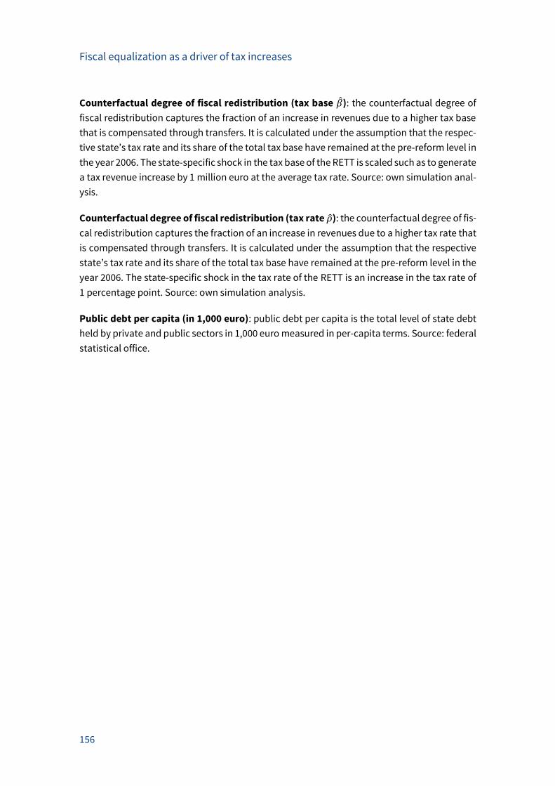
Fiscal equalization as a driver of tax increases
156
Counterfactual degree of fiscal redistribution (tax base �̂�): the counterfactual degree of
fiscal redistribution captures the fraction of an increase in revenues due to a higher tax base
that is compensated through transfers. It is calculated under the assumption that the respec-
tive state’s tax rate and its share of the total tax base have remained at the pre-reform level in
the year 2006. The state-specific shock in the tax base of the RETT is scaled such as to generate
a tax revenue increase by 1 million euro at the average tax rate. Source: own simulation anal-
ysis.
Counterfactual degree of fiscal redistribution (tax rate �̂�): the counterfactual degree of fis-
cal redistribution captures the fraction of an increase in revenues due to a higher tax rate that
is compensated through transfers. It is calculated under the assumption that the respective
state’s tax rate and its share of the total tax base have remained at the pre-reform level in the
year 2006. The state-specific shock in the tax rate of the RETT is an increase in the tax rate of
1 percentage point. Source: own simulation analysis.
Public debt per capita (in 1,000 euro): public debt per capita is the total level of state debt
held by private and public sectors in 1,000 euro measured in per-capita terms. Source: federal
statistical office.
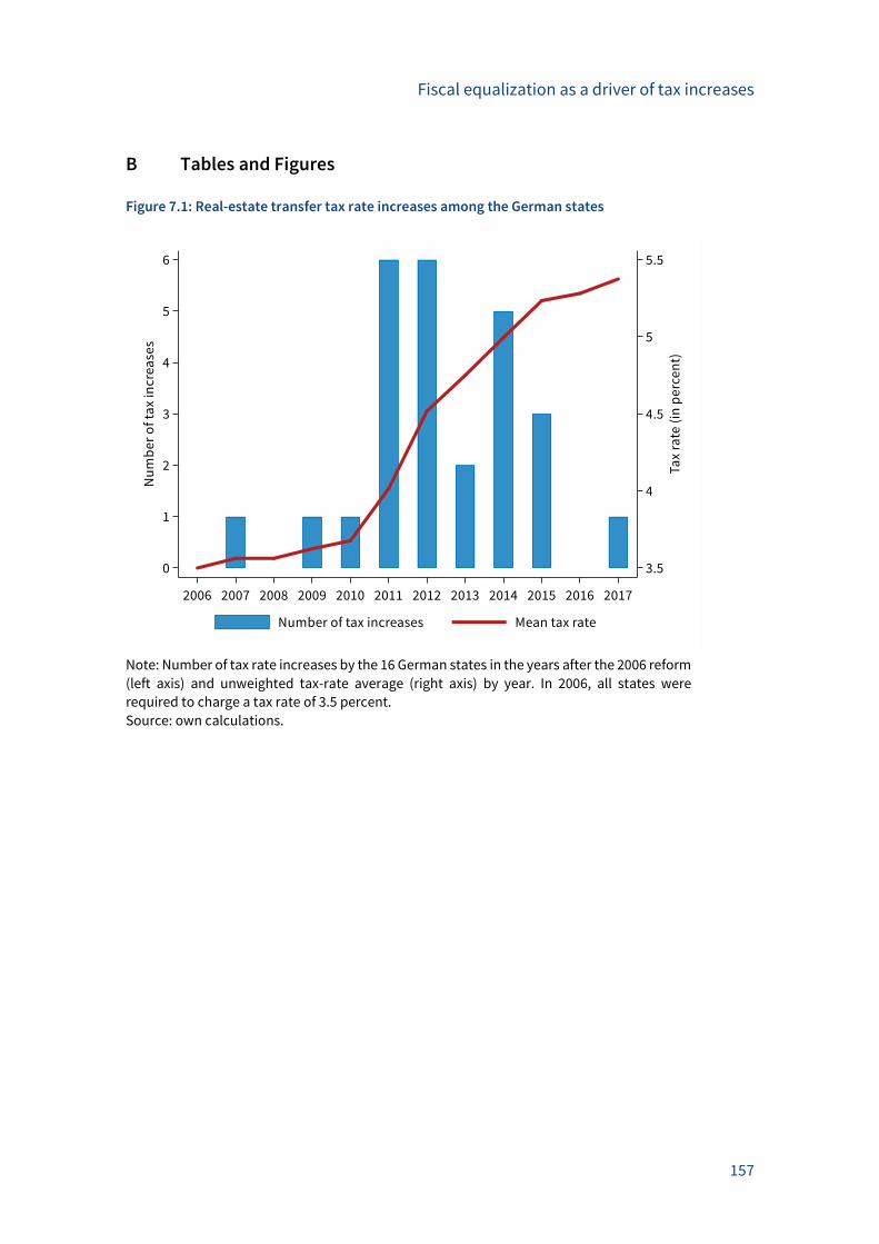
Fiscal equalization as a driver of tax increases
157
B Tables and Figures
Figure 7.1: Real-estate transfer tax rate increases among the German states
Note: Number of tax rate increases by the 16 German states in the years after the 2006 reform
(left axis) and unweighted tax-rate average (right axis) by year. In 2006, all states were
required to charge a tax rate of 3.5 percent.
Source: own calculations.
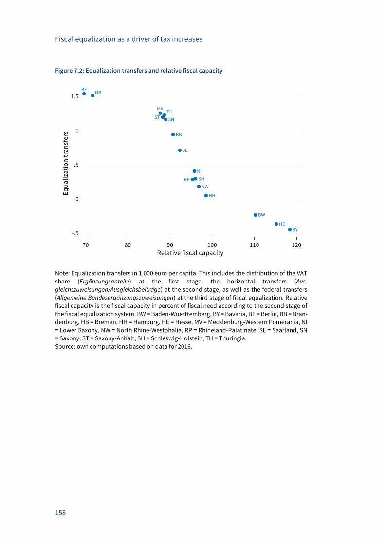
Fiscal equalization as a driver of tax increases
158
Figure 7.2: Equalization transfers and relative fiscal capacity
Note: Equalization transfers in 1,000 euro per capita. This includes the distribution of the VAT
share (Ergänzungsanteile) at the first stage, the horizontal transfers (Aus-
gleichszuweisungen/Ausgleichsbeiträge) at the second stage, as well as the federal transfers
(Allgemeine Bundesergänzungszuweisungen) at the third stage of fiscal equalization. Relative
fiscal capacity is the fiscal capacity in percent of fiscal need according to the second stage of
the fiscal equalization system. BW = Baden-Wuerttemberg, BY = Bavaria, BE = Berlin, BB = Bran-
denburg, HB = Bremen, HH = Hamburg, HE = Hesse, MV = Mecklenburg-Western Pomerania, NI
= Lower Saxony, NW = North Rhine-Westphalia, RP = Rhineland-Palatinate, SL = Saarland, SN
= Saxony, ST = Saxony-Anhalt, SH = Schleswig-Holstein, TH = Thuringia.
Source: own computations based on data for 2016.
Fiscal equalization as a driver of tax increases
159
Table 7.1: Fiscal redistribution by state in 2006 and 2016
Fiscal equalization
Popul.
share
Rel. fiscal
capacity (𝑆𝑖)
Tax rate (𝜏𝑖)
Base effect (𝛽𝑖)
Rate effect (𝜌𝑖)
Year 2016 2016 2006 2016 2006 2016 2006 2016
State (1) (2) (3) (4) (5) (6) (7) (8)
Saxony 4.97 88.95 3.5 3.5 0.95 1.40 -0.02 -0.01
Rhineland-Palatinate 4.93 95.33 3.5 5.0 0.95 0.98 -0.01 -0.01
Berlin 4.28 69.62 3.5 6.0 0.94 0.81 0.03 0.02
Schleswig-Holstein 3.48 96.05 3.5 6.5 0.96 0.76 0.01 0.00
Brandenburg 3.02 90.74 3.5 6.5 0.97 0.78 -0.01 -0.01
Saxony-Anhalt 2.73 88.26 3.5 5.0 0.95 1.00 -0.01 -0.01
Thuringia 2.64 88.64 3.5 5.0 0.97 1.00 -0.02 -0.02
Mecklenburg-Western
Pomerania
1.96 87.67 3.5 5.0 0.98 1.01 -0.01 -0.00
Saarland 1.21 92.29 3.5 6.5 0.98 0.78 -0.00 -0.00
Bremen 0.82 71.65 3.5 5.0 0.93 1.02 -0.00 -0.00
Bavaria 15.63 118.39 3.5 3.5 0.61 0.86 0.01 0.04
Baden-Wuerttemberg 13.24 110.25 3.5 5.0 0.63 0.63 0.00 0.00
Hesse 7.52 115.21 3.5 6.0 0.68 0.56 0.02 0.01
North Rhine-Westphalia 21.74 96.81 3.5 6.5 0.42 0.62 0.01 -0.02
Lower Saxony 9.65 95.75 3.5 5.0 0.89 0.93 -0.02 -0.02
Hamburg 2.18 98.54 3.5 4.5 0.72 0.99 0.01 0.01
Note: Population share and fiscal position (relative fiscal capacity) in percent obtained from the an-
nouncements of the fiscal equalization account of the Federal Ministry of Finance. Relative fiscal ca-
pacity defined as fiscal capacity (Finanzkraftmesszahl) relative to fiscal need (Ausgleichsmesszahl) in
percent. Tax rates obtained from state announcements. Degree of fiscal redistribution 𝛽𝑖 for a state-
specific shock in the tax base of the RETT (see Equation 3) obtained by own simulation analysis. De-
gree of fiscal redistribution 𝜌𝑖 for a state-specific shock in the tax rate of the RETT (see Equation 4)
obtained by own simulation analysis.
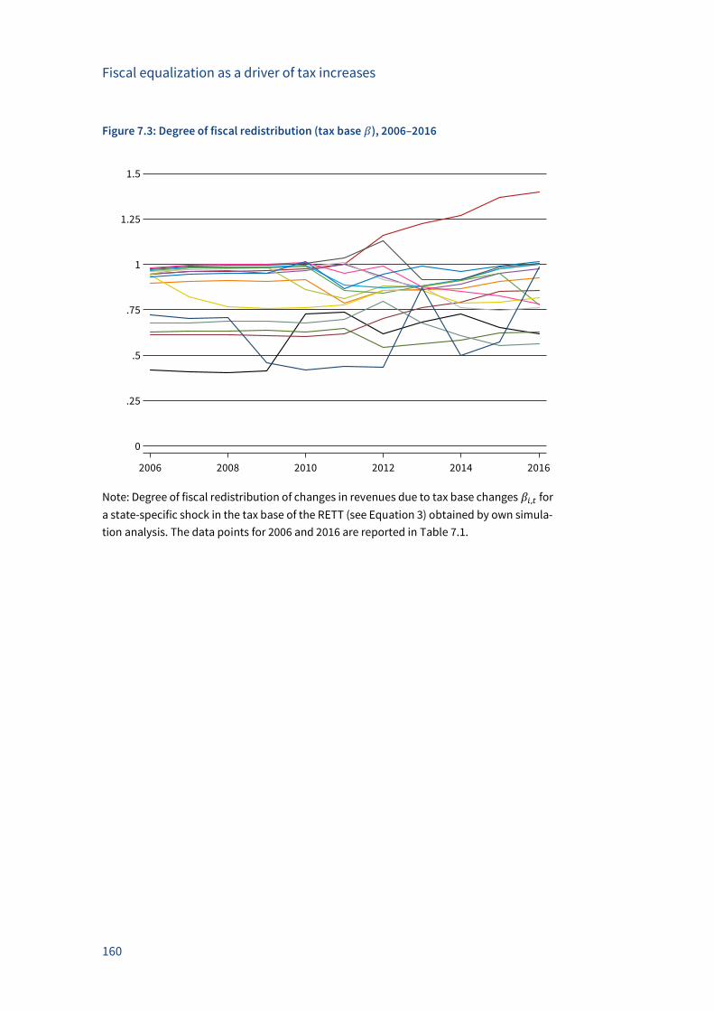
Fiscal equalization as a driver of tax increases
160
Figure 7.3: Degree of fiscal redistribution (tax base 𝛽), 2006–2016
Note: Degree of fiscal redistribution of changes in revenues due to tax base changes 𝛽𝑖,𝑡 for
a state-specific shock in the tax base of the RETT (see Equation 3) obtained by own simula-
tion analysis. The data points for 2006 and 2016 are reported in Table 7.1.
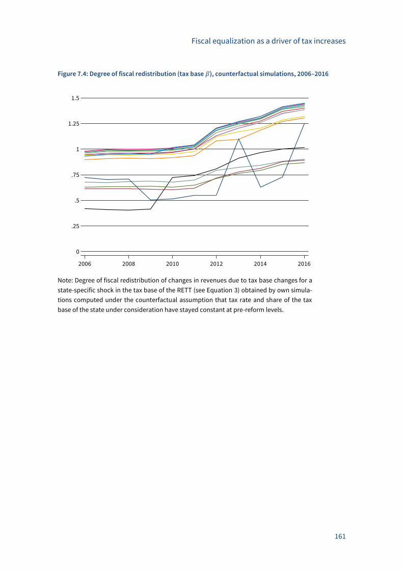
Fiscal equalization as a driver of tax increases
161
Figure 7.4: Degree of fiscal redistribution (tax base 𝛽), counterfactual simulations, 2006–2016
Note: Degree of fiscal redistribution of changes in revenues due to tax base changes for a
state-specific shock in the tax base of the RETT (see Equation 3) obtained by own simula-
tions computed under the counterfactual assumption that tax rate and share of the tax
base of the state under consideration have stayed constant at pre-reform levels.
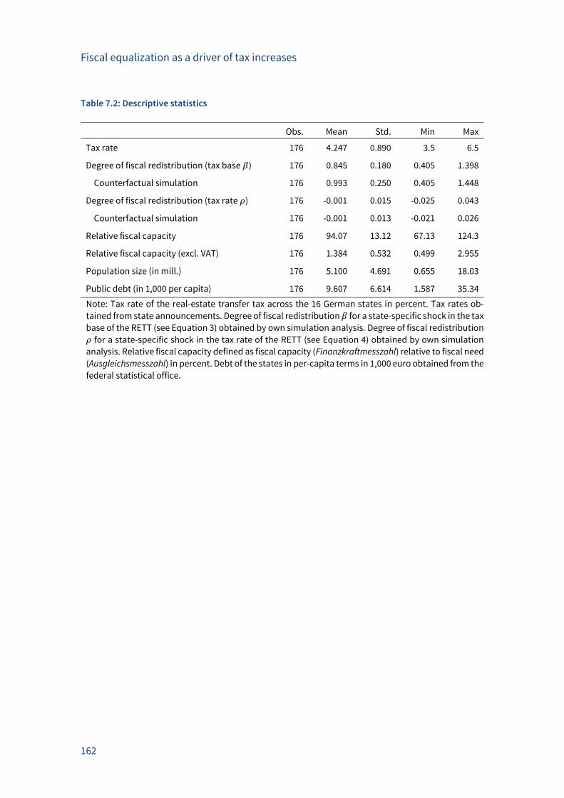
Fiscal equalization as a driver of tax increases
162
Table 7.2: Descriptive statistics
Obs. Mean Std.
Dev.
Min Max
Tax rate 176 4.247 0.890 3.5 6.5
Degree of fiscal redistribution (tax base 𝛽) 176 0.845 0.180 0.405 1.398
Counterfactual simulation 176 0.993 0.250 0.405 1.448
Degree of fiscal redistribution (tax rate 𝜌) 176 -0.001 0.015 -0.025 0.043
Counterfactual simulation 176 -0.001 0.013 -0.021 0.026
Relative fiscal capacity 176 94.07 13.12 67.13 124.3
Relative fiscal capacity (excl. VAT) 176 1.384 0.532 0.499 2.955
Population size (in mill.) 176 5.100 4.691 0.655 18.03
Public debt (in 1,000 per capita) 176 9.607 6.614 1.587 35.34
Note: Tax rate of the real-estate transfer tax across the 16 German states in percent. Tax rates ob-
tained from state announcements. Degree of fiscal redistribution 𝛽 for a state-specific shock in the tax
base of the RETT (see Equation 3) obtained by own simulation analysis. Degree of fiscal redistribution
𝜌 for a state-specific shock in the tax rate of the RETT (see Equation 4) obtained by own simulation
analysis. Relative fiscal capacity defined as fiscal capacity (Finanzkraftmesszahl) relative to fiscal need
(Ausgleichsmesszahl) in percent. Debt of the states in per-capita terms in 1,000 euro obtained from the
federal statistical office.
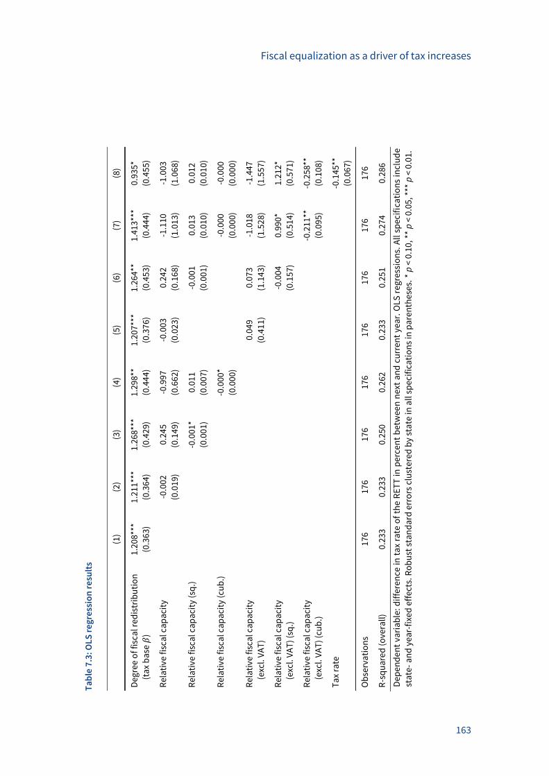
Fiscal equalization as a driver of tax increases
163
Ta
ble
7.3
: OL
S r
eg
ress
ion
re
sult
s
(1
) (2
) (3
) (4
) (5
) (6
) (7
) (8
)
Deg
ree
of f
isca
l red
istr
ibu
tio
n
(ta
x b
ase
𝛽)
1.20
8***
1.
211*
**
1.26
8***
1.
298*
* 1.
207*
**
1.26
4**
1.41
3***
0.
935*
(0.3
63)
(0
.36
4)
(0.4
29)
(0
.44
4)
(0.3
76)
(0
.45
3)
(0.4
44)
(0
.45
5)
Rel
ati
ve fi
sca
l ca
pa
city
-0.0
02
0.24
5
-0.9
97
-0.0
03
0.24
2
-1.1
10
-1.0
03
(0
.01
9)
(0.1
49)
(0
.66
2)
(0.0
23)
(0
.16
8)
(1.0
13)
(1
.06
8)
Rel
ati
ve fi
sca
l ca
pa
city
(sq
.)
-0.0
01*
0.01
1
-0.0
01
0.01
3
0.01
2
(0.0
01)
(0
.00
7)
(0
.00
1)
(0.0
10)
(0
.01
0)
Rel
ati
ve fi
sca
l ca
pa
city
(cu
b.)
-0.0
00*
-0.0
00
-0.0
00
(0
.00
0)
(0.0
00)
(0
.00
0)
Rel
ati
ve fi
sca
l ca
pa
city
(exc
l. V
AT
)
0.04
9
0.07
3
-1.0
18
-1.4
47
(0.4
11)
(1
.14
3)
(1.5
28)
(1
.55
7)
Rel
ati
ve fi
sca
l ca
pa
city
(exc
l. V
AT
) (s
q.)
-0.0
04
0.99
0*
1.21
2*
(0
.15
7)
(0.5
14)
(0
.57
1)
Rel
ati
ve fi
sca
l ca
pa
city
(exc
l. V
AT
) (c
ub
.)
-0.2
11**
-0
.258
**
(0.0
95)
(0
.10
8)
Ta
x ra
te
-0.1
45**
(0.0
67)
Ob
serv
ati
on
s 17
6
176
17
6
176
17
6
176
17
6
176
R-s
qu
are
d (
ove
rall
) 0.
233
0.
233
0.
250
0.
262
0.
233
0.
251
0.
274
0.
286
Dep
en
de
nt
vari
ab
le: d
iffe
ren
ce in
ta
x ra
te o
f th
e R
ET
T in
per
cen
t b
etw
een
nex
t a
nd
cu
rren
t ye
ar.
OLS
reg
ress
ion
s. A
ll s
pec
ific
ati
on
s in
clu
de
sta
te-
an
d y
ear-
fixe
d e
ffec
ts. R
ob
ust
sta
nd
ard
err
ors
clu
ster
ed b
y st
ate
in a
ll s
pec
ific
ati
on
s in
pa
ren
thes
es. *
p <
0.1
0, *
* p
< 0
.05,
***
p <
0.0
1.
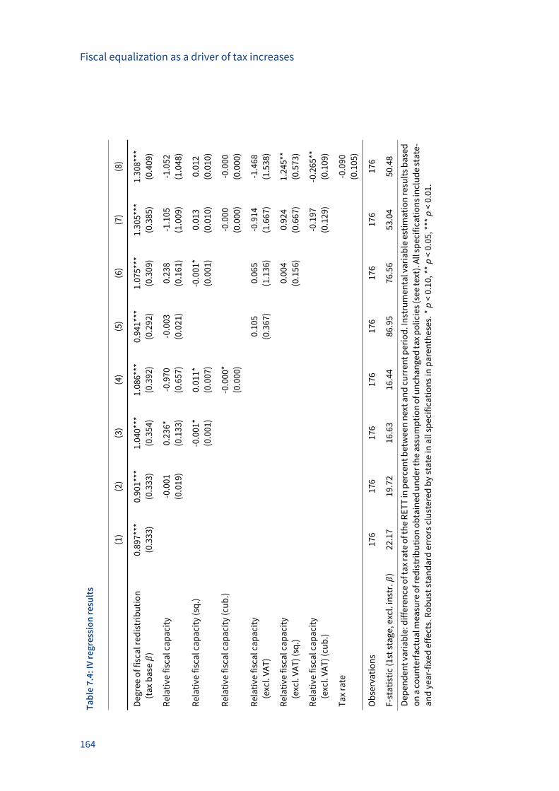
Fiscal equalization as a driver of tax increases
164
Ta
ble
7.4
: IV
re
gre
ssio
n r
esu
lts
(1
) (2
) (3
) (4
) (5
) (6
) (7
) (8
)
Deg
ree
of f
isca
l red
istr
ibu
tio
n
(ta
x b
ase
𝛽)
0.89
7***
0.
901*
**
1.04
0***
1.
086*
**
0.94
1***
1.
075*
**
1.30
5***
1.
308*
**
(0.3
33)
(0
.33
3)
(0.3
54)
(0
.39
2)
(0.2
92)
(0
.30
9)
(0.3
85)
(0
.40
9)
Rel
ati
ve fi
sca
l ca
pa
city
-0.0
01
0.23
6*
-0.9
70
-0.0
03
0.23
8
-1.1
05
-1.0
52
(0
.01
9)
(0.1
33)
(0
.65
7)
(0.0
21)
(0
.16
1)
(1.0
09)
(1
.04
8)
Rel
ati
ve fi
sca
l ca
pa
city
(sq
.)
-0.0
01*
0.01
1*
-0.0
01*
0.01
3
0.01
2
(0.0
01)
(0
.00
7)
(0
.00
1)
(0.0
10)
(0
.01
0)
Rel
ati
ve fi
sca
l ca
pa
city
(cu
b.)
-0.0
00*
-0.0
00
-0.0
00
(0
.00
0)
(0.0
00)
(0
.00
0)
Rel
ati
ve fi
sca
l ca
pa
city
(exc
l. V
AT
)
0.10
5
0.06
5
-0.9
14
-1.4
68
(0.3
67)
(1
.13
6)
(1.6
67)
(1
.53
8)
Rel
ati
ve fi
sca
l ca
pa
city
(exc
l. V
AT
) (s
q.)
0.00
4
0.92
4
1.24
5**
(0
.15
6)
(0.6
67)
(0
.57
3)
Rel
ati
ve fi
sca
l ca
pa
city
(exc
l. V
AT
) (c
ub
.)
-0.1
97
-0.2
65**
(0
.12
9)
(0.1
09)
Ta
x ra
te
-0.0
90
(0
.10
5)
Ob
serv
ati
on
s 17
6
176
17
6
176
17
6
176
17
6
176
F-st
ati
stic
(1s
t st
ag
e, e
xcl.
inst
r. 𝛽
) 22
.17
19
.72
16
.63
16
.44
86
.95
76
.56
53
.04
50
.48
Dep
en
de
nt
vari
ab
le: d
iffe
ren
ce o
f ta
x ra
te o
f th
e R
ET
T in
per
cen
t b
etw
een
nex
t a
nd
cu
rren
t p
erio
d. I
nst
rum
enta
l va
ria
ble
est
ima
tio
n r
esu
lts
ba
sed
on
a c
ou
nte
rfa
ctu
al m
easu
re o
f red
istr
ibu
tio
n o
bta
ined
un
der
the
ass
um
pti
on
of u
nch
an
ged
ta
x p
olic
ies
(se
e te
xt).
All
sp
ecif
ica
tio
ns
incl
ud
e st
ate
-
an
d y
ear-
fixe
d e
ffec
ts. R
ob
ust
sta
nd
ard
err
ors
clu
ster
ed b
y st
ate
in a
ll s
pec
ific
ati
on
s in
pa
ren
thes
es. *
p <
0.1
0, *
* p
< 0
.05,
***
p <
0.0
1.
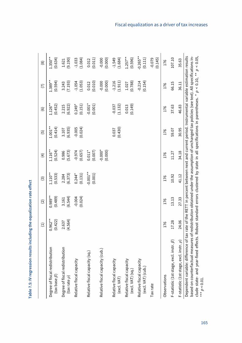
Fiscal equalization as a driver of tax increases
165
Ta
ble
7.5
: IV
re
gre
ssio
n r
esu
lts
incl
ud
ing
th
e e
qu
ali
zati
on
ra
te e
ffe
ct
(1
) (2
) (3
) (4
) (5
) (6
) (7
) (8
)
Deg
ree
of f
isca
l red
istr
ibu
tio
n
(ta
x b
ase
𝛽)
0.96
2**
0.98
9**
1.11
0**
1.11
6**
1.00
1**
1.12
6**
1.38
9**
1.35
0**
(0.4
22)
(0
.48
9)
(0.5
33)
(0
.52
4)
(0.4
14)
(0
.45
2)
(0.5
94)
(0
.63
4)
Deg
ree
of f
isca
l red
istr
ibu
tio
n
(ta
x ra
te 𝜌
)
2.63
7
3.16
1
2.28
4
0.98
6
3.10
7
2.21
5
3.24
3
1.62
1
(4.5
64)
(6
.54
4)
(6.3
73)
(5
.67
3)
(6.9
35)
(6
.92
2)
(7.1
93)
(9
.19
0)
Rel
ati
ve fi
sca
l ca
pa
city
-0.0
04
0.24
4*
-0.9
74
-0.0
05
0.24
9*
-1.0
54
-1.0
33
(0
.02
4)
(0.1
31)
(0
.65
7)
(0.0
24)
(0
.15
1)
(1.0
53)
(1
.08
4)
Rel
ati
ve fi
sca
l ca
pa
city
(sq
.)
-0.0
01**
0.
011*
-0.0
01*
0.01
2
0.01
2
(0.0
01)
(0
.00
7)
(0
.00
1)
(0.0
10)
(0
.01
1)
Rel
ati
ve fi
sca
l ca
pa
city
(cu
b.)
-0.0
00*
-0.0
00
-0.0
00
(0
.00
0)
(0.0
00)
(0
.00
0)
Rel
ati
ve fi
sca
l ca
pa
city
(exc
l. V
AT
)
0.03
7
-0.0
37
-1.2
16
-1.5
49
(0.4
30)
(1
.13
2)
(1.9
11)
(1
.68
4)
Rel
ati
ve fi
sca
l ca
pa
city
(exc
l. V
AT
) (s
q.)
0.01
3
1.02
7
1.25
7**
(0
.14
9)
(0.7
88)
(0
.59
6)
Rel
ati
ve fi
sca
l ca
pa
city
(exc
l. V
AT
) (c
ub
.)
-0.2
14
-0.2
65**
(0
.15
4)
(0.1
11)
Ta
x ra
te
-0.0
79
(0
.14
5)
Ob
serv
ati
on
s 17
6
176
17
6
176
17
6
176
17
6
176
F-st
ati
stic
(1s
t st
ag
e, e
xcl.
inst
r. 𝛽
) 17
.28
13
.13
10
.92
11
.27
59
.07
37
.63
66
.15
10
7.1
0
F-st
ati
stic
(1s
t st
ag
e, e
xcl.
inst
r. 𝜌
) 24
.06
27
.33
41
.12
34
.18
30
.95
46
.83
36
.11
35
.63
Dep
en
de
nt
vari
ab
le:
dif
fere
nce
of
tax
rate
of
the
RE
TT
in
per
cen
t b
etw
een
ne
xt a
nd
cu
rren
t p
erio
d.
Inst
rum
enta
l va
ria
ble
est
ima
tio
n r
esu
lts
ba
sed
on
co
un
terf
act
ua
l me
asu
res
of
red
istr
ibu
tio
n o
bta
ined
un
der
th
e a
ssu
mp
tio
n o
f u
nch
an
ged
ta
x p
oli
cies
(se
e te
xt).
All
sp
ecif
ica
tio
ns
in-
clu
de
sta
te-
an
d y
ear-
fixe
d e
ffec
ts.
Ro
bu
st s
tan
da
rd e
rro
rs c
lust
ered
by
sta
te i
n a
ll s
pec
ific
ati
on
s in
pa
ren
thes
es.
* p
< 0
.10,
**
p <
0.0
5,
***
p <
0.0
1.
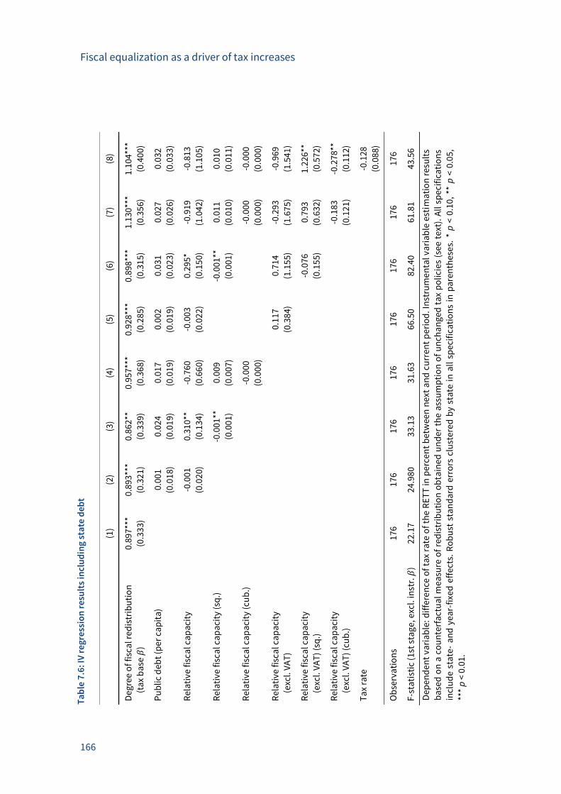
Fiscal equalization as a driver of tax increases
166
Ta
ble
7.6
: IV
re
gre
ssio
n r
esu
lts
incl
ud
ing
sta
te d
eb
t
(1
) (2
) (3
) (4
) (5
) (6
) (7
) (8
)
Deg
ree
of f
isca
l red
istr
ibu
tio
n
(ta
x b
ase
𝛽)
0.89
7***
0.
893*
**
0.86
2**
0.95
7***
0.
928*
**
0.89
8***
1.
130*
**
1.10
4***
(0.3
33)
(0
.32
1)
(0.3
39)
(0
.36
8)
(0.2
85)
(0
.31
5)
(0.3
56)
(0
.40
0)
Pu
blic
deb
t (p
er c
ap
ita
)
0.00
1
0.02
4
0.01
7
0.00
2
0.03
1
0.02
7
0.03
2
(0
.01
8)
(0.0
19)
(0
.01
9)
(0.0
19)
(0
.02
3)
(0.0
26)
(0
.03
3)
Rel
ati
ve fi
sca
l ca
pa
city
-0.0
01
0.31
0**
-0.7
60
-0.0
03
0.29
5*
-0.9
19
-0.8
13
(0
.02
0)
(0.1
34)
(0
.66
0)
(0.0
22)
(0
.15
0)
(1.0
42)
(1
.10
5)
Rel
ati
ve fi
sca
l ca
pa
city
(sq
.)
-0.0
01**
0.
009
-0.0
01**
0.
011
0.
010
(0
.00
1)
(0.0
07)
(0.0
01)
(0
.01
0)
(0.0
11)
Rel
ati
ve fi
sca
l ca
pa
city
(cu
b.)
-0.0
00
-0.0
00
-0.0
00
(0
.00
0)
(0.0
00)
(0
.00
0)
Rel
ati
ve fi
sca
l ca
pa
city
(exc
l. V
AT
)
0.11
7
0.71
4
-0.2
93
-0.9
69
(0.3
84)
(1
.15
5)
(1.6
75)
(1
.54
1)
Rel
ati
ve fi
sca
l ca
pa
city
(exc
l. V
AT
) (s
q.)
-0.0
76
0.79
3
1.22
6**
(0
.15
5)
(0.6
32)
(0
.57
2)
Rel
ati
ve fi
sca
l ca
pa
city
(exc
l. V
AT
) (c
ub
.)
-0.1
83
-0.2
78**
(0
.12
1)
(0.1
12)
Ta
x ra
te
-0.1
28
(0
.08
8)
Ob
serv
ati
on
s 17
6
176
17
6
176
17
6
176
17
6
176
F-st
ati
stic
(1s
t st
ag
e, e
xcl.
inst
r. 𝛽
) 22
.17
24
.98
0
33.1
3
31.6
3
66.5
0
82.4
0
61.8
1
43.5
6
Dep
en
de
nt
vari
ab
le: d
iffe
ren
ce o
f ta
x ra
te o
f th
e R
ET
T in
per
cen
t b
etw
een
ne
xt a
nd
cu
rren
t p
erio
d. I
nst
rum
en
tal v
ari
ab
le e
stim
ati
on
res
ult
s
ba
sed
on
a c
ou
nte
rfa
ctu
al
mea
sure
of
red
istr
ibu
tio
n o
bta
ine
d u
nd
er t
he
ass
um
pti
on
of
un
cha
ng
ed t
ax
po
lici
es (
see
tex
t).
All
sp
ecif
ica
tio
ns
incl
ud
e st
ate
- a
nd
yea
r-fi
xed
eff
ects
. R
ob
ust
sta
nd
ard
err
ors
clu
ster
ed
by
sta
te i
n a
ll s
pec
ific
ati
on
s in
pa
ren
thes
es.
* p
< 0
.10,
**
p <
0.0
5,
***
p <
0.0
1.
Conclusion
167
8 Conclusion
Conclusion
I have elaborated on selected incentives in fiscal federalism by using the example of the fed-
eral system in Germany. Many countries have decentralized governments aiming to improve
the performance of the public sector. The allocation of tasks and public services to different
levels requires however a well-designed institutional structure. The decentralization of public
services and tasks is thus combined with an allocation of spending and financing responsibil-
ities to ensure the autonomy of subnational governments. Federations also implement equal-
ization schemes or provide intergovernmental grants to subnational governments to reduce
disparities between subnational regions. The combination of autonomy and equalization may
however provide incentives to reduce efforts in generating own revenues. The behavior of pol-
iticians may also influence economic policy-making. Public choice theories suggest that poli-
ticians are self-interested and maximize own welfare rather than social welfare.
My studies provide mixed evidence for political and fiscal incentives within Germany’s feder-
alism. Chapters 2 and 3 examined election cycles, based on the political business cycle theo-
ries. The political business cycle theories describe that politicians are likely to increase their
reelection chances by pursuing expansionary policies before elections. In Chapter 2, I exam-
ined whether election cycles occur in fees of German municipalities. Fees are interesting to
investigate as they are levied according to the benefit principle. Fees have to be equivalent to
the (expected) costs of the public service they are levied on. This should constrain govern-
ments. My results show however that municipalities have a leeway to decide on fees and use
this leeway to improve election prospects. Fees increase less in election years and increase
more directly after elections than in the middle of the legislative period. The results of Chapter
3 show however that governments do not always use their discretionary power. In joint work
with my co-authors, I analyzed salary increases of German state MPs, for which the states have
the decision-making authority. The results do not show that electoral motives influence in-
creases in MP salaries. Politicians can, by contrast, increase their salaries at any point in time.
In Chapters 4 and 5, I investigated how government ideology influences economic policy-mak-
ing. Partisan theories describe that left-wing and right-wing governments pursue different
policies in line with the preferences of their constituencies. The evidence of my studies is how-
ever mixed. In Chapter 4, which is based on joint work with my co-authors, I analyzed whether
government ideology influences income inequality in the public sector of the German states.
We used data on salaries of civil servants and calculated several income inequality measures.
The results do not show that left-wing governments were more active in decreasing income
inequality in the public sector than center or right-wing governments. The results of Chapter
5, by contrast, show that left-wing and right-wing governments may well differ in their poli-
cies. In joint work with my co-author, I analyzed whether government ideology predicts tax
policies of the German states. A reform of the fiscal constitution in 2006 allowed the states to
Conclusion
168
set the tax rates of the real-estate transfer tax. By investigating the tax rate increases of the
German states from 2007 onwards, our results show that left-wing governments were more
active in increasing the tax rates than right-wing governments.
Chapters 6 and 7 investigate fiscal incentives within the federal system in Germany. In joint
work with my co-author, I analyzed whether the institutional setting in Germany also provides
incentives for states’ tax policies. The German fiscal equalization scheme redistributes reve-
nues among the federal and state level and between states equalizing funds for the states.
The devolution of tax setting powers to the states in 2006 provides an interesting set-up to
investigate the combination of tax autonomy and fiscal equalization. The descriptive results
in Chapter 6 and the empirical analysis in Chapter 7 show that equalization substantially in-
fluences tax policies of the states. The redistribution of revenues within the equalization
scheme provides incentives for the states to raise rather than to lower their tax rates.
The results of my thesis show that political and fiscal incentives may well influence economic
policy-making. Electoral motives and government ideology can explain parts of individual
economic policies. Citizens should thus be aware of the given leeway of politicians in several
policy fields. The mixed evidence on political incentives however also shows that politicians
are not always prone to manipulate economic policy-making. Important to note is also that
the interpretation of results depends crucially on how the empirical analyses were conducted.
I only rely on correlations when examining partisan effects. Government ideology variables
are likely to be endogenous. One concern is reverse causality. Omitted variable bias concerns
play however also a role. It was not possible to identify causal effects when analyzing partisan
effects because of too small samples. Possible policy implications from analyses of partisan
effects have to take this shortcoming into account. Future research thus needs to find a way
to overcome the endogeneity problem of government ideology variables to identify causal
effects of partisanship – also when samples are small.
I also show that the institutional set-up in federal systems may provide incentives for govern-
ments. Chapters 6 and 7 show that the combination of tax autonomy and fiscal equalization
distort tax policies in the German states. This result is relevant for policymakers and also for
the public debate. A well-designed institutional setting has to rule out distortive incentives. In
Chapter 6, we propose a solution to overcome the distortive incentive effect of fiscal equali-
zation on tax policy. This recommendation could serve as a starting point for policymakers to
reform fiscal equalization in Germany in the near future.
Many countries implemented federal systems aiming to improve the performance of the pub-
lic sector. Every federal system needs however also a well-designed institutional structure to
limit distortive incentives. Decentralized governments can improve welfare. Important is that
they improve social welfare and not politicians’ welfare. As the philosopher and political the-
orist Edmund Burke stated:

Conclusion
169
“Government is a contrivance of human wisdom to provide for human wants.
Men have a right that these wants should be provided for by this wisdom.”

Conclusion
170
Curriculum Vitae
171
Curriculum Vitae
Curriculum Vitae
Manuela Maria Krause
born on June 19, 1989 in Wickede (Ruhr), Germany
since 02/2015 Ph.D. Candidate, Munich Graduate School of Economics,
Ludwig-Maximilians-Universität, Munich
Junior Economist and Doctoral Student,
Ifo Institute – Leibniz Institute for Economic Research
at the University of Munich
10/2011 – 09/2014 Master of Science in Economics,
University Bielefeld
10/2008 – 09/2011 Bachelor of Science in Economics,
University Bielefeld
06/2008 Abitur (High School Diploma),
Walburgisgymnasium Menden (Sauerland)

172