enclosure methods - kit
TRANSCRIPT
Enclosure Methods
G. AlefeldInstitut für Angewandte Mathematik
Universität KarlsruheFederal Republic of Germany
Abstract: We present an overview on existing methods for inc1uding the range of
functions by interval arithmetic tools.
1. Introduction
In this paper we do not try to give a precise definition oE what we mean by an
enclosure method. Instead we first recall that the four basic interval operations
allow to inc1ude the range of values oE rational Eunctions. Using more appropriate
tools also the range oE more general functions can be included. Since all enclosure
methods for the solution of equations which are based on interval arithrnetic tools
are finally enc10sure methods for the range of some function we concentrate our-
selves on rnethods fo~ the inc1usion oE the range oE functions. We limit our dis-
cussion to the case oEfunctions oE one real variable. Most oE the material in the
present paper is weIl known. See [1], Chapter 3 and the books [9], [10] by
Ratschek and Rokne, for example. However, there are also some new results. See
Theorem 2, for example.
Computer Arithmetic and Self-ValidatingNumerical Methods
55 Copyright @ 1990 by Academic Press, Inc.All rights of reproduction in any form reselVed.
ISBN O-12-708245-X
56 G. Alefeld
2. Notation
Tbe notation in tbis paper is essentially tbe same as in [1]. We repeat tbe most
irnportant ones in order tbat tbe non-specialist can also read tbis paper. Real
intervals [a1;~]' [b1;b2]'''' are denoted by [a], [b],... . Tbe four arithrnetic
operations for intervals are defined by
[a]*[b] = {a*bla E [a], b E [b]}, * E {+,-,x,j} .
Tbe result is an interval wbose bounds can be computed from tbe bounds of [a]
and [b] . Similarly, vectors witb intervals as components, so-called interval
vectors, are denoted by [a] = ([a].) , [b] = ([b].) ,... . Analogously, [A] = ([a]..)1 1 IJ
denotes an interval matrix. m[a] is tbe center of [a], d[a] = a2-a1 is tbe
diameter of [a], q([a],[b]) = max{la1-bl' , la2-b2'} denotes tbe distance of
[a] and [b] and q([a],O) = '[a] I is called tbe absolute value of [a]. Tbese
concepts are defined for interval vectors and interval matrices via tbe components.
For additional details we refer to [1].
3. Interval aritbmetic evaluation
The four basic operations for intervals are inclusion monotone:
If [a].c [c] , [b] .c [d] tben [a]*[b] .c [c]*[d] , * E {+,-,x,j} .
From tbis it follows tbat for rational functions (and more generally for all
functions f whicb bave an interval aritbmetic evaluation (see [1], Cbapter 3» tbe
range R(f;[x]) of f over tbe interval [x] is contained in tbe interval aritbmetic
evaluation f([x]):
~,.
Enclosure Metluxis 57
(1) R(f;[x]) ~ f([x]) .
Example 1. Let
fex) = l~x ' x -f 1
and [x] = [2 ; 3] . Then
3R(f;[xJ) = [-2 ; - 2] ,
f([x]) = ~ = AA = [-3 ; -1] ,
and therefore R(f;[x]) c f([x]) holds.
For x -f 0 we can rewrite fex) as
x 1fex) = I-x = r-: ' x -f 0 .- - 1x
For the interval arithmetic evaluation of this function over [2;3] we get
1 3f ([x]) = 1 = [-2 ; - 2] = R(f;[x]).
[2;31 - 1
"
0
The preceding example shows that the overestimation of R(f;[x]) by f([x]) is
strongly dependent on the arithmetic expression which is used for the interval
arithmetic evaluation of the given function.
58 G. Alefeld
Moore [6] has shown that under reasonable assumptions the following inequality
holds für the distance between R(f;[x)) and f([x]):
(2) q(R(f;[x)) , f([x))) ~ I d[x] , [x] ~ [xf , I ~ 0 .
This means that the overestimation of R(f;[x]) by f([x)) goes linearly to zero
with d[x]. We illustrate this using the following example.
Example 2. Let
2fex) = x - x , x E [xf = [0;1] .
Set111
[x] = [2 - r ; 2 + r] , 0 ~ r ~ 2 .
A simple discussion gives
121R(f;[x)) = [4 - r ; 4] .
Für f([x)) we get
1 1 1 1 1 1f([x]) = [2 - r ; 2 + r] - [2 - r ; 2 + r][2 - r ; 2 + r]
1 2 1 2= [4 - 2r - r ; 4 + 2r - r ] .
From this we get
1 2121 21q(R(f;[x)) , f([x])) = max {14 - 2r - r - 4 + r I , 14 + 2r - r - 41}
Enclosure Methods 59
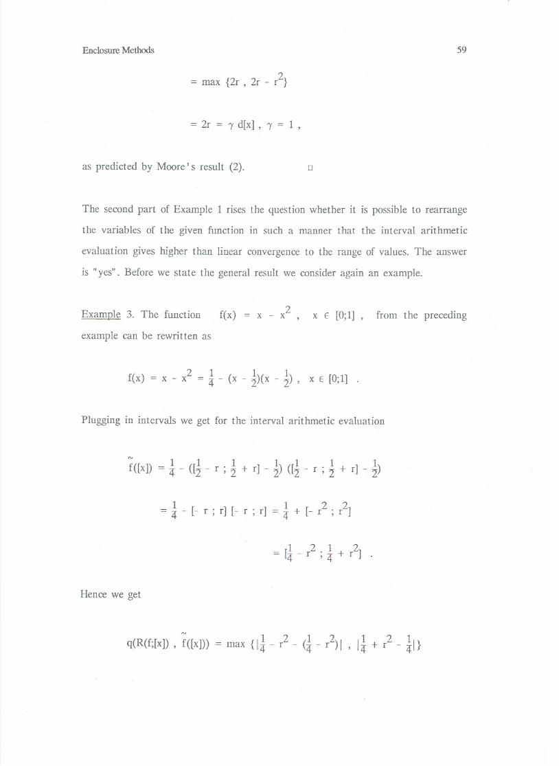
2= max {2r , 2r - r }
= 2r = 1 d[x] , 1 = 1 ,
as predicted by Moore I s result (2). 0
The second part of Example 1 rises the question whether it is possible to rearrange
the variables of the given function in such a mann er tbat the interval arithmetic
evaluation gives higher than linear convergence to the range of values. The answer
is "yes". Before we state tbe general result we consider again an example.
Example 3. The function2
fex) = x - x x E [0;1] , from the preceding
example can be rewritten as
2 1 1 1 .fex) = x - x = 4 - (x - 2)(x - 2)' x E [0,1] .
Plugging in intervals we get for the interval aritbmetic evaluation
NIl 1 11 1 1f([x)) = 4 - ([2 - r ; 2 + r] - 2) ([2 - r ; 2 + r] - 2)
1 1 2 2= 4 - [- r ; r] [- r ; r] = 4 + [- r ; r ]
1 2 1 2=[4-r ;4+r].
Hence we get
N 1212121q(R(f;[x]) , f([x]» = max {14 - r - (4 - r )1 , 14 + r - 41}

60 G. Alefeld
2 1 2= r = 4(d[x])
which means that the distance goes quadratically to zero with d[x] .
The general result is as follows:
(The centered form). Let the (rational) function f:IR...,1R beTheorem 1.
represented in the form
(3) f(x) = f(z) + (x-z) . h(x)
for some z E [x] . If we define
(4) f([x]) := f(z) + ([x] - z) h([x])
then (under weak conditions on the interval arithmetic evaluation h([x]) , see
Theorem 2) it holds that
a) R(f;[x)) .c f([x])
and
(5) b)2
q(R(f;[x)) , f([x])) ~ I (d[x]) . 0
Inequality (5) is called "Quadratic approximation property" of the centered form.
(3) was introduced by Moore in [6], where he conjectured that (5) holds. (5) was
first proved by E. Hansen [5].
Enclosure Methods 61
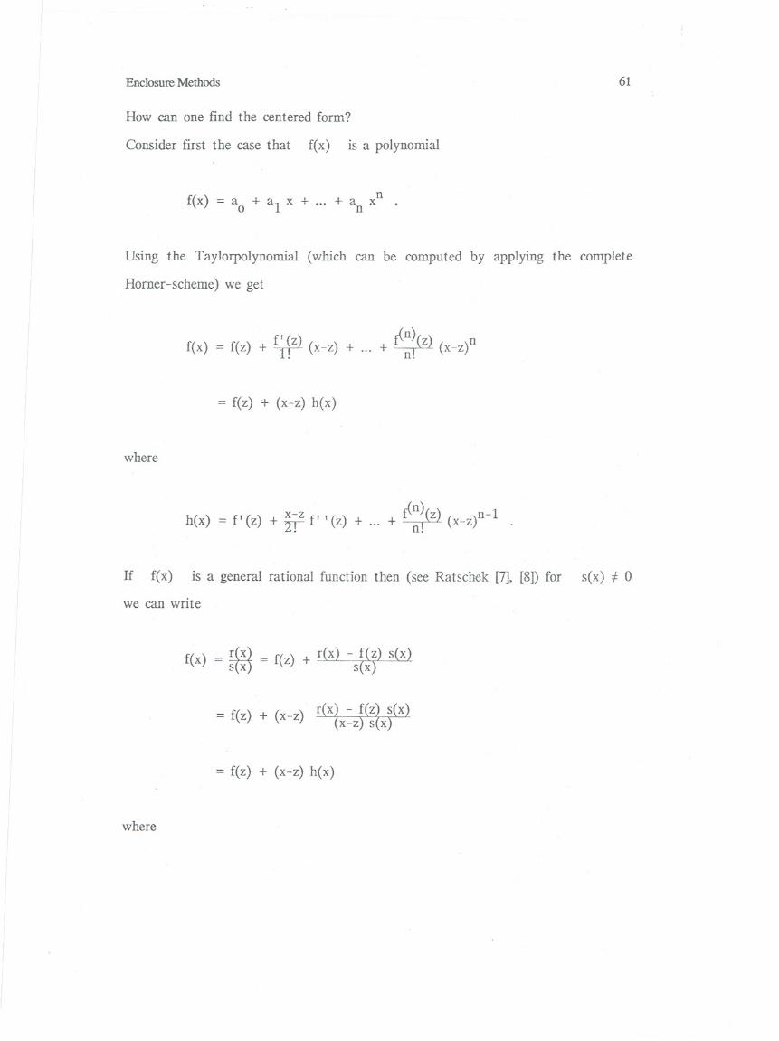
How can one find the centered form?
Consider first the case that fex) is a polynornial
fex) = a + a l x + ... + a xn0 n
Using the Taylorpolynornial (which can be computed by applying the complete
Horner-scheme) we get
f' (z) t<n~(z) nfex) = fez) + 1! (x-z) + ... + n. (x-z)
= fez) + (x-z) hex)
where
hex) = f' (z) + ~!z fl '(z) + ... + t<:~(Z) (x_z)n-l .
If fex) is a general rational function then (see Ratschek [7], [8]) for sex) :{ 0
we can write
fex) = rex} = fez) + rex) - fez) sex)sw sex)
= fez) + (x-z) r(x~ - f(z~ sex)x-z) s x)
= fez) + (x-z) hex)
where

-
62 G. Alefeld
hex) = r(x~ - f(z~ sex)x-z) s x) .
Since r(z) - fez) s(z) = 0 and s(z) f- 0 the term x-z appears both in
the nominator and in the denominator of hex) and therefore can be cancelled
out.
Example 4. Let
2
*fx x-x
fex) = = ~, x f- 3 .s x X-.J
For 1 1z = 2 wehave fez) = - 10 and therefore
f(x) ~ - fu + (x - 1) r(x) - (- fu) s(x)2 1(x - 2) sex)
1_ (1 1 1
= - 1 + (X 1)4 x - 2) (x - 2) - (- ~) «x - 1) - 5)
ID -2 1 UY 2 2(x - 2) «x - i) - ~)
- 1 1 1- - ID + (x - 1)
10 - (x - )2 5 2
- 2 + (x - i)
= -k + (x - i) hex)
where
1 1
hex) = ID - (x - 2)5- 2 + (x - i) .
0

Enc10sure Methods 63
The quest ion whether there exists a representation of f such that for the
interval arithmetic evaluation of this representation it holds that
q(R(f;[x]), f([x]) ~ J (d[x])m
where m ~ 3 is an open question. However, in special cases this can be
achieved.
Theorem 2. (Generalized centered forms). Let the (rational) function f:IR--71R
be represented in the form
(6) fex) = <p + fex) . hex) ,0 x E [x] ,
where <p E IR . Assume that there exist intervals0 f([x]) and h([x]) such
that
(7) fex) E f([x]), x E ([x]) ,
(8) hex) E h([x]), x E [x] ,
(9) If([x])I ~ T(d[x])n,
(10) d(h([x]) ~ (j d[x] .
If we define

64 G. Alefeld
(11) f([x]) := <Po + R(e;[x]) . h([x])
then
(12) R(f;[x]) ~ f([x]) ,
(13) q(R(f;[x]) , f([x])) ~ ~(d[x])n+1 . 0
A proof of Theorem 2 has been performed in [1J.
Example 5. a) Assume that
(14) fex) = (x-c)n, C E [xJ .
Then
If([xJ)I = I ([xJ - c)n I ~ (d[x])n
and therefore (9) holds.
Für n = 1 in (14) we have the c1assical centered form (see Theorem 1). For
n > 1 in (14) the result of Theorem 2 was al ready proved in [2].
b) Assume that
(15) fex) = (x-x l ) . ... . (x-x), x. E [xJ, i = l(l)n .n 1
Enclosure Methods 65
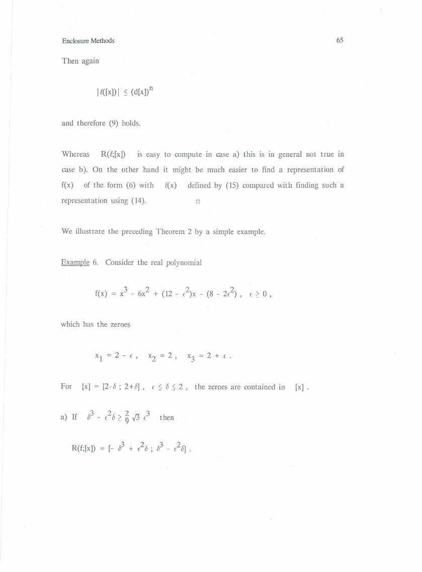
Then again
If([x]) I ~ (d[x])n
and therefore (9) holds.
Whereas R(f;[x]) is easy to compute in case a) this is in general not true in
case b). On the other hand it might be much easier to find a representation of
f(x) of the form (6) with f(x) defined by (15) compared with finding such a
representation using (14). 0
We illustrate the preceding Theorem 2 by a simple example.
Example 6. Consider the real polynomial
3 2 2 2f(x) = x - 6x + (12 - ( )x- (8 - 2( ), (~O,
which has the zeroes
Xl = 2 - ( , x2 = 2, x3 = 2 + ( .
For [X] = [2-5 ; 2+b), (~5 ~ 2, the zeroes are contained in [X]-
a) If /53 - (2 /5 ~ ~ IJ (3then
R(f;[x]) = [- /53 + (25; 53 - (2b) .

66
b) If b3 - f.2b < ~ .ß f.3then
2 3R(f;[x]) = g .ß f. [- 1 ; 1] .
We consider three different cases for the inclusion of
evaluation of interval expressions.
A) f([x]) = f([2-b ; 2+b])
3 2 3 2=[- {j + bt - 48b ; /j - f. (j + 48b]
from which it follows that
q(R(f;[x]) , f([x]) ~ I d[x] .
This agrees with Moore' s result (2).
B) fex) can be written as
fex) = <p + fex) . hex)0
where 2 2<Po = 0, fex) = x - 2, hex) = x - 4x + 4 - f. .
From this we get
f([x]) := cp + R(f;[x]) . h([x])0
R(f;[x ])
G. Alefeld
by the

Enc10sure Methods
= [- 0 ; 0] ([2-0 ; 2+0][2-0 ; 2+0] - 4[2-0 ; 2+0] + 4 - (2)
= [- 03 + &2 - 802 ; 03 - &2 + 802]
and therefore
2q(R(f;[x]) , f([x))) ~ I (d[x])
which agrees with the statement (5) of Theorem 1.
C) If we write fex) as
fex) = <P + fex) . hex)0
where
<Po = 0, fex) = (x-2) (x - (2+t)) , hex) = x - (2-t)
then
(16) f([x]) = <p + R(f;[x)) . h([x])0
2
= [min {- f- (0 + t), - (0 - t)(02 + tO)} ;
2 2max { ~ (0 - t), (8 + tO)(o + t)}]
and therefore
67
68 G. Alefeld
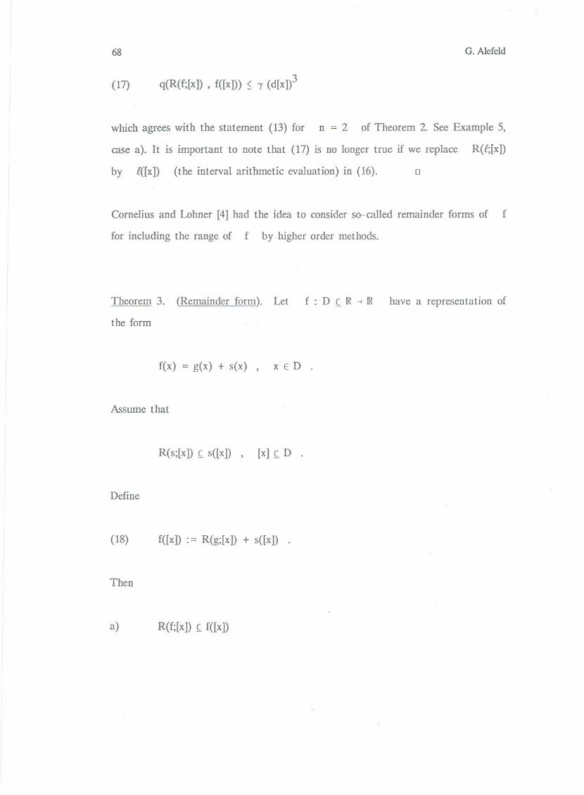
(17) q(R(f;[x]) , f([x]) ~ I (d[x])3
which agrees with the statement (13) für n=2 of Theorem 2. See Example 5,
case a). It is important to note that (17) is no longer true if we replace . R(f;[x])
by f([x]) (the interval arithmetic evaluation) in (16). 0
Cornelius and Lohner [4] had the idea to consider so-called remainder forms of f
for including the range of f by higher order methods.
Theorem 3. (Remainder form). Let
the form
f:DhlR--!1R have a representation of
f(x) = g(x) + s(x) , x E D .
Assume that
R(s;[x]) h s([x]) , [x] h D .
Define
(18) f([x]) := R(g;[x]) + s([x]) .
Then
a) R(f;[x]) h f([x])

Enclosure Methods 69
b) q(R(f;[x]) , f([x]) ~ d(s([x]) ~ 2\ s([x])I 0
0
How can one find a remainder form of f ?
Suppose that f has derivatives of sufficiently high order. Let pa(x)be the
unique polynornial of degree a ~ 0 solving the Herrnite interpolation problem:
(19) p (j)(x.) = Ij)(x.) 0all j = O(l)m. - 1, m. EIN,1 1
i = O(l)n, n ~ 0 ,
where xO' Xl' 0.. , xn E [x] are pairwise distinct and
n
a + 1 = L mi1=0
Then it is weIl known that
(20)la+1) ») n m.
fex) = p (x) + (+ H~x n (x-x.) 1a a o' 11=0
= g(x) + sex) , X E [x]
where we have set g(x) = p (x) and sex) is the remainder term. Assumea
now that the derivative I a+ 1) has an interval arithmetic evaluation over [x].
Then, since ~(x) E [x] , we can set
s([x]) = la + 1)~~( rd-l
n m.n ([x]-x.) 1. 1
1=0
70 G. Alefeld
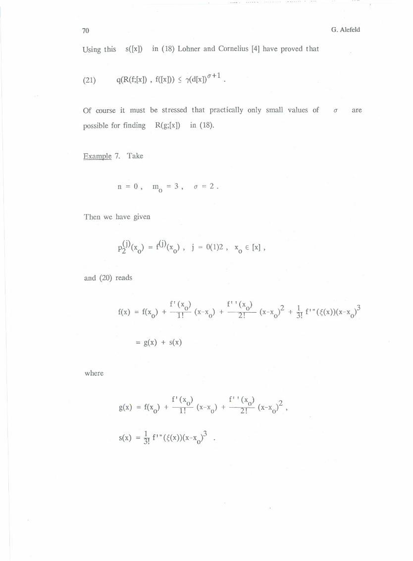
Using this s([x]) in (18) Lohner and Cornelius [4] have proved that
(21) q(R(f;[x]) , f([x]) ~ i(d[x])o-+1 .
Of course it IDust be stressed that practically only small values of 0- are
possible for finding R(g;[x]) in (18).
Exarnple 7. Take
n = 0, rn =30 '
0- = 2 .
Then we have given
p~j)(xo) = Ij)(xo)' j = 0(1)2, Xo E [x] ,
and (20) reads
f' (x ) f' '(x)0(
0 2 1 3fex) = fex ) + I' x-x) + 2' (x-x) + "IT flll(~(X»(x-x o)0 - 0 . o.J:
= g(x) + sex)
where
f' (x ) f' I (x )0)
0 2g(x) = f(xo) + I' (x-x + 2' (x-x),. 0 . 0
sex) = ~ f'" (~(x»(x-xo)3 .

Enclosure Methods 71
R(g;[x]) is easy to compute in this case since
For
g(x) is a quadratic polynornial.
f([x]) := R(g;[x]) + fu f' "([x])([x]-xo)3
we have by (21)
3q(R(f;[x]) , f([x])) ~ ,(d[x]) . 0
4. Outlook
The discussion in the preceding chapter shows that although it is easy to include
the range of functions using interval arithmetic tools it is in general not obvious
how to find very good inclusions with a reasonable amount of work. Therefore this
problem needs very careful furt her investigations.
We have not considered functions of several variables. From a practical point of
view including the range of such a function is even of much greater importance.
See [10], for example, where optimization algorithms, based on interval arithmetic
tools, are discussed. In principle all results of the present paper hold for the
multidimensional case. However, getting good inclusions is in general much more
laborious than for the one dimensional case.
References
[1] Alefeld, G.: On the approximation of the range of values by interval
expressions. Submitted for publication.
72 G. Alefeld
(2] Alefeld, G., Lohner, R: On higher order centered fonns. Computing 35,
177-184 (1985).
[3] Alefeld, G., Herzberger, J.: Introduction to Interval Computations.
New York: Academic Press 1983.
[4] Corne1ius,H., Lohner, R: Computing the range of values with accuracy higher
than second order. Computing 33, 331-347 (1984).
[5] Hansen, E.R: The centered form. In Topics in Interval Analysis,
ed. E. Hansen. Oxford 1969, pp. 102-105.
[6] Moore, RE.: Interval Analysis. Prentice Hall, Englewood Cliffs, N. J., 1966.
[7] Ratschek, H.: Zentrische Formen. Z. Angew. Math. Mech. 58 (1978),
T 434- T 436.
[8] Ratschek, H.: Centered forms. SIAM Journal on Numerical Analysis, 17,
656-662, 1980.
[9] Ratschek, H., Rokne, J.: Computer Methods for the Range of Functions.
Ellis Horwood, Chichester (1984).
[10] Ratschek, H., Rokne, J.: New Computer Methods for Global Optimization.
Ellis Horwood, Chichester (1988).