Engineering Design with Digital Thread

Victor Singh* and Karen E. Willcox�

Massachusetts Institute of Technology, Cambridge, MA, 02139

Digital Thread is a data-driven architecture that links together information generatedfrom across the product lifecycle. Though Digital Thread is gaining traction as a digitalcommunication framework to streamline design, manufacturing, and operational processesin order to more efficiently design, build and maintain engineering products, a principledmathematical formulation describing the manner in which Digital Thread can be used forcritical design decisions remains absent. The contribution of this paper is to present sucha formulation from the context of a data-driven design and decision problem under uncer-tainty. This formulation accounts for the fact that the design process is highly iterative andnot all information is available at once. Output design decisions are made not only on whatdata to collect but also on the costs and benefits involved in experimentation and sensorinstrumentation to collect that data. The mathematical formulation is illustrated throughan example design of a structural fiber-steered composite component. In this example,the methodology highlights how different sequencing of small-scale experimentation withmanufacturing and deployment lead to different designs and different associated costs.

Nomenclature

Aklt Policy parametrization matrix coeffi-cients for ply angle at stage t

Dt Digital Thread at stage tFmt Failure index for failure mode m at

stage tItotalt Total complexity at stage tIt Information space over available re-

sources at stage tIfibt Fiber complexity at stage tIthickt Thickness complexity at stage tK Number of spatial basis functions used

per stageL Number of Digital Thread feature ba-

sis functions used per stageM Number of structural failure modesPt Probability space for uncertain input

variables at stage tTt Space of all tools, methods, and pro-

cesses at stage tVt Value function at stage tVt Space of design and manufacturing pa-

rameters for all products at stage tZklt Policy parametrization matrix coeffi-

cients for thickness at stage tcfibt , c

thickt Weighting coefficients for fiber and

thickness complexity, respectivelydlt, d

at , d

mt Measurement data for strains, failure

stresses, and manufacturing times atstage t, respectively

E[·] Expectation operatorffibt Complexity feature for fiber angle at

stage tf thickt Complexity feature for component

thickness at stage tgt Stage constraint at stage tp(·) Probability distributiondt ∈ Qt Measurement data collected from

product lifecycle and associated spaceat time t

rt Stage cost at stage tut ∈ Ut Decision variable at time index t and

associated spaceudt , u

at , u

zt , u

st Decision variables for high level de-

cisions, fiber-steering angle, compo-nent thickness, and sensor placementat stage t, respectively

vt Volume associated to Btxt ∈ Bt Spatial coordinate on component

body Bt at stage tδBt Boundary on component body Bt at

*Graduate student, Department of Aeronautics and Astronautics, victorsi@mit.edu, Student Member AIAA�Professor of Aeronautics and Astronautics, kwillcox@mit.edu, Associate Fellow AIAA

1 of 21

American Institute of Aeronautics and Astronautics

stage tyt ∈ Yt Input variables and associated space

at stage tylt, y

at , y

mt Input variables for loads, material al-

lowables, and manufacturing modelparameters at stage t, respectively

Φt Digital Thread transition model atstage t

β Volume penalty parameterε Strain tensor (in Voigt notation)νt Measure associated to Ytφlt lth feature basis function for policy

parametrization at stage tµt Policy function at stage tπt Policy at stage tψkt kth spatial basis function for policy

parametrization at stage tσ Stress tensor (in Voigt notation)

Subscripts

t ∈ N0 Non-dimensional time index or stage

Superscripts

∗ Designation for optimal quantity orfunction

I. Introduction

Digital Thread introduces the idea of linking information generated from all stages of the product lifecycle(e.g., early concept, design, manufacturing, operation, post-life, and retirement) through a data-drivenarchitecture of shared resources (e.g., sensor output, computational tools, methods, and processes) for real-time and long-term decision making [1, 2]. Furthermore, Digital Thread is envisioned to be the primaryor “authoritative” data and communication platform for a company’s products at any instance of time[2, 3]. It is important to distinguish the related concept of Digital Twin [2], which is a high-fidelity digitalrepresentation to closely mirror the life of a particular product and serial number (e.g., loading history, partreplacements, damage, etc.). The Digital Twin can come in the form of a high-fidelity computational modelor a combination of models and tools of sufficient fidelity to simulate the life history of the correspondingproduct. Digital Thread then can be viewed as containing all the information necessary to generate andprovide updates to a Digital Twin.

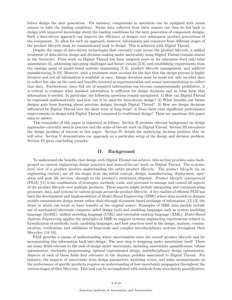
Of particular relevance is the process in which Digital Thread can be used in the design of the nextgeneration of products as illustrated in Figure 1. Here, multiple stages across the product lifecycle feed in-formation into the Digital Thread. Such information can be used to make informed choices on future designs,as well as to reduce uncertainty in design parameters and process costs. Additionally, such information mayuncover more efficient strategies for operation. Carrying out design decisions adds new information to theproduct lifecycle, changing the state of the Digital Thread. This whole process can be mathematically de-scribed with a data-driven design approach and decision problem under uncertainty. This paper formulatesthat mathematical description using the tools of Bayesian inference and decision theory.

Figure 1. Illustration of engineering design with Digital Thread.

To add context to this discussion, consider the design of a structural component where the operationalloads are uncertain. Practical approaches to deal with such uncertainty include over-conservative designs,damage tolerance policies, or redesigns and retrofits if analysis proves insufficient to ensure componentintegrity. Though the first generation of the component design may necessarily succumb to such practicalapproaches, data collected during the operational life of the first generation can be fed back and used to

2 of 21

American Institute of Aeronautics and Astronautics

better design the next generation. For instance, components in operation can be equipped with strainsensors to infer the loading conditions. Strain data collected from these sensors can then be fed back todesign with improved knowledge about the loading conditions for the next generation of component designs.Such a data-driven approach can improve the efficiency of designs over subsequent product generations ofthe component. To allow for such an approach, however, information and resources from different stages ofthe product lifecycle must be communicated back to design. This is achieved with Digital Thread.

Despite the range of data-driven technologies that currently exist across the product lifecycle, a unifiedtreatment of data-driven design and decision making under uncertainty using Digital Thread remains absentin the literature. Prior work on Digital Thread has been targeted more so for enterprise level risk/valueassessments [4], addressing upcoming challenges and future visions [5,6], and establishing requirements fromthe vantage point of model-based systems engineering [7, 8], product lifecycle management, and additivemanufacturing [9,10]. However, such a treatment must account for the fact that the design process is highlyiterative and not all information is available at once. Design decisions must be made not only on what datato collect but also on the costs and benefits involved in experimentation and sensor instrumentation to collectthat data. Furthermore, since full use of acquired information can become computationally prohibitive, itis critical to evaluate what minimal information is sufficient for design decisions and in what form thatinformation is needed. In particular, the following questions remain unexplored: 1) How can Digital Threadbe expressed mathematically and how can it be used for data-driven design? 2) What benefits can futuredesigns gain from learning about previous designs through Digital Thread? 3) How are design decisionsinfluenced by Digital Thread over the short term or long term? 4) Does there exist significant performanceimprovements in design with Digital Thread compared to traditional design? These are questions this paperaims to answer.

This remainder of this paper is organized as follows. Section II presents relevant background on designapproaches currently used in practice and the state-of-the-art work on Digital Thread. Section III introducesthe design problem of interest in this paper. Section IV details the underlying decision problem that wewill solve. Section V demonstrates our approach on a particular setup of the design and decision problem.Section VI gives concluding remarks.

II. Background

To understand the benefits that design with Digital Thread can achieve, this section provides some back-ground on current engineering design practices and state-of-the-art work on Digital Thread. The systems-level view of a product involves understanding the entire product lifecycle. The product lifecycle (in anengineering context) are all the stages from the initial concept, design, manufacturing, deployment, oper-ation and post life services, through to the product’s retirement/disposal. Product lifecycle management(PLM) [11] is the combination of strategies, methods, tools, and processes to manage and control all aspectsof the product lifecycle over multiple products. These aspects might include integrating and communicatingprocesses, data, and systems to various groups across the product lifecycle. A key enabler of efficient PLM hasbeen the development and implementation of Model-Based Engineering (MBE) where data models or domainmodels communicate design intent rather than through document-based exchange of information [12,13], thelatter in which can result in lossy transfer of the original source. Examples of MBE data models includeuse of mechanical/electronic computer aided design tools and modeling languages such as system modelinglanguage (SysML), unified modeling language (UML) and extensible markup language (XML). Model-BasedSystems Engineering applies the principles of MBE to support systems engineering requirements related toformalization of methods, tools, modeling languages, and best practices used in the design, analysis, commu-nication, verification, and validation of large-scale and complex interdisciplinary systems throughout theirlifecycles. [13–16].

PLM provides a means of understanding where uncertainties enter the overall product lifecycle and forincorporating this information back into design. The next step is designing under uncertainty itself. Thereare many fields relevant to the task of design under uncertainty, including uncertainty quantification, robustoptimization, stochastic programming, optimal experimental design, multidisciplinary design optimization.Aspects of each of these fields find relevance in the decision problem associated to Digital Thread. Forinstance, the impacts of uncertainty from design parameters, modeling errors, and noisy measurements onthe performance of specific products requires an understanding of how uncertainty propagates throughout thevarious stages of their lifecycles. This task can be accomplished with methods from uncertainty quantification,

3 of 21

American Institute of Aeronautics and Astronautics

which explores identification, characterization, and ultimately reduction of uncertainty of a simulation orphysical system [17]. In such systems, uncertainty quantification usually analyzes predicted outputs orspecific quantifies of interest [17], often (but not always) representing uncertainty via a probabilistic model.

Design decisions associated to Digital Thread will be determined through minimizing some cost metricsubject to constraints. Given the uncertainty just discussed, optimization methods to solve this problem willbe inherently stochastic based. Additionally, there are different ways to treat the stochastic optimizationproblem. One way is through robust optimization where a stochastic optimization problem is cast into adeterministic one through determining the maximum/minimum bounds of the sources of uncertainty andperforming an optimization over the range of these bounds [18]. Alternatively, stochastic programming treatsthe uncertainty with probabilistic models and optimization is performed on an objective statement (andpossibly constraints) involving some mean, variance, or other probabilistic criteria [19]. Uncertainty-basedmultidisciplinary design optimization methods seek to include considerations of reliability and robustness ina system-level design formulation [20–22].

To be able to design over multiple product generations, design decisions must be made not just oncurrent knowledge but also on potential future information. For instance, learning from operational datawill require deciding if the current generation of products should be designed to help improve future collectionof measurements (e.g., through optimally placed sensors or tailored structural architecture) or be designedonly to satisfy immediate metrics of performance. These design decisions will have to be guided throughsome metric of assessing benefits and costs. A field that explores this problem is optimal experimentaldesign (OED), where the objective is to determine experimental designs that are optimal with respect tosome statistical criteria or utility function [23]. In our context, experimental designs refer to actual designdecisions. Additionally, design decisions in the Digital Thread setting will be sequential in nature, wheredecisions of one generation will impact that of the next. This problem is explored in a sub-field of OEDknown as sequential optimal experimental design where experiments are conducted in sequence, and theresults of one experiment may affect the design of subsequent experiments [24].

In order to create a digital realization of more complicated components and systems, however, the DigitalThread must be able to account for information from data sources across multiple processes and disciplines.In recent efforts, methodologies such as Single Digital Thread Approach to Detailed Design (STAnDD) [25]work towards integrating multidisciplinary processes and analysis disciplines to more effectively evaluateproduct costs and performances. Additive manufacturing provides an additional opportunity to use Dig-ital Thread for integration of data-driven tools and physics-based simulations. In particular, use of theprinciples of Digital Thread in additive manufacturing has led to improvement in supply chain and pro-duction operations, reduction in time to design and manufacture parts, and decrease in manufactured partvariability [9]. Alternatively, improvements in manufacturing technology have allowed for exploring othermanufacturing strategies such as employing maintenance as part of a product’s standard lifecycle to minimizeoverall costs [26].

A relatively recent opportunity that motivates Digital Thread is the concept of an “attritable” vehicle,where the prospect of manufacturing and deploying small unmanned aerial vehicles at much lower costsopens up an opportunity for design to incorporate information gained through operational data (structuralstrains, air measurements, flight paths, energy consumption, payload history, and other related quantities)collected from sensors on-board the vehicles. Some use cases of attritable vehicles have been explored with theRevolutionary Affordable Architecture Generation and Evaluation (RAAGE) [27] framework where design,operations, manufacturing, and costs are integrated to enable rapid exploration of different cost-reducingdesigns and strategies.

III. Design Problem

This section describes the design problem considered in this paper and defines the elements of the designproblem along with their mathematical models.

III.A. Design Problem Description

We develop and illustrate our methodology in the context of a specific design problem, although the formu-lation is general and applies broadly across design problems. We consider a composite tow-steered (fiber-steered) planar component, where our objectives are to find the optimal fiber-steering and optimal component

4 of 21

American Institute of Aeronautics and Astronautics

thickness subject to the design and constraint metrics. This component may be, for example, a small systemsbracket on a larger assembly, a structural panel, or an aerodynamic control surface. In this paper, we explorethe specific example of the design of a chord-wise rib within a wing box section.

A challenge to our design task is the presence of uncertain input variables that will directly influencethe design of the product. In this problem specifically, the uncertain inputs are the loading the componentwill experience in operation, the material properties of the component, and the specific manufacturingtimestamps. Situations where these variables have most relevance is during the early stage of design, whentesting and experimentation have yet not taken place or when a brand new product is brought to market forwhich only partial design information can be used from other sources due to its novelty.

Large uncertainties in these inputs can lead to conservative designs that can be costly both to manufactureand operate. Thus, our goal is to collect data to reduce these uncertainties and thus to minimize costs.We can collect data through three different paths: Material properties can be learned through collection ofmeasurements from coupon level experiments; manufacturing timestamps can be learned from a combinationof a bill of materials, timestamps of individual processes, and other related documentation when a prototypeor product is manufactured; and operating loads can be learned from strain sensors placed on the productin operation.

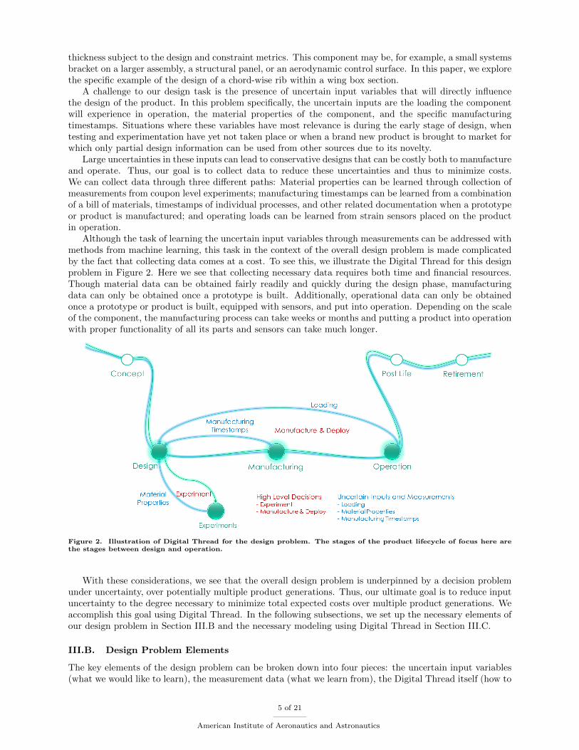
Although the task of learning the uncertain input variables through measurements can be addressed withmethods from machine learning, this task in the context of the overall design problem is made complicatedby the fact that collecting data comes at a cost. To see this, we illustrate the Digital Thread for this designproblem in Figure 2. Here we see that collecting necessary data requires both time and financial resources.Though material data can be obtained fairly readily and quickly during the design phase, manufacturingdata can only be obtained once a prototype is built. Additionally, operational data can only be obtainedonce a prototype or product is built, equipped with sensors, and put into operation. Depending on the scaleof the component, the manufacturing process can take weeks or months and putting a product into operationwith proper functionality of all its parts and sensors can take much longer.

Figure 2. Illustration of Digital Thread for the design problem. The stages of the product lifecycle of focus here arethe stages between design and operation.

With these considerations, we see that the overall design problem is underpinned by a decision problemunder uncertainty, over potentially multiple product generations. Thus, our ultimate goal is to reduce inputuncertainty to the degree necessary to minimize total expected costs over multiple product generations. Weaccomplish this goal using Digital Thread. In the following subsections, we set up the necessary elements ofour design problem in Section III.B and the necessary modeling using Digital Thread in Section III.C.

III.B. Design Problem Elements

The key elements of the design problem can be broken down into four pieces: the uncertain input variables(what we would like to learn), the measurement data (what we learn from), the Digital Thread itself (how to

5 of 21

American Institute of Aeronautics and Astronautics

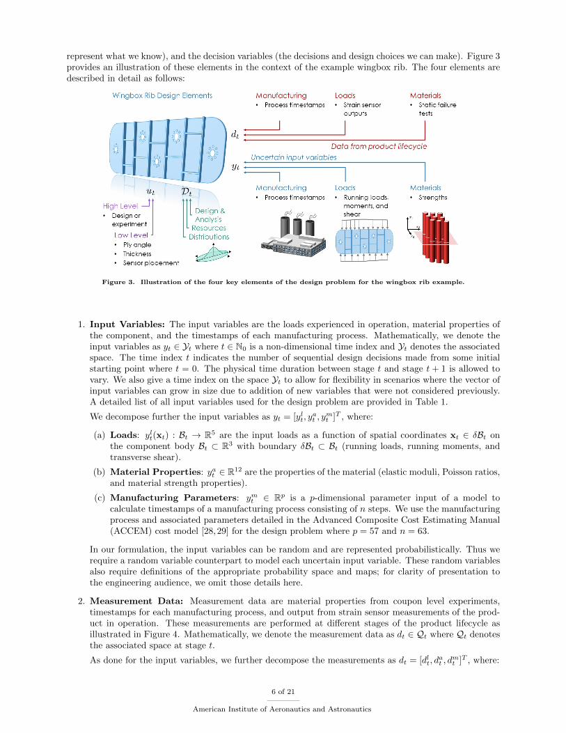
represent what we know), and the decision variables (the decisions and design choices we can make). Figure 3provides an illustration of these elements in the context of the example wingbox rib. The four elements aredescribed in detail as follows:

Figure 3. Illustration of the four key elements of the design problem for the wingbox rib example.

1. Input Variables: The input variables are the loads experienced in operation, material properties ofthe component, and the timestamps of each manufacturing process. Mathematically, we denote theinput variables as yt ∈ Yt where t ∈ N0 is a non-dimensional time index and Yt denotes the associatedspace. The time index t indicates the number of sequential design decisions made from some initialstarting point where t = 0. The physical time duration between stage t and stage t + 1 is allowed tovary. We also give a time index on the space Yt to allow for flexibility in scenarios where the vector ofinput variables can grow in size due to addition of new variables that were not considered previously.A detailed list of all input variables used for the design problem are provided in Table 1.

We decompose further the input variables as yt = [ylt, yat , y

mt ]T , where:

(a) Loads: ylt(xt) : Bt → R5 are the input loads as a function of spatial coordinates xt ∈ δBt onthe component body Bt ⊂ R3 with boundary δBt ⊂ Bt (running loads, running moments, andtransverse shear).

(b) Material Properties: yat ∈ R12 are the properties of the material (elastic moduli, Poisson ratios,and material strength properties).

(c) Manufacturing Parameters: ymt ∈ Rp is a p-dimensional parameter input of a model tocalculate timestamps of a manufacturing process consisting of n steps. We use the manufacturingprocess and associated parameters detailed in the Advanced Composite Cost Estimating Manual(ACCEM) cost model [28,29] for the design problem where p = 57 and n = 63.

In our formulation, the input variables can be random and are represented probabilistically. Thus werequire a random variable counterpart to model each uncertain input variable. These random variablesalso require definitions of the appropriate probability space and maps; for clarity of presentation tothe engineering audience, we omit those details here.

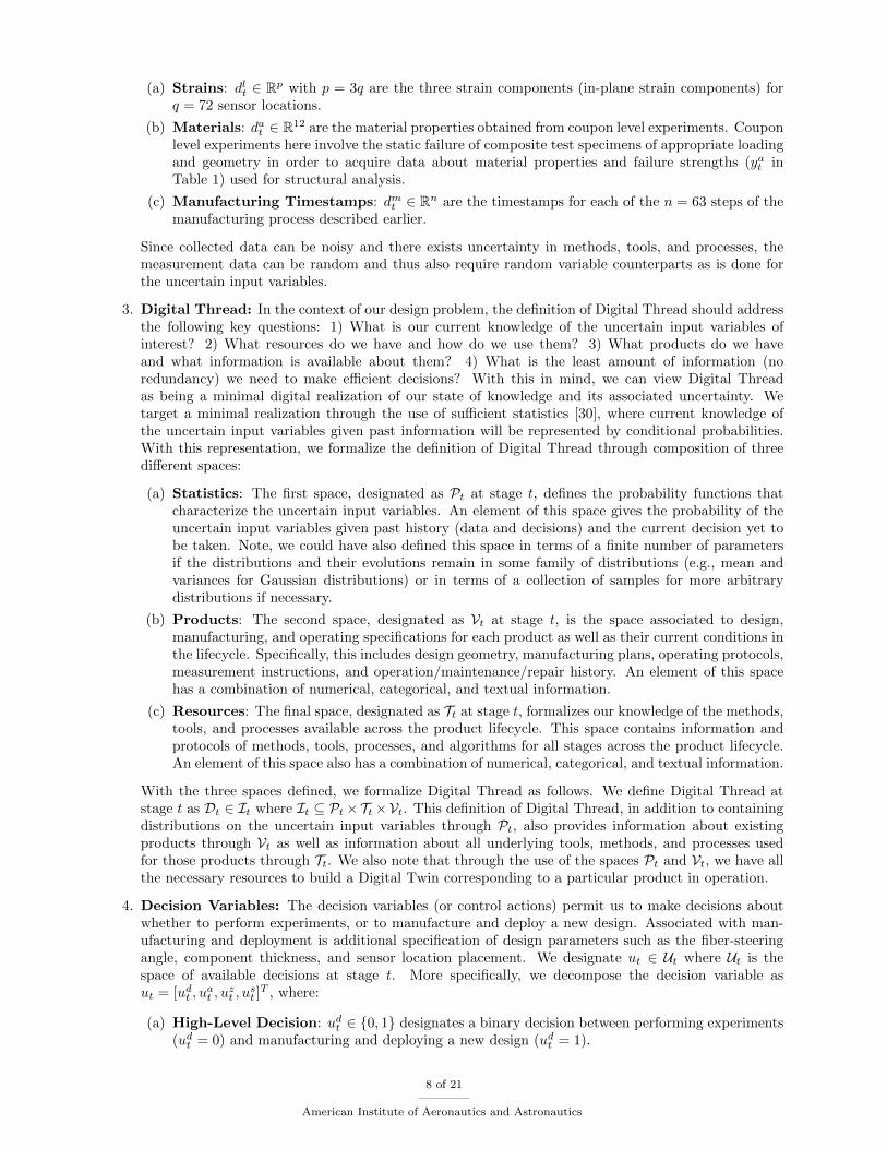
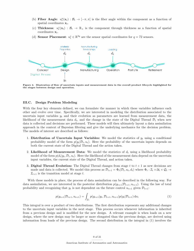
2. Measurement Data: Measurement data are material properties from coupon level experiments,timestamps for each manufacturing process, and output from strain sensor measurements of the prod-uct in operation. These measurements are performed at different stages of the product lifecycle asillustrated in Figure 4. Mathematically, we denote the measurement data as dt ∈ Qt where Qt denotesthe associated space at stage t.

As done for the input variables, we further decompose the measurements as dt = [dlt, dat , d

mt ]T , where:

6 of 21

American Institute of Aeronautics and Astronautics

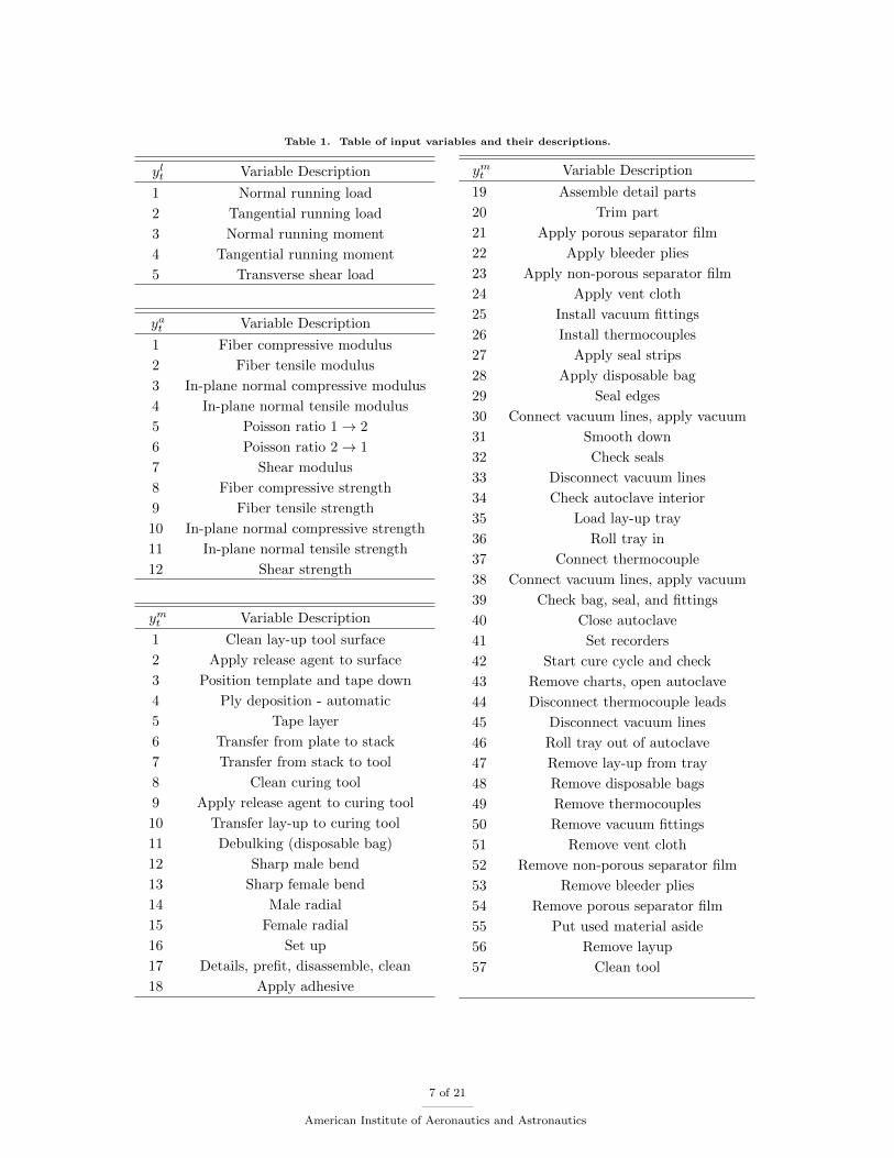
Table 1. Table of input variables and their descriptions.

ylt Variable Description

1 Normal running load

2 Tangential running load

3 Normal running moment

4 Tangential running moment

5 Transverse shear load

yat Variable Description

1 Fiber compressive modulus

2 Fiber tensile modulus

3 In-plane normal compressive modulus

4 In-plane normal tensile modulus

5 Poisson ratio 1→ 2

6 Poisson ratio 2→ 1

7 Shear modulus

8 Fiber compressive strength

9 Fiber tensile strength

10 In-plane normal compressive strength

11 In-plane normal tensile strength

12 Shear strength

ymt Variable Description

1 Clean lay-up tool surface

2 Apply release agent to surface

3 Position template and tape down

4 Ply deposition - automatic

5 Tape layer

6 Transfer from plate to stack

7 Transfer from stack to tool

8 Clean curing tool

9 Apply release agent to curing tool

10 Transfer lay-up to curing tool

11 Debulking (disposable bag)

12 Sharp male bend

13 Sharp female bend

14 Male radial

15 Female radial

16 Set up

17 Details, prefit, disassemble, clean

18 Apply adhesive

ymt Variable Description

19 Assemble detail parts

20 Trim part

21 Apply porous separator film

22 Apply bleeder plies

23 Apply non-porous separator film

24 Apply vent cloth

25 Install vacuum fittings

26 Install thermocouples

27 Apply seal strips

28 Apply disposable bag

29 Seal edges

30 Connect vacuum lines, apply vacuum

31 Smooth down

32 Check seals

33 Disconnect vacuum lines

34 Check autoclave interior

35 Load lay-up tray

36 Roll tray in

37 Connect thermocouple

38 Connect vacuum lines, apply vacuum

39 Check bag, seal, and fittings

40 Close autoclave

41 Set recorders

42 Start cure cycle and check

43 Remove charts, open autoclave

44 Disconnect thermocouple leads

45 Disconnect vacuum lines

46 Roll tray out of autoclave

47 Remove lay-up from tray

48 Remove disposable bags

49 Remove thermocouples

50 Remove vacuum fittings

51 Remove vent cloth

52 Remove non-porous separator film

53 Remove bleeder plies

54 Remove porous separator film

55 Put used material aside

56 Remove layup

57 Clean tool

7 of 21

American Institute of Aeronautics and Astronautics

(a) Strains: dlt ∈ Rp with p = 3q are the three strain components (in-plane strain components) forq = 72 sensor locations.

(b) Materials: dat ∈ R12 are the material properties obtained from coupon level experiments. Couponlevel experiments here involve the static failure of composite test specimens of appropriate loadingand geometry in order to acquire data about material properties and failure strengths (yat inTable 1) used for structural analysis.

(c) Manufacturing Timestamps: dmt ∈ Rn are the timestamps for each of the n = 63 steps of themanufacturing process described earlier.

Since collected data can be noisy and there exists uncertainty in methods, tools, and processes, themeasurement data can be random and thus also require random variable counterparts as is done forthe uncertain input variables.

3. Digital Thread: In the context of our design problem, the definition of Digital Thread should addressthe following key questions: 1) What is our current knowledge of the uncertain input variables ofinterest? 2) What resources do we have and how do we use them? 3) What products do we haveand what information is available about them? 4) What is the least amount of information (noredundancy) we need to make efficient decisions? With this in mind, we can view Digital Threadas being a minimal digital realization of our state of knowledge and its associated uncertainty. Wetarget a minimal realization through the use of sufficient statistics [30], where current knowledge ofthe uncertain input variables given past information will be represented by conditional probabilities.With this representation, we formalize the definition of Digital Thread through composition of threedifferent spaces:

(a) Statistics: The first space, designated as Pt at stage t, defines the probability functions thatcharacterize the uncertain input variables. An element of this space gives the probability of theuncertain input variables given past history (data and decisions) and the current decision yet tobe taken. Note, we could have also defined this space in terms of a finite number of parametersif the distributions and their evolutions remain in some family of distributions (e.g., mean andvariances for Gaussian distributions) or in terms of a collection of samples for more arbitrarydistributions if necessary.

(b) Products: The second space, designated as Vt at stage t, is the space associated to design,manufacturing, and operating specifications for each product as well as their current conditions inthe lifecycle. Specifically, this includes design geometry, manufacturing plans, operating protocols,measurement instructions, and operation/maintenance/repair history. An element of this spacehas a combination of numerical, categorical, and textual information.

(c) Resources: The final space, designated as Tt at stage t, formalizes our knowledge of the methods,tools, and processes available across the product lifecycle. This space contains information andprotocols of methods, tools, processes, and algorithms for all stages across the product lifecycle.An element of this space also has a combination of numerical, categorical, and textual information.

With the three spaces defined, we formalize Digital Thread as follows. We define Digital Thread atstage t as Dt ∈ It where It ⊆ Pt×Tt×Vt. This definition of Digital Thread, in addition to containingdistributions on the uncertain input variables through Pt, also provides information about existingproducts through Vt as well as information about all underlying tools, methods, and processes usedfor those products through Tt. We also note that through the use of the spaces Pt and Vt, we have allthe necessary resources to build a Digital Twin corresponding to a particular product in operation.

4. Decision Variables: The decision variables (or control actions) permit us to make decisions aboutwhether to perform experiments, or to manufacture and deploy a new design. Associated with man-ufacturing and deployment is additional specification of design parameters such as the fiber-steeringangle, component thickness, and sensor location placement. We designate ut ∈ Ut where Ut is thespace of available decisions at stage t. More specifically, we decompose the decision variable asut = [udt , u

at , u

zt , u

st ]T , where:

(a) High-Level Decision: udt ∈ {0, 1} designates a binary decision between performing experiments(udt = 0) and manufacturing and deploying a new design (udt = 1).

8 of 21

American Institute of Aeronautics and Astronautics

(b) Fiber Angle: uat (xt) : Bt → [−π, π] is the fiber angle within the component as a function ofspatial coordinates xt.

(c) Thickness: uzt (xt) : Bt → R+ is the component through thickness as a function of spatialcoordinates xt.

(d) Sensor Placement: ust ∈ R3q are the sensor spatial coordinates for q = 72 sensors.

Figure 4. Illustration of flow of uncertain inputs and measurement data in the overall product lifecycle highlighted forthe stages between design and operation.

III.C. Design Problem Modeling

With the four key elements defined, we can formulate the manner in which these variables influence eachother and evolve over time. Specifically, we are interested in modeling the distribution associated to theuncertain input variables yt and their evolution as parameters are learned from measurement data, thelikelihood of the measurement data dt, and the change in the state of the Digital Thread Dt when newdata is collected and decisions are performed. These models will then ultimately layout a data assimilationapproach in the context of Bayesian filtering and give the underlying mechanics for the decision problem.The models of interest are described as follows:

1. Distribution of Uncertain Input Variables: We model the statistics of yt using a conditionalprobability model of the form p(yt|Dt, ut). Here the probability of the uncertain inputs depends onboth the current state of the Digital Thread and the action taken.

2. Likelihood of Measurement Data: We model the statistics of dt using a likelihood probabilitymodel of the form p(dt|yt,Dt, ut). Here the likelihood of the measurement data depend on the uncertaininput variables, the current state of the Digital Thread, and action taken.

3. Digital Thread Evolution: The Digital Thread changes from stage t to t + 1 as new decisions aremade and data is collected. We model this process as Dt+1 = Φt(Dt, ut, dt) where Φt : It ×Ut ×Qt →It+1 is the transition model at stage t.

With these models in place, the process of data assimilation can be described in the following way. Fordata assimilation, we are interested in the posterior distribution p(yt+1|Dt+1, ut+1). Using the law of totalprobability and recognizing that yt is not dependent on the future control ut+1 given Dt+1:

p(yt+1|Dt+1, ut+1) =

∫Yt

p(yt+1|yt,Dt+1, ut+1)p(yt|Dt+1) dνt (1)

This integral is over a product of two distributions. The first distribution represents any additional changesto the uncertain input variables in the next stage. This process occurs whenever information is inheritedfrom a previous design and is modified for the new design. A relevant example is when loads on a newdesign, where the new design may be larger or more elongated than the previous design, are derived usinginformation from loads of the previous design. The second distribution in the integral in (1) involves the

9 of 21

American Institute of Aeronautics and Astronautics

actual data assimilation process. To see this, we use the fact that Dt+1 is by design a sufficient statistic forpast information (initial condition and measurement/control history) and Bayes rule to rewrite as:

p(yt|Dt+1) = p(yt|D0, u0, ..., ut, d0, ..., dt)

= p(yt|Dt, ut, dt)

=p(dt|yt,Dt, ut)p(yt|Dt, ut)

p(dt|Dt, ut)

(2)

which is just a product of the prior and likelihood models we presented earlier (with the appropriate normal-ization). Note, correlation of the inputs is handled automatically through an appropriate prior distributionon the inputs and conditional distributions p(yt|Dt, ut) and p(dt|yt,Dt, ut) used for the updates in (1).

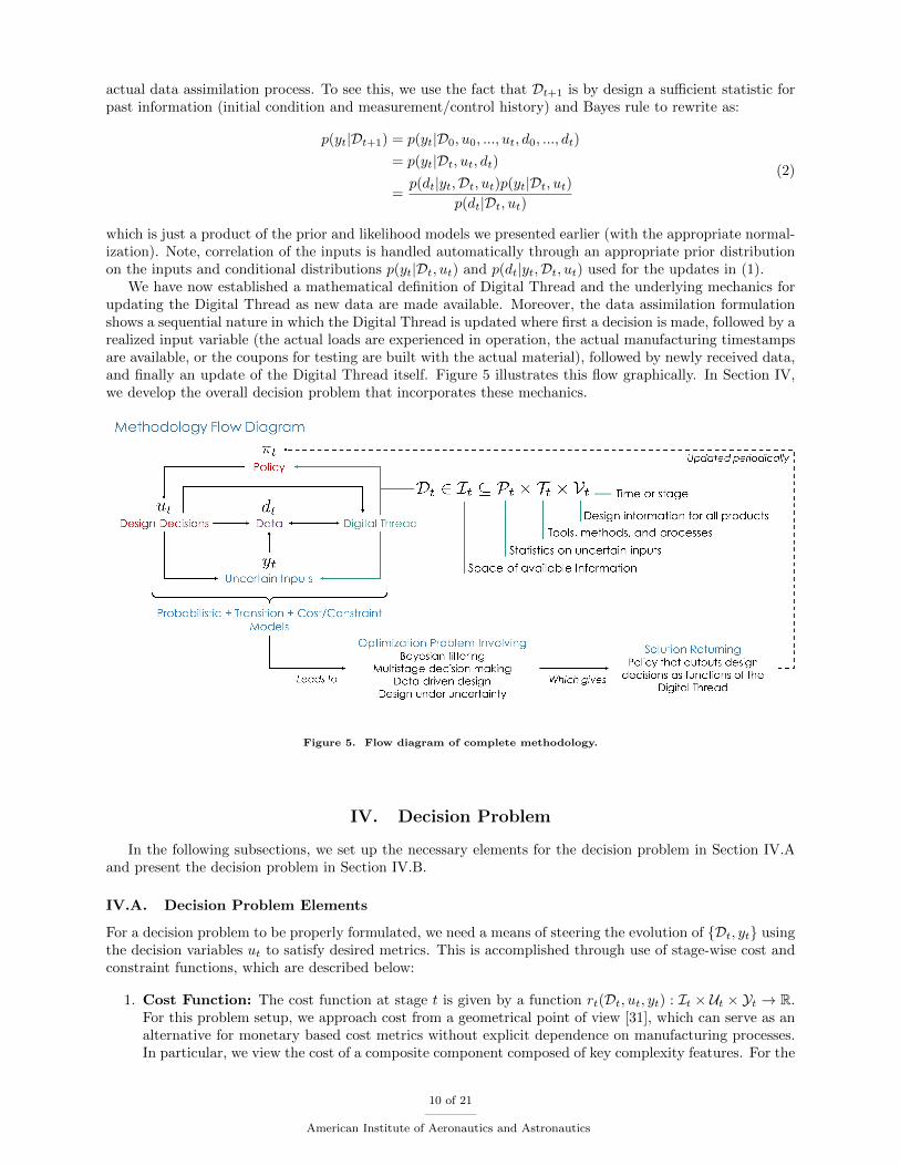
We have now established a mathematical definition of Digital Thread and the underlying mechanics forupdating the Digital Thread as new data are made available. Moreover, the data assimilation formulationshows a sequential nature in which the Digital Thread is updated where first a decision is made, followed by arealized input variable (the actual loads are experienced in operation, the actual manufacturing timestampsare available, or the coupons for testing are built with the actual material), followed by newly received data,and finally an update of the Digital Thread itself. Figure 5 illustrates this flow graphically. In Section IV,we develop the overall decision problem that incorporates these mechanics.

Figure 5. Flow diagram of complete methodology.

IV. Decision Problem

In the following subsections, we set up the necessary elements for the decision problem in Section IV.Aand present the decision problem in Section IV.B.

IV.A. Decision Problem Elements

For a decision problem to be properly formulated, we need a means of steering the evolution of {Dt, yt} usingthe decision variables ut to satisfy desired metrics. This is accomplished through use of stage-wise cost andconstraint functions, which are described below:

1. Cost Function: The cost function at stage t is given by a function rt(Dt, ut, yt) : It × Ut × Yt → R.For this problem setup, we approach cost from a geometrical point of view [31], which can serve as analternative for monetary based cost metrics without explicit dependence on manufacturing processes.In particular, we view the cost of a composite component composed of key complexity features. For the

10 of 21

American Institute of Aeronautics and Astronautics

design problem we explore N = 2 features related to fiber angle variation and component thickness.The two features have the following forms:

(a) Fiber Angle: We express complexity of the fiber angle as the norm squared of the fiber anglegradient divided by the thickness. In particular, let a fiber direction (angle) at some spatialcoordinate xt with through thickness uzt be described by uat . Then the feature associated withthat fiber angle is given by

ffibt (xt, ut) =

1

uzt (xt)||∇uat (xt)||22 (3)

where ffibt (xt, ut) : Bt×Ut → R+ is the feature associated to the fiber angle variation. The metric

here penalizes small thicknesses coupled with aggressive fiber angle changes and favors largerthicknesses with benign fiber angle changes. In addition, the metric favors straight in-plane fiberpaths. This metric is a small modification of the metric presented in Ref. 32.

(b) Component Thickness: We penalize two aspects of the component thickness: thickness vari-ation across the component body and overall volume. The feature associated with componentthickness uzt is given by

f thickt (xt, ut) = ||∇uzt (xt)||22 + β (4)

where f thickt (xt, ut) : Bt×Ut → R+ is the feature associated to the thickness variation and β ∈ R+

scales the penalty associated with total volume.

The complexity associated to each feature is given by an integration of that feature over the componentbody Bt:

Ifibt (ut) =

∫Bt

ffibt (xt, ut) dvt

Ithickt (ut) =

∫Bt

f thickt (xt, ut) dvt

(5)

The total complexity is given by an additive model of the form:

Itotalt (ut) = cfib

t Ifibt (ut) + cthick

t Ithickt (ut) (6)

for some weighting coefficients cfibt , c

thickt ∈ R+. The cost function is then given as rt(Dt, ut, yt) =

Itotalt (ut).

2. Constraint Function: The constraint function at stage t is given by a function gt(Dt, ut, yt) : It ×Ut×Yt → R. The constraint function we use is based on structural failure criteria. An arbitrary failurecriteria for structural analysis can be put in the form Fmt (σ, ε, yat ) where (in Voigt notation) σ ∈ R6

denotes a stress tensor, ε ∈ R6 denotes a strain tensor, and m denotes the mth mode of M total failuremodes. This expression is local and denotes the failure index at spatial coordinate xt. Failure occurswhenever Fmt (·) > 1. The constraint function is then given by a maximization over spatial coordinateson the component body and failure mode:

gt(Dt, ut, yt) = maxxt∈Bt,m∈[1,...,M ]

Fmt (σ(xt, ut, yt), ε(xt, ut, yt), yat )− 1 (7)

We investigate the Tsai-Wu criteria [33] as the failure metric. For the composite structural model, weuse the small displacement Mindlin-Reissner plate formulation [34,35] specialized for composites.

IV.B. Decision Problem Formulation

In setting up the decision problem, we would like to obtain answers to the following set of questions: Doesone invest early in small scale experiments to reduce the uncertainties for a subset of the uncertain inputvariables? Or does one proceed to manufacturing and deployment to gain revenue through sales and gatherother sources of data including specific manufacturing timestamps and operating conditions? When is onedecision favored over the other and under what conditions?

11 of 21

American Institute of Aeronautics and Astronautics

With all the ingredients in hand and motivations discussed, we formulate the decision problem in thefollowing way. We aim to minimize the expected total cost over a finite horizon (multiple product generations)subject to the immediate design constraints at stage t. Mathematically, this takes the form:

V ∗t (D′t) = minπt

E[ T∑k=t

γk−trk(Dk, µk, yk)|Dt = D′t, πt]

s.t. E[gt(Dt, µt, yt)|Dt = D′t, πt

]≤ 0, t ∈ {0, ..., T}

(8)

where a policy πt = {µt, ..., µT } defines a sequence of functions over the horizon T from time t. Each functionµt returns the control action ut, i.e. µt(·) = ut. Here, V ∗t (Dt) : It → R is the optimal value function orcost-to-go for Digital Thread Dt at stage t. The parameter γ ∈ [0, 1) is a discount factor. The expectationis taken over the uncertain inputs {yt, ..., yT } and measurement data {dt, ..., dT } with respect to the jointprobability distribution p(·|Dt = D′t, πt). Given the recursive structure of the decision statement, the optimalcost can be expressed in terms of the following Bellman Equation using Bellman’s principle of optimality [30]:

V ∗t (Dt) = minut∈Ut

E[rt(Dt, ut, yt) + γV ∗t+1(Φt(Dt, ut, dt))|Dt, ut

]s.t. E

[gt(Dt, ut, yt)|Dt, ut

]≤ 0, t ∈ {0, ..., T}, V ∗T+1 = 0

(9)

The solution to this dynamic program yields an optimal policy π∗t that specifies new designs and changes tothe Digital Thread for each step t up to the horizon T . Each function µ∗t of the optimal policy is a functionof Dt (a feedback policy), i.e. π∗t = {µ∗t (Dt), ..., µ∗T (DT )}.

A summary flow diagram of the complete methodology is given in Figure 5.

V. Demonstration

This section demonstrates our methodology on a specific setup of the decision problem introduced inSection IV.B.

V.A. Design Geometry

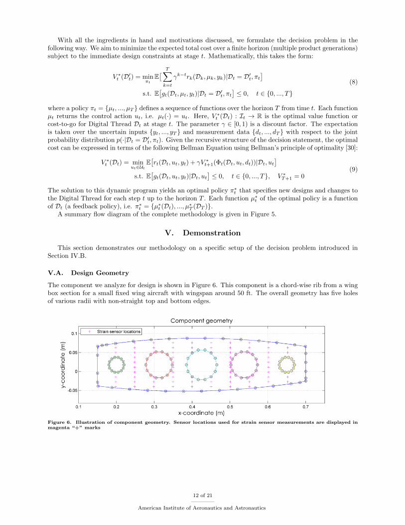
The component we analyze for design is shown in Figure 6. This component is a chord-wise rib from a wingbox section for a small fixed wing aircraft with wingspan around 50 ft. The overall geometry has five holesof various radii with non-straight top and bottom edges.

Figure 6. Illustration of component geometry. Sensor locations used for strain sensor measurements are displayed inmagenta “+” marks

12 of 21

American Institute of Aeronautics and Astronautics

V.B. Decision Problem of Interest

For the demonstration, we focus on the greedy version of the decision problem, where the discount factor isset to γ = 0. In this case the decision problem statement takes the simpler form:

V ∗t (Dt) = minut∈Ut

E[rt(Dt, ut, yt)|Dt, ut

]s.t. E

[gt(Dt, ut, yt)|Dt, ut

]≤ 0, t ∈ {0, ..., T}, V ∗T+1 = 0

(10)

Note, that in this particular setup the strategy of sensor placement is not present due to the absence of V ∗t+1,and hence dt, in the Bellman equation. That is, the policies that are generated are reactive to measurementsas opposed to having selection of where to best place sensors for the next design. This is because havingγ = 0 cancels out any contribution of future collected data in the optimization at each stage t. Non-zerodiscount factors will require solving the more general optimization problem given by (9).

To explore the behavior of design decisions on costs, we evaluate our formulation over three stagest ∈ {0, 1, 2} where we are allowed one set of coupon level experiments labeled with E (udt = 0), and twomanufacturing and deployments of a new design labeled with D (udt = 1). Enumerating these possibilitiesleads to two high-level decisions {EDD, DED} that we can take (the option DDE is excluded because it doesnot make sense to experiment after the products are already manufactured and deployed). For example,the sequence DED means to manufacture and deploy a new design first, followed by performing couponlevel experiments second, and the manufacturing and deploying another new design. The second designbenefits from data collected from both coupon experiments and operational measurements of the previousdesign. The two high-level decisions {EDD, DED} are distinguished by whether coupon experiments shouldbe performed first or second. Letting each high-level decision correspond to a specific policy, we have twopolicies to compare. Our methodology will assess which policy generates lower costs for the example problemin addition to returning specific designs for each policy.

Note, enumerating and assessing high level decisions as separate policies (e.g., EDD and DED) will scalecombinatorially based on the number of stages and high-level decisions available for each stage. However,in practice the number of high-level decisions of interest tend to be few for design-oriented objectives. Inaddition, the volatile nature of engineering design can bring upon new scenarios, objectives, and problemrestructuring that can not all be accounted for practically in an optimization of a past stage. Thus, thenumber of stages to be evaluated will also be few. Reduction in computational time for a large number ofpolices can be achieved by updating and evaluating policies in parallel if necessary.

V.C. Setup of Design Problem Elements

For the demonstration, data and statistical parameters are generated synthetically using computationalmodels and baseline loads information. The specific representation of the four elements are presented in thefollowing:

1. Uncertain Input Variables: We model the uncertain input variables using Gaussian random vari-ables with specified initial means and covariances. The small displacement Mindlin-Reissner platemodel gives a linear mapping between loads and strain measurements, the map from material propertiesto measured material properties using coupon experiments is linear, and the map from manufacturingparameters to manufacturing timestamps is setup to be linear for this particular demonstration; thus,the uncertain input variables remains Gaussian over subsequent stages t.

2. Measurement Data: We model the measurement data using the aforementioned linear models thatmap input variables to measurement data with additive Gaussian noise. Strain sensor placement isassumed fixed for this demonstration.

3. Digital Thread: In this case, the Digital Thread comprises the distributions on the uncertain inputvariables as well as parameters and labels for the particular finite element solver and failure crite-ria, the noise parameters of the measurements, design geometry for components in operation, andcost/constraint parameters. The distributions on the uncertain input variables are calculated usingKalman Filters with the prediction and analyze steps reversed, as prescribed by the Bayesian filter in(1).

13 of 21

American Institute of Aeronautics and Astronautics

4. Decision Variables: The decision problem is solved using a policy parametrization technique. Sincethe ply angle and thickness are spatial in nature while the Digital Thread lives in information space, thepolicy parametrization will involve functions over both Bt and It. In particular, the low-level controlis determined using the following parametrization of the policy:

µat (xt,Dt) =

K∑k=1

L∑l=1

ψkt (xt)Aklt φ

lt(Dt)

µzt (xt,Dt) =

K∑k=1

L∑l=1

ψkt (xt)Zklt φ

lt(Dt)

µst = [x1t , ...,x

qt ]T

(11)

where Aklt , Zklt ∈ R are the policy parametrization matrix coefficients for ply angle and thickness,

respectively. Here, ψkt (xt) : Bt → R is the kth basis function over spatial points on the componentbody Bt and φlt(Dt) : It → R is the lth basis function over features of the Digital Thread Dt ininformation space It. The features of the Digital Thread used here are the means and variances of theuncertain input variables extracted from the Digital Thread. The basis functions over spatial pointson the body are expressed using Gaussian radial basis functions where the arguments are pre-scaledto lie on the unit hypercube. We use K basis functions centered at K points over spatial coordinates,where the centers of the radial basis functions correspond to the nodes of the finite element model.The basis functions over the features of the Digital Thread are expressed using L monomials.

The parametrizations in (11) are then optimized using a policy gradient method [36, 37] applied tothe decision statement (10). Expectations in (10) are approximated using Monte Carlo simulations.Monte Carlo errors are estimated numerically. We determined that approximately 100 samples weresufficient to ensure errors in the Monte Carlo approximations of the expectations in (10) were within2%, based on numerically estimated statistics of rt(·) for feasible designs.

Other modeling choices for the setup: At stage 0, the Digital Thread starts with large uncertaintiesin both the input loadings and material strength properties. The input loadings known at stage 0 havea mean that is 1.5 times larger than the mean of the input loadings the component will actually see inoperation. The material strength properties known at stage 0 have means 0.9 times that of the actualmaterial strength properties. The material moduli and Poisson ratios are assumed fixed and known. Weset the operating costs to be 0.05 times the costs of manufacturing and deploying of the component. Datacan be collected from manufacturing to operation only after a design has been manufactured and deployedfrom a previous time step. Costs to perform coupon level experiments are assumed negligible in comparisonto other costs for this particular setup. The scalars in the cost model specified in (4) and (6) are set toβ = 0.001, cfib

t = 0.2, and cthickt = 105.

V.D. Results

In Figure 7, we show the typical effect of updating our knowledge of the uncertain loads by learning from thedata collected from strain sensor measurements after deployment of a design. Here, the loads used for theinitial design are compared to the loads estimated from operational data of the previously deployed design.These estimated loads are then used for the second design. The mean and two standard deviations of thevariance for the initial estimate of loads (before any data assimilation) are shown with the red dashed-dottedline and red shading, respectively. Similarly, the mean and two standard deviations of the variance forthe estimate of the loads after a design is deployed are shown with the blue dashed line and blue shading,respectively. The actual loads to be learned are shown with the thick magenta line. The large shifts inthe mean and variance reduction of the running loads and normal running moment after data assimilationindicate that the design of the next generation can be built lighter (and therefore at a lower cost) than theprevious generation. This is because the loads for this example setup are learned to be of lesser magnitudethan what was used for the design of the previous generation. However, in order to have obtained thisknowledge, we had to deploy a design in the first place—and that has a cost.

14 of 21

American Institute of Aeronautics and Astronautics

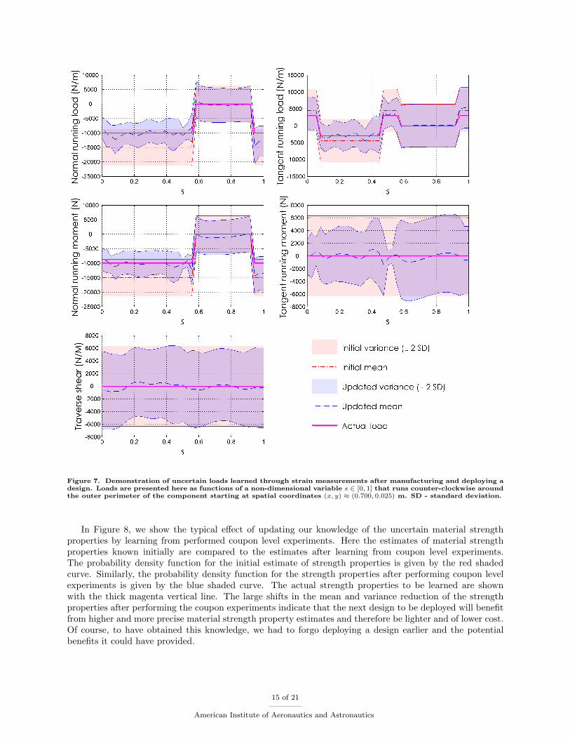
Figure 7. Demonstration of uncertain loads learned through strain measurements after manufacturing and deploying adesign. Loads are presented here as functions of a non-dimensional variable s ∈ [0, 1] that runs counter-clockwise aroundthe outer perimeter of the component starting at spatial coordinates (x, y) ≈ (0.700, 0.025) m. SD - standard deviation.

In Figure 8, we show the typical effect of updating our knowledge of the uncertain material strengthproperties by learning from performed coupon level experiments. Here the estimates of material strengthproperties known initially are compared to the estimates after learning from coupon level experiments.The probability density function for the initial estimate of strength properties is given by the red shadedcurve. Similarly, the probability density function for the strength properties after performing coupon levelexperiments is given by the blue shaded curve. The actual strength properties to be learned are shownwith the thick magenta vertical line. The large shifts in the mean and variance reduction of the strengthproperties after performing the coupon experiments indicate that the next design to be deployed will benefitfrom higher and more precise material strength property estimates and therefore be lighter and of lower cost.Of course, to have obtained this knowledge, we had to forgo deploying a design earlier and the potentialbenefits it could have provided.

15 of 21

American Institute of Aeronautics and Astronautics

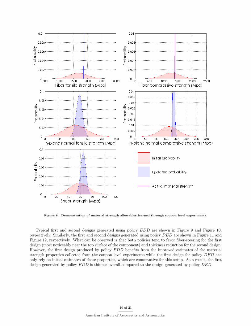
Figure 8. Demonstration of material strength allowables learned through coupon level experiments.

Typical first and second designs generated using policy EDD are shown in Figure 9 and Figure 10,respectively. Similarly, the first and second designs generated using policy DED are shown in Figure 11 andFigure 12, respectively. What can be observed is that both policies tend to favor fiber-steering for the firstdesign (most noticeably near the top surface of the component) and thickness reduction for the second design.However, the first design produced by policy EDD benefits from the improved estimates of the materialstrength properties collected from the coupon level experiments while the first design for policy DED canonly rely on initial estimates of those properties, which are conservative for this setup. As a result, the firstdesign generated by policy EDD is thinner overall compared to the design generated by policy DED.

16 of 21

American Institute of Aeronautics and Astronautics

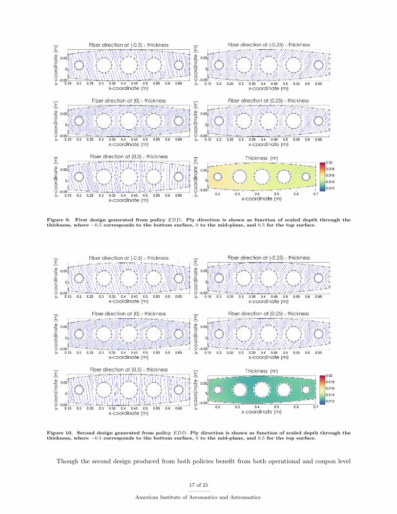
Figure 9. First design generated from policy EDD. Ply direction is shown as function of scaled depth through thethickness, where −0.5 corresponds to the bottom surface, 0 to the mid-plane, and 0.5 for the top surface.

Figure 10. Second design generated from policy EDD. Ply direction is shown as function of scaled depth through thethickness, where −0.5 corresponds to the bottom surface, 0 to the mid-plane, and 0.5 for the top surface.

Though the second design produced from both policies benefit from both operational and coupon level

17 of 21

American Institute of Aeronautics and Astronautics

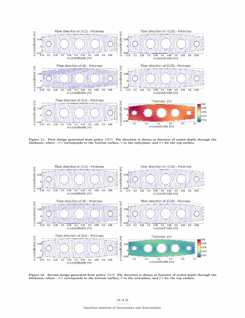
Figure 11. First design generated from policy DED. Ply direction is shown as function of scaled depth through thethickness, where −0.5 corresponds to the bottom surface, 0 to the mid-plane, and 0.5 for the top surface.

Figure 12. Second design generated from policy DED. Ply direction is shown as function of scaled depth through thethickness, where −0.5 corresponds to the bottom surface, 0 to the mid-plane, and 0.5 for the top surface.

18 of 21

American Institute of Aeronautics and Astronautics

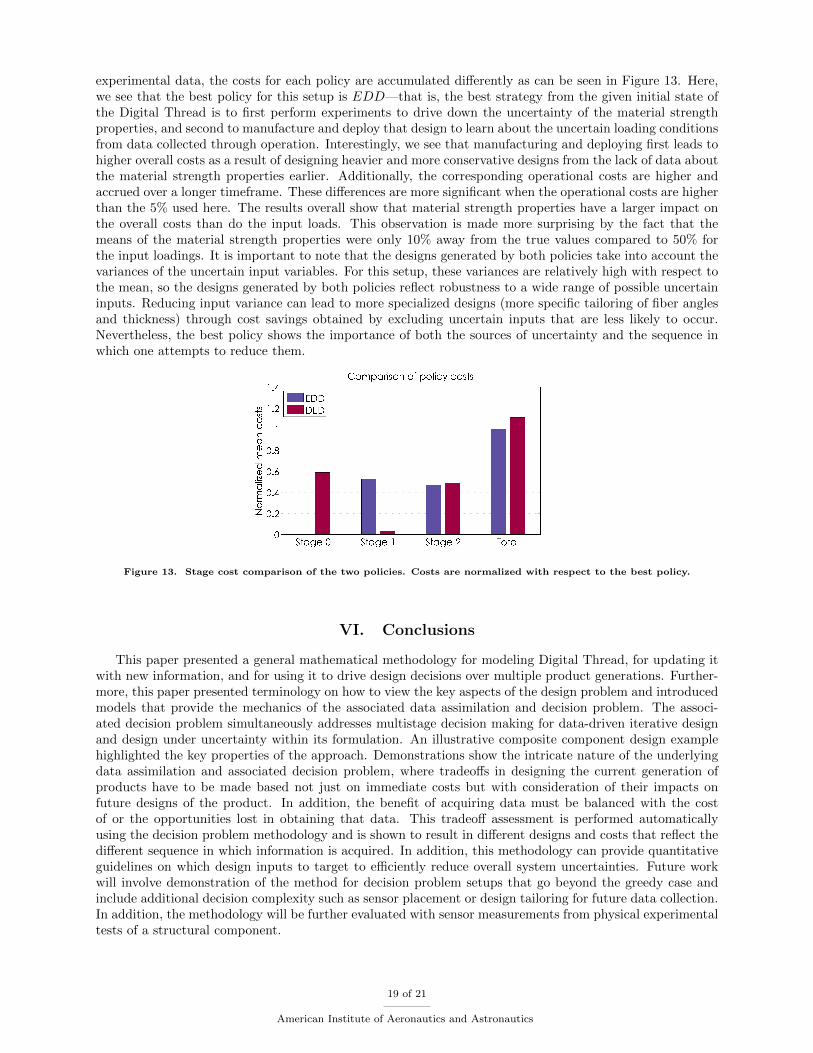
experimental data, the costs for each policy are accumulated differently as can be seen in Figure 13. Here,we see that the best policy for this setup is EDD—that is, the best strategy from the given initial state ofthe Digital Thread is to first perform experiments to drive down the uncertainty of the material strengthproperties, and second to manufacture and deploy that design to learn about the uncertain loading conditionsfrom data collected through operation. Interestingly, we see that manufacturing and deploying first leads tohigher overall costs as a result of designing heavier and more conservative designs from the lack of data aboutthe material strength properties earlier. Additionally, the corresponding operational costs are higher andaccrued over a longer timeframe. These differences are more significant when the operational costs are higherthan the 5% used here. The results overall show that material strength properties have a larger impact onthe overall costs than do the input loads. This observation is made more surprising by the fact that themeans of the material strength properties were only 10% away from the true values compared to 50% forthe input loadings. It is important to note that the designs generated by both policies take into account thevariances of the uncertain input variables. For this setup, these variances are relatively high with respect tothe mean, so the designs generated by both policies reflect robustness to a wide range of possible uncertaininputs. Reducing input variance can lead to more specialized designs (more specific tailoring of fiber anglesand thickness) through cost savings obtained by excluding uncertain inputs that are less likely to occur.Nevertheless, the best policy shows the importance of both the sources of uncertainty and the sequence inwhich one attempts to reduce them.

Figure 13. Stage cost comparison of the two policies. Costs are normalized with respect to the best policy.

VI. Conclusions

This paper presented a general mathematical methodology for modeling Digital Thread, for updating itwith new information, and for using it to drive design decisions over multiple product generations. Further-more, this paper presented terminology on how to view the key aspects of the design problem and introducedmodels that provide the mechanics of the associated data assimilation and decision problem. The associ-ated decision problem simultaneously addresses multistage decision making for data-driven iterative designand design under uncertainty within its formulation. An illustrative composite component design examplehighlighted the key properties of the approach. Demonstrations show the intricate nature of the underlyingdata assimilation and associated decision problem, where tradeoffs in designing the current generation ofproducts have to be made based not just on immediate costs but with consideration of their impacts onfuture designs of the product. In addition, the benefit of acquiring data must be balanced with the costof or the opportunities lost in obtaining that data. This tradeoff assessment is performed automaticallyusing the decision problem methodology and is shown to result in different designs and costs that reflect thedifferent sequence in which information is acquired. In addition, this methodology can provide quantitativeguidelines on which design inputs to target to efficiently reduce overall system uncertainties. Future workwill involve demonstration of the method for decision problem setups that go beyond the greedy case andinclude additional decision complexity such as sensor placement or design tailoring for future data collection.In addition, the methodology will be further evaluated with sensor measurements from physical experimentaltests of a structural component.

19 of 21

American Institute of Aeronautics and Astronautics

VII. Acknowledgements

This work is supported in part by AFOSR grant FA9550-16-1-0108 under the Dynamic Data DrivenApplication System Program (Program Manager Dr. E. Blasch), the MIT-SUTD International DesignCenter, and the United States Department of Energy Office of Advanced Scientific Computing Research(ASCR) grants DE-FG02-08ER2585 and DE-SC0009297, as part of the DiaMonD Multifaceted MathematicsIntegrated Capability Center (program manager Dr. S. Lee).

References

[1] US Airforce, Global Horizons Final Report: United States Air Force Global Science and Technology Vision - AF/STTR 13-01 , United States Air Force, 2013.

[2] Kraft, E., “HPCMP CREATE-AV and the Air Force Digital Thread,” in AIAA SciTech 2015, 53th AIAA AerospaceSciences Meeting, Kissimmee, Florida, 2015, pp. 1–13, doi:10.2514/6.2015-0042.

[3] West, T. and Pyster, A., “Untangling the Digital Thread: The Challenge and Promise of Model-Based Engineering inDefense Acquisition,” INSIGHT , Vol. 18, No. 2, 2015, pp. 45–55, doi:10.1002/inst.12022.

[4] Burgaud, F., Durand, J., and Mavris, D., “A Decision-Support Methodology to Make Enterprise-Level Risk/ValueTrade-Offs,” in AIAA SciTech 2017, 19th AIAA Non-Deterministic Approaches Conference, Grapevine, Texas, 2017, pp. 1–14,doi:10.2514/6.2017-0589.

[5] Kobryn, P., Tuegel, E., Zweber, J., and Kolonay, R., “Digital Thread and Twin for Systems Engeering: EMD to Dis-posal,” in AIAA SciTech 2017, 55th AIAA Aerospace Sciences Meeting, Grapevine, Texas, 2017, pp. 1–13, doi:10.2514/6.2017-0876.

[6] Zweber, J., Kolonay, R., Kobryn, P., and Tuegel, E., “Digital Thread and Twin for Systems Engeering: Pre-MDD through TMRR,” in AIAA SciTech 2017, 55th AIAA Aerospace Sciences Meeting, Grapevine, Texas, 2017, pp. 1–26,doi:10.2514/6.2017-0875.

[7] Hedberg, T., Lubell, J., Fischer, L., Maggiano, L., and Feeney, A., “Testing the Digital Thread in Support of Model-Based Manufacturing and Inspection,” Journal of Computing and Information Science in Engineering, Vol. 16, No. 2, 2016,doi:10.1115/1.4032697.

[8] Sundaram, V. and Brownlow, L., “MBSE Digital System Model for AF DCGS,” in AIAA SciTech 2018, 2018 AIAAAerospace Sciences Meeting, Kissimmee, Florida, 2018, pp. 1–17, doi:10.2514/6.2018-1217.

[9] Mies, D., Marsden, W., and Warde, S., “Overview of Additive Manufacturing Informatics: “A Digital Thread”,”Integrating Materials and Manufacturing Innovation, Vol. 5, No. 1, 2016, pp. 1–6, doi:10.1186/s40192-016-0050-7.

[10] Nassar, A. and Reutzel, E., “A proposed digital thread for additive manufacturing,” in International Solid FreeformFabrication Symposium, Austin, Texas, 2013.

[11] Stark, J., Product Lifecycle Management , Springer International, 2015, doi:10.1007/978-3-319-17440-2.

[12] Wymore, A., Model-Based Systems Engineering, CRC press, 1993.

[13] Ramos, A., Ferreira, J., and Barcelo, J., “Model-Based Systems Engineering: An Emerging Approach for ModernSystems,” IEEE Transactions on Systems,Man, and Cybernetics - Part C: Applications and Reviews, 2012, pp. 101–111,doi:10.1109/TSMCC.2011.2106495.

[14] Estefan, J., “MBSE Methodology Survey,” INSIGHT-INCOSE J., Vol. 12, No. 4, 2009, pp. 16–18,doi:10.1002/inst.200912416.

[15] Cloutier, R., “Introduction to this Special Edition on Model-Based Systems Engineering,” INSIGHT-INCOSE J.,Vol. 12, No. 4, 2009, pp. 7–8, doi:10.1002/inst.20091247.

[16] Holland, T., Modeling and Simulation in the Systems Engineering Life Cycle: Core Concepts and AccompanyingLectures, Springer-Verlag London, 2015, doi:10.1007/978-1-4471-5634-5.

[17] Smith, R., Uncertainty Quantification: Theory, Implementation, and Applications, SIAM Computational Science &Engineering, 2014.

[18] Bertsimas, D., Brown, D., and Caramanis, C., “Theory and Applications or Robust Optimization,” SIAM Review ,Vol. 53, No. 3, 2011, pp. 464–501, doi:10.1137/080734510.

[19] Kall, P., Wallace, S., and Kall, P., Stochastic Programming, John Wiley & Sons, Chichester, 1994.

[20] Yao, W., Chen, X., Luo, W., van Tooren, M., and Guo, J., “Review of uncertainty-based multidisciplinary de-sign optimization methods for aerospace vehicles,” Progress in Aerospace Science, Vol. 47, No. 6, 2011, pp. 450–479,doi:10.1016/j.paerosci.2011.05.001.

[21] Du, X. and Chen, W., “Efficient Uncertainty Analysis Methods for Multidisciplinary Robust Design,” AIAA Journal ,Vol. 40, No. 3, 2002, pp. 545–552, doi:10.2514/2.1681.

[22] Kokkolaras, M., Mourelatos, Z., and Papalambros, P., “Design Optimization of Hierarchically Decomposed MultilevelSystems Under Uncertainty,” ASME International Design Engineering Technical Conferences and Computers and Informationin Engineering Conference, Volume 1: 30th Design Automation Conference, 2004, pp. 613–624, doi:10.1115/DETC2004-57357.

[23] Atkinson, A., Donev, A., and Tobias, R., Optimum Experimental Designs, with SAS (Oxford Statistical ScienceSeries), Oxford University Press, 2007.

[24] Huan, X. and Marzouk, Y., “Simulation-based Optimal Bayesian Experimental Design for Nonlinear Systems,” Journalof Computational Physics, Vol. 232, No. 1, 2013, pp. 288–317, doi:10.1016/j.jcp.2012.08.013.

[25] Gharbi, A., Sarojini, D., Kallou, E., Harper, D., Petitgenet, V., Rancourt, D., Briceno, S., and Mavris, D., “STAnDD:A Single Digital Thread Approach to Detailed Design,” in AIAA SciTech 2017, 55th AIAA Aerospace Sciences Meeting,Grapevine, Texas, 2017, pp. 1–13, doi:10.2514/6.2017-0693.

20 of 21

American Institute of Aeronautics and Astronautics

[26] Thomsen, B., Kokkolaras, M., Mnsson, T., and Isaksson, O., “Quantitative Assessment of the Impact of AlternativeManufacturing Methods on Aeroengine Component Lifing Decisions,” ASME Journal of Mechanical Design, Vol. 139, No. 2,2016, pp. 021401–1–021401–10, doi:10.1115/1.4034883.

[27] Pagan, J., Huynh, D., Schafer, S., Pinon, O., and Mavris, D., “Revolutionary Affordable Architecture Generation &Evaluation - Application to a System of Attritable UAVs,” in AIAA SciTech 2018, 2018 AIAA Aerospace Sciences Meeting,Kissimmee, Florida, 2018, pp. 1–25, doi:10.2514/6.2018-1743.

[28] Gutowski, T., Hoult, D., Dillon, G., Neoh, E., Muter, S., E.Kim, and Tse, M., “Development of a Theoretical CostModel for Advanced Composite Fabrication,” Composites Manufacturing, Vol. 5, No. 4, 1994, pp. 231–239, doi:10.1016/0956-7143(94)90138-4.

[29] Corporation, N., “Advanced Composites Cost Estimating Manual (ACCEM),” AFFDL-TR-76-87 , 1976, pp. 1–80.

[30] Bertsekas, D., Dynamic Programming and Optimal Control , Vol. I, Athena Scientific, 3rd ed., 2005.

[31] Tse, M., Design Cost Model for Advanced Composite Structures, PhD Thesis, MIT, 1992.

[32] Brooks, T. and Martins, J., “High-fidelity Aerostructural Optimization of a High Aspect Ratio Tow-steered CompositeWing,” in AIAA SciTech 2016, 57th AIAA/ASCE/AHS/ASC Structures, Structural Dynamics, and Materials Conference,San Diego, CA, 2016, pp. 1–16, doi:10.2514/6.2016-1179.

[33] Tsai, S. and Wu, E., “A General Theory of Strength for Anisotropic Materials,” Journal of Composite Materials,1971, pp. 58–80, doi:10.1177/002199837100500106.

[34] Mindlin, R., “Influence of Rotatory Inertia and Shear on Flexural Motions of Isotropic, Elastic Plates,” ASME Journalof Applied Mechanics, 1951, pp. 31–38.

[35] Reissner, E., “The Effect of Transverse Shear Deformation on the Bending of Elastic Plates,” ASME Journal of AppliedMechanics, 1945, pp. A69–A77.

[36] Sutton, R., McAllester, D., Singh, S., and Mansour, Y., “Policy Gradient Methods for Reinforcement Learning withFunction Approximation,” In Advances in Neural Information Processing Systems, 2000, pp. 1057–1063.

[37] Kakade, S., “A Natural Policy Gradient,” In Advances in Neural Information Processing Systems, 2002, pp. 1531–1538.

21 of 21

American Institute of Aeronautics and Astronautics