FORSCHUNGSBERICHT AGRARTECHNIK des Fachausschusses Forschung und Lehre der

Max-Eyth-Gesellschaft Agrartechnik im VDI (VDI-MEG)

Franz Djamil Román Sufán

Experimental and CFD study on low temperature drying of loose and compressed bulks

Dissertation Witzenhausen 2014

539

Universität Kassel

Fachbereich Ökologische Agrarwissenschaften

Fachgebiet Agrartechnik

Prof. Dr. sc. agr. Oliver Hensel

Experimental and CFD study on low temperature drying of loose and compressed bulks

Dissertation zur Erlangung des akademischen Grades Doktor der Agrarwissenschaften (Dr. agr.)

von M.Sc. Franz Djamil Román Sufán

aus Lima, Perú

2014

Die vorliegende Arbeit wurde vom Fachbereich für Ökologische Agrarwissenschaften, Fachgebiet Agrartechnik der Universität Kassel als Dissertation zur Erlangung des akademischen Grades Doktor der Agrarwissenschaften angenommen. Tag der mündlichen Prüfung: 12.11.2014

Erster Gutachter: Prof. Dr. Oliver Hensel Zweiter Gutachter: Prof. Dr. Frank Beneke

Mündliche Prüfer: Prof. Dr. Michael Wachendorf Dr. Christian Krutzinna

Alle Rechte vorbehalten. Die Verwendung von Texten und Bildern, auch auszugsweise, ist ohne Zustimmung des Autors urheberrechtswidrig und strafbar. Das gilt insbesondere für Vervielfältigung, Übersetzung, Mikroverfilmung sowie die Einspeicherung und Verarbeitung in elektronischen Systemen.

© 2014

Im Selbstverlag: Franz Djamil Román Sufán

Bezugsquelle: Universität Kassel, FB Ökologische Agrarwissenschaften

Fachgebiet Agrartechnik

Nordbahnhofstr. 1a

37213 Witzenhausen

Preface

This thesis is submitted to the Faculty of Organic Agricultural Sciences of the University of Kassel to fulfill the requirements for the degree Doktor der Agrarwissenschaften (Dr. agr.). This dissertation is based on five papers as first author, which are published in, or submitted to, international refereed journals.

I want to thank Prof. Dr. Oliver Hensel for his invaluable guidance, support and encouragement, and for having always his door open for discussion and advice.

I also want to thank Prof. Dr. Frank Beneke for agreeing to assess this work, and Prof. Dr. Michael Wachendorf and Dr. Christian Krutzinna for their participation as oral examiners.

The friendly atmosphere at the Institute of Agricultural Engineering has been important for my work and I wish to thank my colleagues, especially Christian, Uwe and Heiko for their time as well as their technical and logistic support.

I also want to thank my parents who encouraged me to study abroad and have continued encouraging me from Perú all these years. Finally I thank my wife Nadine for her constant support and patience, her interest in my work, and for putting up with my occasional bad or strange mood.

List of papers

Parts of this thesis have been published or are submitted for publication as:

Chapter 3. Román, F., & Hensel, O. (2010). Sorption isotherms of celery leaves (Apium graveolens var. secalinum ). Agricultural Engineering International: CIGR Journal 12(3), 137-141.

Chapter 4. Román, F., & Hensel, O. (2011). Effect of air temperature and relative humidity on the thin-layer drying of celery leaves (Apium graveolens var. secalinum). Agricultural Engineering International: CIGR Journal 13(2).

Chapter 5. Román, F., Strahl-Schäfer, V., & Hensel, O. (2012). Improvement of air distribution in a fixed-bed dryer using computational fluid dynamics. Biosystems Engineering 112(4), 359-369.

Chapter 6. Román, F., & Hensel, O. (2014). Numerical simulations and experimental measurements on the distribution of air and drying of round hay bales. Biosystems Engineering 122, 1-15.

Chapter 7. Román, F., & Hensel, O. (2014). Real-time product moisture content monitoring in batch dryer using psychrometric and airflow measurements. Computers and Electronics in Agriculture 107, 97-103.

Table of contents

1 General introduction ............................................................................ 13

2 Objectives of the research ................................................................... 17

3 Sorption Isotherms of Celery Leaves ( Apium graveolens var. secalinum) ............................................................................................. 18

3.1 Introduction ......................................................................................................... 18

3.2 Materials and methods ....................................................................................... 18

3.2.1 Plant material ......................................................................................... 18

3.2.2 Experimental procedure ......................................................................... 19

3.2.3 Model fitting ............................................................................................ 20

3.3 Results and discussion ....................................................................................... 21

3.4 Conclusions ........................................................................................................ 24

4 Effect of air temperature and relative humidity on the thin-layer drying of celery leaves ( Apium graveolens var. secalinum) ............................................................................................. 25

4.1 Introduction ......................................................................................................... 25

4.2 Materials and Methods ....................................................................................... 26

4.2.1 Plant Material ......................................................................................... 26

4.2.2 Drying apparatus .................................................................................... 26

4.2.3 Experimental Procedure ......................................................................... 26

4.2.4 Model fitting ............................................................................................ 27

4.3 Results and discussion ....................................................................................... 28

4.3.1 Model fitting ............................................................................................ 30

4.3.2 Color measurement ................................................................................ 32

4.4 Conclusions ........................................................................................................ 34

5 Improvement of air distribution in a fixed-bed dryer using computational fluid dynamics ............................................................. 35

5.1 Introduction ......................................................................................................... 35

5.2 Materials and methods ....................................................................................... 37

5.2.1 Description of the dryer .......................................................................... 37

5.2.2 CFD simulations ..................................................................................... 37

5.2.3 Drying tests ............................................................................................ 38

5.3 Results and discussion ....................................................................................... 39

5.3.1 CFD simulations ..................................................................................... 39

5.3.2 Drying trials ............................................................................................ 44

5.4 Conclusions ........................................................................................................ 51

6 Numerical simulations and experimental measurements on the distribution of air and drying of round hay bales ............................... 53

6.1 Introduction ......................................................................................................... 53

6.2 Materials and Methods ........................................................................................ 55

6.2.1 CFD simulations ..................................................................................... 55

6.2.2 Experimental tests .................................................................................. 59

6.3 Results and discussion ....................................................................................... 61

6.3.1 Simulation results ................................................................................... 61

6.3.2 Drying tests ............................................................................................ 68

6.4 Conclusions ........................................................................................................ 76

7 Real-time product moisture content monitoring in batch dryer using psychrometric and airflow measurements ............................... 77

7.1 Introduction ......................................................................................................... 77

7.2 Materials and methods ........................................................................................ 78

7.2.1 Apparatus ............................................................................................... 78

7.2.2 Algorithm ................................................................................................ 80

7.2.3 Measurement procedure ........................................................................ 82

7.3 Results and discussion ....................................................................................... 82

7.4 Conclusions ........................................................................................................ 89

8 General discussion ............................................................................... 90

8.1 Effect of air humidity on the drying behaviour of leaf celery ................................ 90

8.2 Air distribution and drying uniformity in convective batch dryers ......................... 90

8.3 Real-time moisture content monitoring................................................................ 93

8.4 Further research ................................................................................................. 93

9 Summary ................................................................................................ 95

10 Zusammenfassung ................................................................................ 98

11 References ........................................................................................... 101

Tables

Table 3.1 Relative humidity of saturated salt solutions ............................................. 19

Table 3.2 Sorptions isotherms models fitted to the experimental data ..................... 20

Table 3.3 Regression coefficients and goodness of fit for the applied models ......... 22

Table 4.1 Thin-layer drying treatments ..................................................................... 26

Table 4.2 Thin-layer drying models fitted to the experimental data .......................... 27

Table 4.3 Comparison of the fitted models by their best fit frequency ...................... 30

Table 4.4 Regression results for the Page model ..................................................... 31

Table 4.5 Regression results for the Two-term exponential model ........................... 31

Table 5.1 Spearman correlation between simulated and experimental airflow results for the left half of the dryer ............................................................ 47

Table 5.2 Spearman correlation between simulated and experimental airflow results for the right half of the dryer .......................................................... 47

Table 5.3 Average air velocity and standard deviation in the tapered channel by trial and dryer half ..................................................................................... 50

Table 6.1 Simulation characteristics and settings ..................................................... 58

Table 6.2 Bale characteristics and main drying parameters ..................................... 68

Figures

Figure 3.1 Experimental desorption data for celery leaves at 25, 40 and 50 °C ...... 21

Figure 3.2 Experimental adsorption and desorption data for celery leaves at 25 °C ........................................................................................................... 21

Figure 3.3 Desorption isotherms of celery leaves at 40 °C as predicted by the Peleg, GAB and Halsey models ............................................................. 23

Figure 3.4 Residual plots for (a) Halsey, (b) GAB, (c) Peleg and (d) BET models ... 23

Figure 4.1 Moisture ratio versus time at different temperatures ............................... 28

Figure 4.2 Moisture content versus time at different temperatures .......................... 29

Figure 4.3 Effect of air relative humidity on drying curves at 30 °C (a), 40 °C (b), and 50 °C (c) .......................................................................................... 29

Figure 4.4 Plots of the Two-term exponential model parameters versus temperature (left) and relative humidity (right) ........................................ 32

Figure 4.5 Color parameters of dried leaves ............................................................ 33

Figure 4.6 Celery leaves after drying at 30 °C-30% (a), 40 °C-60% (b), 50 °C-10% (c) and 50 °C-45% (d)..................................................................... 34

Figure 5.1 Box dryer with Y-shaped duct ................................................................. 37

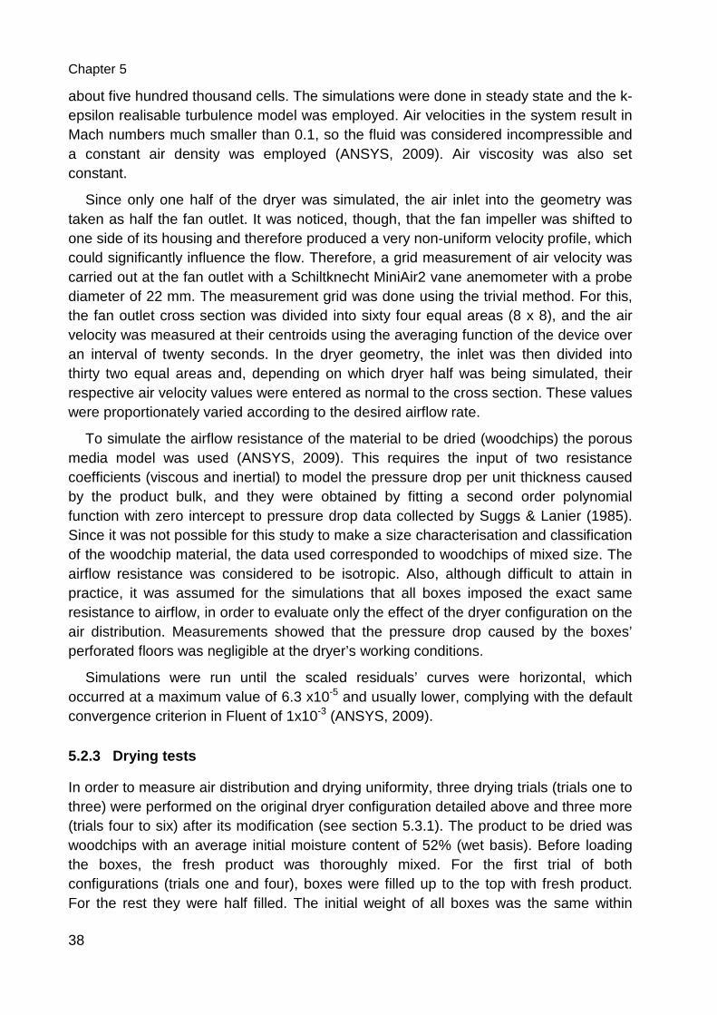
Figure 5.2 Experimental set-up of drying trials ........................................................ 39

Figure 5.3 Pathlines (a) and contours of air velocity (b) for the original dryer configuration ........................................................................................... 40

Figure 5.4 Contours of air velocity at fan outlet (air flow into the sheet) .................. 41

Figure 5.5 Box dryer with wide inlets ....................................................................... 42

Figure 5.6 Contours of air velocity in box dryer with wide inlets .............................. 42

Figure 5.7 Contours of air velocity in diffuser with eight air guides and two perforated plates ..................................................................................... 44

Figure 5.8 Air velocity in the tapered channel in modified dryer configuration: trial 1 left half (a), trial 1 right half (b), trial 2 left half (c), trial 2 right half (d), trial 3 left half (e) and trial 3 right half (f) ................................................. 45

Figure 5.9 Simulation results of airflow through boxes vs. measured average air velocity in the tapered channel, left half of dryer, outer row (a), and right half of dryer, inner row (b) ............................................................... 46

Figure 5.10 Drying curves for the left half of dryer in second trial (a) and the right half in first trial (b) ................................................................................... 48

Figure 5.11 Air velocity in the tapered channel in modified dryer configuration: trial 4 left half (a), trial 4 right half (b), trial 5 left half (c), trial 5 right half (d), trial 6 left half (e) and trial 6 right half (f) ................................................. 49

Figure 5.12 Contours of air velocity at diffusers' outlet, left (a) and right (b) halves of the dryer ............................................................................................. 50

Figure 5.13 Drying curves for the left half of the dryer in fifth trial (a) and the right half in fourth trial (b) ............................................................................... 51

Figure 6.1 Dry matter density profile assumed for perfectly formed bales ............... 56

Figure 6.2 Schematic diagram of basic drying unit .................................................. 59

Figure 6.3 Positions of temperature and air velocity measurements and of samples taken for moisture content determination ................................. 61

Figure 6.4 Air velocity contours and pathlines for the first (a), second (b), third (c) and fourth (d) dryer designs ................................................................... 62

Figure 6.5 Contours of moisture content (a) and temperature (b) for the first design after 7 hours ................................................................................ 63

Figure 6.6 Contours of moisture content (a) and temperature (b) for the second design after 7 hours ................................................................................ 63

Figure 6.7 Contours of moisture content (a) and temperature (b) for the third design after 7 hours ................................................................................ 63

Figure 6.8 Contours of moisture content (a) and temperature (b) for the fourth design after 7 hours ................................................................................ 64

Figure 6.9 Average bale moisture content as function of drying time for the four dryer designs .......................................................................................... 65

Figure 6.10 Percentage of bale volume at different levels of moisture content after 8 hours of drying for the four dryer designs ............................................ 66

Figure 6.11 Dry matter density profile assumed for a bale with irregular density in the axial direction ................................................................................... 67

Figure 6.12 Contours of moisture content after 7 hours for the first (a), second (b), third (c) and fourth (d) dryer designs in bales with non-uniform dry matter density in the axial direction ........................................................ 67

Figure 6.13 Air velocity measured with tapered channel at the bale surface for test 1-1. Each bar in a group refers to a position around bale circumference ......................................................................................... 69

Figure 6.14 Infrared image of test 1-1 after 4 hours of drying .................................... 70

Figure 6.15 Temperature curves in test 1-1 at different bale heights and at a depth of 0.4 m .................................................................................................. 70

Figure 6.16 Air velocity measured with tapered channel at the bale surface for test 2-1. Each bar in a group refers to a position around bale circumference ......................................................................................... 71

Figure 6.17 Temperature curves in test 2-1 at different bale heights and at a depth of 0.4 m ................................................................................................... 71

Figure 6.18 Air velocity measured with tapered channel at the bale surface for tests 3-2 (a) and 3-4 (b). Each bar in a group refers to a position around bale circumference ..................................................................... 72

Figure 6.19 Infrared image for test 3-2 after 3 hours of drying (a) and test 3-4 after 5 hours of drying (b) ............................................................................... 73

Figure 6.20 Temperature curves in test 3-4 at different bale heights and at a depth of 0.4 m ................................................................................................... 73

Figure 6.21 Moisture content after drying at different heights and depths for tests 1-1 (a), 1-3 (b), 2-1 (c), 2-2 (d), 3-3 (e) and 3-4 (f) .................................. 74

Figure 6.22 Comparison of simulation and measured moisture content profiles after drying , at different bale heights and at a bale depth of 0.2 m for test 1-1 (a), 2-1 (b) and 3-4 (f) ................................................................ 75

Figure 7.1 Schematic diagram of test apparatus: inlet duct (a), flow straightener (b), butterfly valve (c), in-line duct fan (d), perforated plates (e), test column (f), outlet duct (g) ........................................................................ 79

Figure 7.2 Measurement positions for the grid measurement .................................. 79

Figure 7.3 Flowchart of the algorithm to calculate the water removed during drying ...................................................................................................... 81

Figure 7.4 Relative (a) and absolute errors (b) in the calculation of the mass of water evaporated in single runs .............................................................. 83

Figure 7.5 Errors in humidity ratio caused by a 0.1 °C error in dry or wet-bulb temperature ............................................................................................ 84

Figure 7.6 Difference in air humidity calculation between inlet and outlet with empty apparatus ..................................................................................... 86

Figure 7.7 Temperature (a) and inlet humidity ratio (b) course of two consecutive runs, the first at nearly constant temperature and the second at varying temperature ................................................................................ 87

Figure 7.8 Real and calculated drying progress for three batches of woodchips (a), (b) and (c), and one batch of fresh alfalfa (d). .................................. 88

Nomenclature

Symbols

a, b, c, d, e, f, k, n model parameters

C* chroma

dh perforate plate hole diameter

ERH equilibrium relative humidity

h hue angle

hs heat of sorption

L* lightness

MR moisture ratio

P pressure

Reh Reynolds number based on the conditions on the holes of the perforated plates

RH relative humidity

s perforated plate thickness

Sh energy source term

Sw moisture source term

T temperature

t time

v air velocity

vh air velocity in the holes of the perforated plates

W moisture content

We equilibrium moisture content

Wo initial moisture content

ζ flow resistance coefficient

ρ air density

ρbd bulk dry matter density of product

φ perforated plate porosity

Acronyms

1D, 2D, 3D One-dimensional, two-dimensional, three-dimensional, respectively

ASABE American Society of Agricultural and Biological Engineers

ASHRAE American Society of Heating, Refrigerating and Air-Conditioning Engineers

CFD Computational fluid dynamics

DAQ Data acquisition device

DLG Deutsche Landwirtschafts-Gesellschaft

FS Full scale

MRE Mean relative error

PVC Polyvinyl chloride

SEE Standard error of the estimate

UDF User-defined function

UDM User-defined memory

UDS User-defined scalar

VDI/VDE Verein Deutscher Ingenieure/Verband der Elektrotechnik Elektronik Informationstechnik

13

1 General introduction

The present work was carried out in the framework of a research project entitled “Experimental investigation and demonstration of sorption energy storage facilities for the low-temperature solar drying” carried out by the Department of Agricultural Engineering and the Department of Solar and Systems Engineering of the University of Kassel. The main objective of the project was to develop and test a liquid desiccant solar energy storage system, and to apply it in the drying of agricultural products. The development of the storage system was carried out by the Department of Solar and Systems Engineering whereas from the Agricultural Engineering point of view the emphasis was in drying tests at low temperatures and the improvement of dryers for medicinal and aromatic plants, and for hay round bales.

Drying is one of the most important methods for the conservation of agricultural products such as grains, herbs and animal feed, and it is at the same time a very energy intensive process. It involves the simultaneous transfer of heat and mass between the product being dried and its surroundings. Although many methods of drying exist, about 85% of industrial dryers are of the convective type where hot air (with or without combustion gases) acts as the drying medium (Arun Mujumdar, 2006) which provides the energy required and carries away the moisture removed. In such systems, as well as in conventional solar dryers, air temperature is increased while its humidity ratio remains constant. On the other hand, in a liquid desiccant system, cold, moist air, such as ambient or recirculated air, is brought in contact with a concentrated hygroscopic salt solution. In this process the air is dehumidified, and the latent heat of vaporization released serves to increase its temperature. The drying air so obtained has a moderate temperature some degrees above the inlet conditions, while having a lower humidity ratio than that which the same inlet air would have if it were heated to the same final temperature. For products requiring low process temperatures, such as medicinal and aromatic plants, hay and others, this air could result in increased drying rates and improved quality. To complete the process cycle, the diluted salt solution must be concentrated back, which can be done at relatively low temperatures achievable with non-concentrating solar thermal systems.

Several factors affect the drying rate of a product and the performance of convective dryers. Each agricultural product is unique in its drying behaviour but also pre-treatments or operations previous to the drying process to which a product is subjected have an effect on drying. In the case of medicinal plants or hay, for instance, they may be dried as entire plants (stems and leaves), they may be previously cut to different sizes, or even a separation of leaves and stems may be attempted, since these two plant parts also dry at different rates.

A purely theoretical description of the drying process in an actual dryer requires knowledge of the mechanisms of drying in a single product particle or a single, thin layer. Although different theories and theoretical models have been proposed to

General introduction

14

describe the drying behaviour of agricultural products as individual particles, only semi-theoretical and theoretical relationships have proved useful so far (Brooker et al., 1992). Thus, experimental studies on thin-layer drying have been and are still being performed for many crops under various external (air) conditions and product pre-treatments. Then, a number of empirical models can be fitted to the data and the best selected to be able to estimate the drying curve of the product within the range of conditions studied. All of these studies attribute the greatest effect on drying rate to air temperature. In many cases the effect of air velocity on thin-layer drying has not been studied or was found negligible, whereas in other cases the drying rate in fact increased when air velocity increased up to a given value, and especially at high moisture contents (Kashaninejad et al., 2007; Khatchatourian, 2012; Sturm, 2010). Similarly, and most importantly for this study, although some studies indicate an appreciable effect of air humidity (Ajibola, 1989; Argyropoulos & Müller, 2011; Corrêa et al., 1999), in many cases air humidity was not studied (Belghit et al., 2000; Doymaz, 2011; Wang et al., 2007) or its effect was considered to be insignificant (Arabhosseini et al., 2009; Dandamrongrak et al., 2002; Madamba et al., 1996; Panchariya et al., 2002). However, in most of these last cases the levels of relative humidity considered were in a very narrow range and/or very low, which might not be enough to discern an effect.

In many practical dryers crops are not dried in a single, thin layer but as a bulk with depths varying from below one to several meters. In them, even if the conditions of the drying air at the inlet are maintained constant, as the air flows from inlet to outlet they change continuously (i.e. from warm, dry air to cool, moist air) so that the drying rate varies not only as a function of time but also as a function of position in the bulk. Thus, thin-layer drying equations by themselves are of little use for the prediction of the drying behaviour in bulks. However, comprehensive mathematical models for the simulation of deep bed drying usually make use of such equations. In them the bulk is divided into a considerable number of thin layers. A set of partial differential equations must be solved which represent the energy and mass balance in each layer. Since the resulting system of equations with initial and boundary conditions cannot be solved analytically numerical techniques are required. Additionally, psychrometric relationships to calculate relevant air properties and a moisture isotherm equation must be available (Brooker et al., 1992).

In general when deep bed drying simulations are performed, some assumptions are made in order to simplify the problem, such as a negligible shrinkage, negligible heat conduction from particle to particle, constant air and product properties and very importantly, the existence of plug flow of air. This last assumption means that the drying air flows at a constant velocity from inlet to outlet in straight, parallel lines, and thus the problem can be reduced to one dimension. Although this can be valid in a number of situations, the flow in many dryers is not so simple. In reality there might be significant variation in air velocity (magnitude and direction) at different positions in the dryer. The drying rate is a strong function of airflow and air velocity, and therefore, it is of great importance to know the airflow and velocity in the drying chamber, which allows knowing the areas of adequate air velocities for proper drying (Xia & Sun, 2002). The

General introduction

15

dryer design itself is an important cause for the non-uniform air distribution encountered in practice. In grain dryers, for instance, the use of on-floor ducts in the bin produces non-linear flow (Brooker et al., 1992). Also, if during filling of the bin the grain mass forms a peaked cone as opposed to a levelled surface, the air velocity will be higher close to the walls than at the middle (Lawrence & Maier, 2012). Another cause for deficient air distribution is the variation in bulk density at different locations in the product bulk, since this will determine the resistance to air flow. This is particularly important in the drying of herbs and hay, since a bed of these products can vary significantly in bulk density depending on the filling method, bulk height and whether some regions in the bed received more compression than others. Thus, in cases where plug flow cannot be assumed, the problem is no longer one dimensional, and the drying of a product bulk depends on the flow field through it in a more complex manner.

The branch of computational fluid dynamics (CFD) uses computers and applied mathematics to model fluid flow situations (Xia & Sun, 2002). Recent progression in computing efficacy coupled with reduced costs of CFD software packages has advanced it as a viable technique to provide effective and efficient design solutions (Norton & Sun, 2006). The steps required to complete a CFD simulation are separated into the pre-processing, processing, and post-processing. Pre-processing includes all the tasks required before the actual solution process begins and comprises the geometry definition; the meshing, which refers to the subdivision of the geometry into numerous elements or cells so that the discretized governing equations are solved in each of them; and the set-up of the solver and the selection of appropriate models. Processing is the main part and refers to the iterative solution of the governing equations with the boundary and initial conditions specified by the user. Finally the post-processing part refers to the data analysis and visualization. One of the first studies which applied CFD on drying was done by Mathioulakis et al. (1998), in which the air distribution in a tray dryer was simulated. Afterwards a number of other studies has followed, most of them also using CFD to simulate air distribution in different types of dryers (Amanlou & Zomorodian, 2010; Margaris & Ghiaus, 2006; Mirade & Daudin, 2000; Mirade, 2003). Such flow simulations allow the air distribution in the dryer to be visualized, facilitating the identification of possibilities for design changes. Then, the performance of modified designs can also be simulated without the need to physically construct the model and test it. However, simulation results should still be validated by experiments because CFD uses many approximate models as well as a few assumptions (Xia & Sun, 2002). Additionally, CFD packages usually allow customization to enhance their capabilities. In this way, the drying process can also be simulated by introducing the necessary variables, scalar quantities and equations. In this case the drying progress throughout the product bulk will depend on the flow field. Thus, for example, if part of the bulk is modelled as being strongly compressed in comparison with other regions, the simulation results will show a decreased airflow through it and consequently a slower drying rate.

General introduction

16

The monitoring of the drying process is in most cases complicated since the moisture content of the product usually varies from location to location in the dryer, and determining an average value might require the extraction of several or many samples, whose moisture cannot, in many cases, be determined immediately. In convective batch dryers the use of psychrometric and airflow measurements could offer a relatively simple method to estimate the average moisture of the batch continuously. Although some studies have used this method to estimate the drying progress, no comparison was made to measurements in order to determine its accuracy.

17

2 Objectives of the research

The objectives of this research were related to the research project from which it stemmed. Since in conventional convective drying systems ambient air is simply heated up while its humidity ratio remains constant and in the sorption system both an increase in temperature and a dehumidification take place, a first objective was, given the lack of studies, to find out if the effect of air humidity in the drying rate of agricultural products such as herbs and hay is negligible at the low temperatures which are to be supplied by the liquid desiccant system, as it seems to be at higher temperatures. This was done using a particular aromatic plant, leaf celery, as an example product with a relatively important production in Germany and for which no information about its drying behaviour is yet available. Also to this aim, sorption isotherm relationships for this product were determined experimentally.

Due to the importance of an optimal air distribution on the performance of convective dryers, it was also aimed in this work to study, by means of experimental measurements and by the use of computational fluid dynamics software, the air flow characteristics of conventional dryers used for herbs and spices, which are typically dried in loose form, and for round hay bales, which are good examples of compressed bulks with variable dry matter density. It was further aimed, following the results and using these same methods, to test different possibilities for improvement leading to more efficient dryers.

Finally, it was aimed to study the accuracy of airflow and psychrometric measurements to calculate water evaporation from the product in convective batch-type dryers, which would provide a simple method useful in monitoring the average moisture content and thus estimate the end of the process.

18

3 Sorption Isotherms of Celery Leaves ( Apium graveolens var. secalinum)

Sorption isotherms provide important information for the drying process and storage of foodstuffs. The desorption isotherms of celery leaves at three temperatures (25, 40 and 50 °C) as well as their adsorption isotherm at 25 °C were experimentally determined by means of the static gravimetric method, using eight saturated salt solutions with relative humidities in the range from 11 to 84%. Six mathematical models (Halsey, Oswin, Henderson, GAB, Peleg and BET) were fitted to the data. The Peleg model resulted in the lowest error in all cases. A modification of the Peleg model was attempted to incorporate the effect of temperature in the desorption process. The fitting was satisfactory, providing a single equation for calculation of the equilibrium conditions within the studied temperature range.

3.1 Introduction

Celery (Apium graveolens L.) is a plant species of the family Apiaceae. Leaf celery (Apium graveolens L. var. secalinum), also known as cutting celery, is a variety in which the usable parts are the dark-green, glossy leaves on long, thin leaf petioles, presenting a strong celery flavor. They may be eaten fresh or processed, mainly frozen or dried (Rożek, 2007). Although not as well known as celeriac (Apium graveolens L. var. rapaceum), it is an economically important herb in Germany, with 136 ha of cultivated area in 2003 (Hoppe, 2005).

In general leaves require less time and energy for drying than other parts of plants, which makes celery leaves more suitable for the drying process compared to the stalk or root parts commonly used in the other varieties.

Sorption isotherms define the hygroscopic equilibrium between the relative humidity and moisture content at a given temperature. Thus, they provide important information for the drying process and storage of foods and other products.

3.2 Materials and methods

3.2.1 Plant material

Leaf celery (Apium graveolens var. secalinum) was sowed in pots in mid March and kept in a greenhouse until late May, when the plants were moved into the research field of the Agricultural Engineering Department of Kassel University in Witzenhausen in the year 2009. Plants were harvested manually and leaves separated immediately before each trial.

Chapter 3

19

3.2.2 Experimental procedure

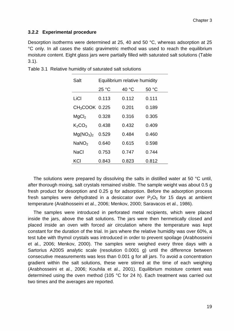
Desorption isotherms were determined at 25, 40 and 50 °C, whereas adsorption at 25 °C only. In all cases the static gravimetric method was used to reach the equilibrium moisture content. Eight glass jars were partially filled with saturated salt solutions (Table 3.1).

Table 3.1 Relative humidity of saturated salt solutions

Salt Equilibrium relative humidity

25 °C 40 °C 50 °C

LiCl 0.113 0.112 0.111

CH3COOK 0.225 0.201 0.189

MgCl2 0.328 0.316 0.305

K2CO3 0.438 0.432 0.409

Mg(NO3)2 0.529 0.484 0.460

NaNO2 0.640 0.615 0.598

NaCl 0.753 0.747 0.744

KCl 0.843 0.823 0.812

The solutions were prepared by dissolving the salts in distilled water at 50 °C until, after thorough mixing, salt crystals remained visible. The sample weight was about 0.5 g fresh product for desorption and 0.25 g for adsorption. Before the adsorption process fresh samples were dehydrated in a desiccator over P2O5 for 15 days at ambient temperature (Arabhosseini et al., 2006; Menkov, 2000; Saravacos et al., 1986).

The samples were introduced in perforated metal recipients, which were placed inside the jars, above the salt solutions. The jars were then hermetically closed and placed inside an oven with forced air circulation where the temperature was kept constant for the duration of the trial. In jars where the relative humidity was over 60%, a test tube with thymol crystals was introduced in order to prevent spoilage (Arabhosseini et al., 2006; Menkov, 2000). The samples were weighed every three days with a Sartorius A200S analytic scale (resolution 0.0001 g) until the difference between consecutive measurements was less than 0.001 g for all jars. To avoid a concentration gradient within the salt solutions, these were stirred at the time of each weighing (Arabhosseini et al., 2006; Kouhila et al., 2001). Equilibrium moisture content was determined using the oven method (105 °C for 24 h). Each treatment was carried out two times and the averages are reported.

Chapter 3

20

3.2.3 Model fitting

From the many mathematical models found in the literature to describe sorption isotherms, six were selected and fitted to each temperature’s results (Table 3.2). The statistics software SPSS 17 was used to fit the models to the data using the nonlinear regression function. To be sure that the parameters obtained were the optimal, each regression was repeated with different starting parameter values.

Table 3.2 Sorptions isotherms models fitted to the experimental data

Model Equation Source

Halsey �� = � −�ln(�� )��� 3.1

(Iglesias & Chirife, 1982)

Oswin �� = � � �� 1 − �� �� 3.2

(Iglesias & Chirife, 1982; Park et al., 2002)

Henderson �� = �−��(1 − �� )� ��� 3.3

(da Silva et al., 2004; Iglesias & Chirife, 1982)

GAB �� = ����� (1 − ��� )(1 − ��� + ���� ) 3.4 (ASABE, 2008)

Peleg �� = ��� � + ��� � 3.5 (Peleg, 1993)

BET �� = ���� (1 − �� )�1 + �� (� − 1)� 3.6 (Liendo-Cárdenas et al., 2000)

where We is the equilibrium moisture content d.b.; ERH the equilibrium relative humidity; and a, b, c, d the models’ parameters.

The goodness of fit of the equations was evaluated using the coefficient of determination R2 together with the mean relative error, MRE, and the standard error of the estimate, SEE (Mehta & Singh, 2006; Soysal & Öztekin, 1999; Sun, 1999):

��� = 1� � �� − �!� ��"

#$� 3.7

Chapter 3

21

%�� = &� ��� − �!��� − ' ("#$� 3.8

where n is the number of experimental points, and p the number of parameters.

Additionally, residuals were plotted against relative humidity and visually assessed for randomness (Menkov, 2000; Soysal & Öztekin, 1999).

3.3 Results and discussion

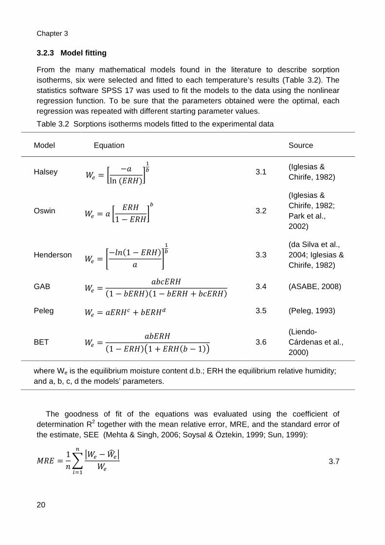
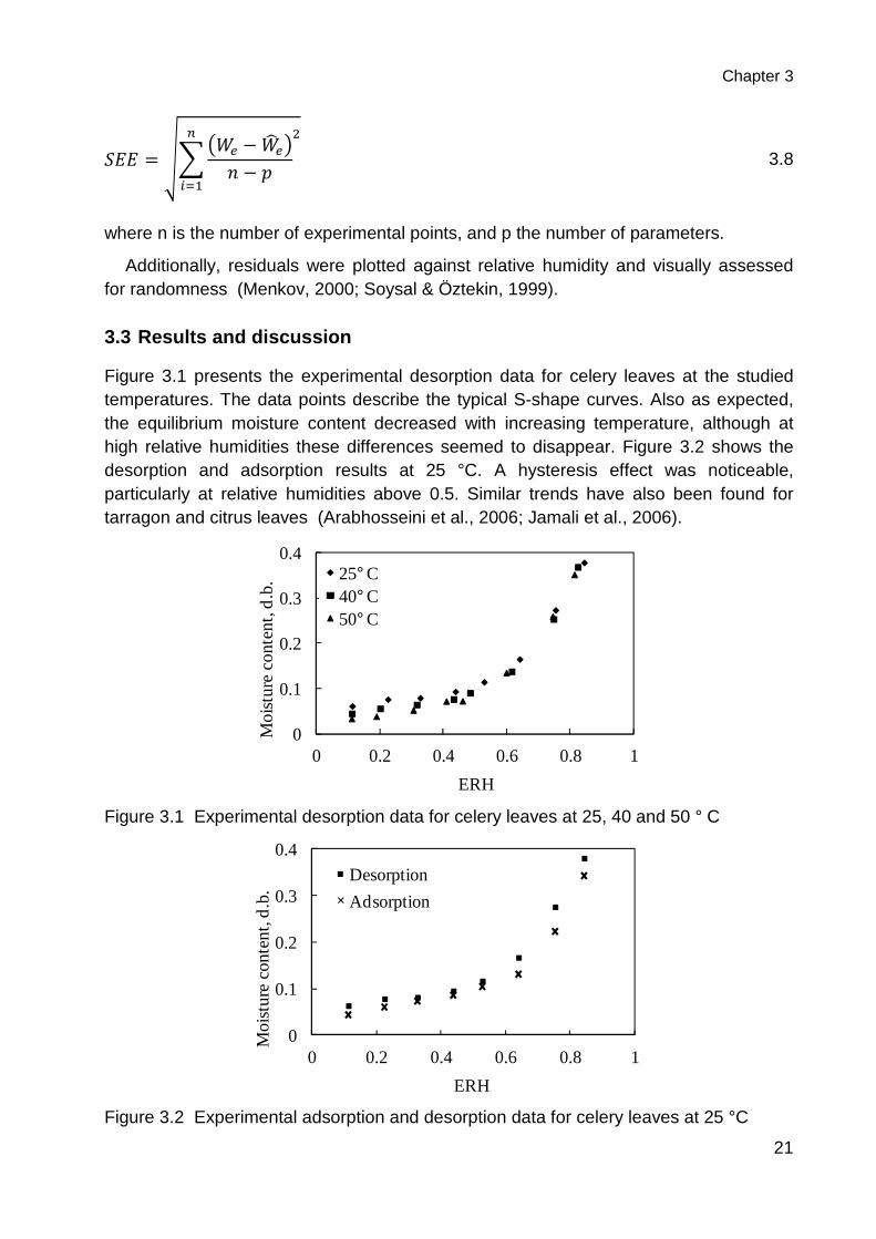
Figure 3.1 presents the experimental desorption data for celery leaves at the studied temperatures. The data points describe the typical S-shape curves. Also as expected, the equilibrium moisture content decreased with increasing temperature, although at high relative humidities these differences seemed to disappear. Figure 3.2 shows the desorption and adsorption results at 25 °C. A hysteresis effect was noticeable, particularly at relative humidities above 0.5. Similar trends have also been found for tarragon and citrus leaves (Arabhosseini et al., 2006; Jamali et al., 2006).

Figure 3.1 Experimental desorption data for celery leaves at 25, 40 and 50 ° C

Figure 3.2 Experimental adsorption and desorption data for celery leaves at 25 °C

0

0.1

0.2

0.3

0.4

0 0.2 0.4 0.6 0.8 1

Mo

istu

re c

ont

ent,

d.b

.

ERH

25° C40° C50° C

0

0.1

0.2

0.3

0.4

0 0.2 0.4 0.6 0.8 1

Moi

stu

re c

onte

nt,

d.b

.

ERH

Desorption

Adsorption

Chapter 3

22

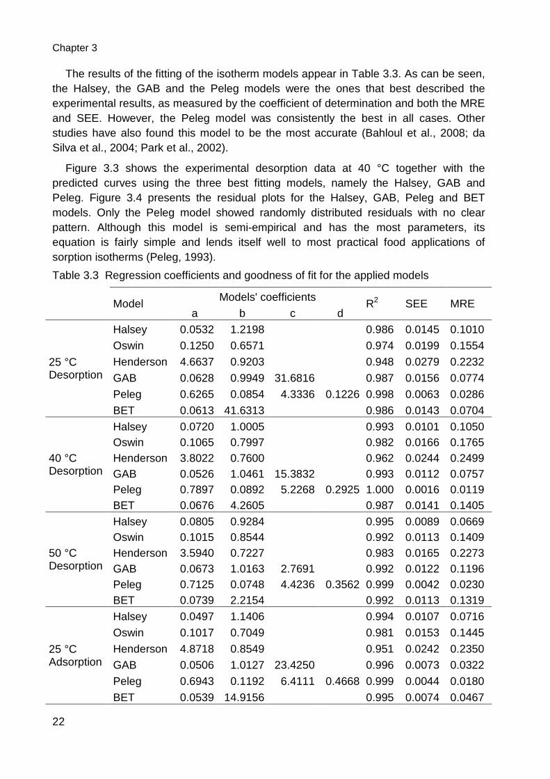
The results of the fitting of the isotherm models appear in Table 3.3. As can be seen, the Halsey, the GAB and the Peleg models were the ones that best described the experimental results, as measured by the coefficient of determination and both the MRE and SEE. However, the Peleg model was consistently the best in all cases. Other studies have also found this model to be the most accurate (Bahloul et al., 2008; da Silva et al., 2004; Park et al., 2002).

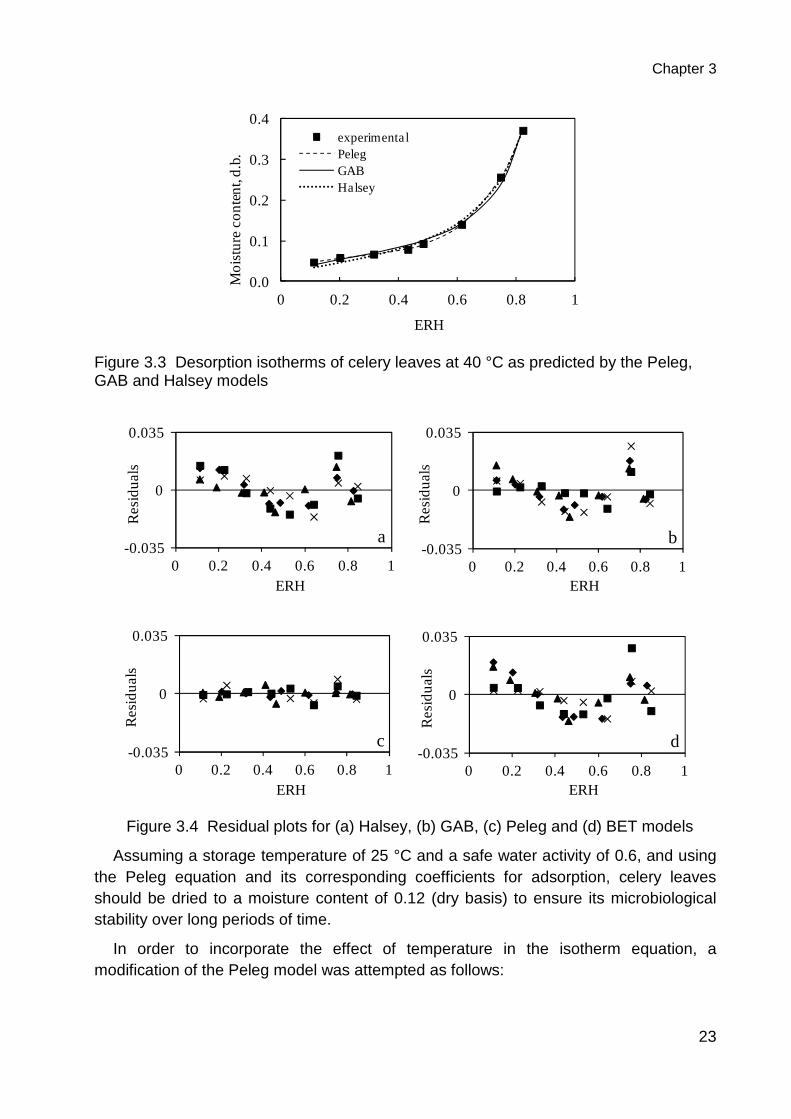
Figure 3.3 shows the experimental desorption data at 40 °C together with the predicted curves using the three best fitting models, namely the Halsey, GAB and Peleg. Figure 3.4 presents the residual plots for the Halsey, GAB, Peleg and BET models. Only the Peleg model showed randomly distributed residuals with no clear pattern. Although this model is semi-empirical and has the most parameters, its equation is fairly simple and lends itself well to most practical food applications of sorption isotherms (Peleg, 1993).

Table 3.3 Regression coefficients and goodness of fit for the applied models

Model

Models' coefficients R2 SEE MRE

a b c d

25 °C Desorption

Halsey 0.0532 1.2198 0.986 0.0145 0.1010

Oswin 0.1250 0.6571 0.974 0.0199 0.1554

Henderson 4.6637 0.9203 0.948 0.0279 0.2232

GAB 0.0628 0.9949 31.6816 0.987 0.0156 0.0774

Peleg 0.6265 0.0854 4.3336 0.1226 0.998 0.0063 0.0286

BET 0.0613 41.6313 0.986 0.0143 0.0704

40 °C Desorption

Halsey 0.0720 1.0005 0.993 0.0101 0.1050 Oswin 0.1065 0.7997 0.982 0.0166 0.1765 Henderson 3.8022 0.7600 0.962 0.0244 0.2499 GAB 0.0526 1.0461 15.3832 0.993 0.0112 0.0757 Peleg 0.7897 0.0892 5.2268 0.2925 1.000 0.0016 0.0119 BET 0.0676 4.2605 0.987 0.0141 0.1405

50 °C Desorption

Halsey 0.0805 0.9284 0.995 0.0089 0.0669 Oswin 0.1015 0.8544 0.992 0.0113 0.1409 Henderson 3.5940 0.7227 0.983 0.0165 0.2273 GAB 0.0673 1.0163 2.7691 0.992 0.0122 0.1196 Peleg 0.7125 0.0748 4.4236 0.3562 0.999 0.0042 0.0230 BET 0.0739 2.2154 0.992 0.0113 0.1319

25 °C Adsorption

Halsey 0.0497 1.1406 0.994 0.0107 0.0716

Oswin 0.1017 0.7049 0.981 0.0153 0.1445

Henderson 4.8718 0.8549 0.951 0.0242 0.2350

GAB 0.0506 1.0127 23.4250 0.996 0.0073 0.0322

Peleg 0.6943 0.1192 6.4111 0.4668 0.999 0.0044 0.0180

BET 0.0539 14.9156 0.995 0.0074 0.0467

Chapter 3

23

Figure 3.3 Desorption isotherms of celery leaves at 40 °C as predicted by the Peleg, GAB and Halsey models

Figure 3.4 Residual plots for (a) Halsey, (b) GAB, (c) Peleg and (d) BET models

Assuming a storage temperature of 25 °C and a safe water activity of 0.6, and using the Peleg equation and its corresponding coefficients for adsorption, celery leaves should be dried to a moisture content of 0.12 (dry basis) to ensure its microbiological stability over long periods of time.

In order to incorporate the effect of temperature in the isotherm equation, a modification of the Peleg model was attempted as follows:

0.0

0.1

0.2

0.3

0.4

0 0.2 0.4 0.6 0.8 1

Mo

istu

re c

on

ten

t, d

.b.

ERH

experimentalPelegGABHalsey

-0.035

0

0.035

0 0.2 0.4 0.6 0.8 1

Re

sid

ua

ls

ERH

a-0.035

0

0.035

0 0.2 0.4 0.6 0.8 1

Re

sid

ua

ls

ERH

b

-0.035

0

0.035

0 0.2 0.4 0.6 0.8 1

Re

sid

ua

ls

ERH

c-0.035

0

0.035

0 0.2 0.4 0.6 0.8 1

Re

sid

ua

ls

ERH

d

Chapter 3

24

Modified Peleg �� = (� + �))�� � + (* + +))�� , 3.9

where T is the temperature in °C. The calculated regression parameters were in this case 0.5006, 0.0052, 4.5595, 0.1299, -0.0013 and 0.2102 respectively. The coefficient of determination R2, the MRE and the SEE were 0.998, 0.0390 and 0.0052 respectively, resulting in a very good fit, whose predicted curves at the studied temperatures resemble closely those predicted individually by the original model. Thus, this modified model can be used as a single equation to estimate the equilibrium conditions of celery leaves in the studied temperature range.

3.4 Conclusions

The sorption isotherms of celery leaves followed the usual trends of shape and temperature dependence. For their storage at 25 °C or less, a maximum moisture content of 0.12 (dry basis) must be reached. From the six models tested, the Peleg model with four parameters offered the smallest error in all cases. A modified version of this model to include the effect of temperature fitted well to all the desorption data, resulting in an equation with six parameters, from which the equilibrium conditions at any temperature from 25 to 50 °C can be estimated. These results will serve to model the thin-layer drying behavior of celery leaves at various air temperatures and relative humidities.

25

4 Effect of air temperature and relative humidity on the thin-layer drying of celery leaves ( Apium graveolens var. secalinum)

The thin-layer drying of celery leaves was studied under different conditions of air temperature (20-50 °C) and relative humidity (10-60%) in a through-flow laboratory dryer. Both parameters influenced the drying time, although the effect of air temperature was more pronounced. The effect of air relative humidity was practically negligible at 50 °C. The experimental data was fitted to six thin-layer drying models and their goodness of fit was tested, being the Two-term exponential model the one that showed the best fit in the majority of treatments. The relationship between drying conditions and regression parameters of this model was analyzed to include it in the model. Parameter a had a negligible effect on the drying curves and was set constant. For parameter k a piecewise function was used in two parts, one for the temperatures between 20 and 40 °C and the other for 40 to 50 °C, resulting in a good fit overall. The color of the dried leaves did not appreciably change at temperatures between 20 and 40 °C, except at very high levels of relative humidity, which should be avoided when air recirculation is used. At 50 °C color was negatively affected.

4.1 Introduction

Celery (Apium graveolens L.) is a plant species of the family Apiaceae. It is one of the oldest cultivated plants to be used for medicinal and dietary purposes. Today is mostly used as food and condiment (Mielke & Schöber-Butin, 2007). Leaf celery (Apium graveolens L. var. secalinum), also known as cutting celery, is a variety in which the usable parts are the dark-green, glossy leaves on long, thin leaf petioles, presenting a strong celery flavor. They may be eaten fresh or processed, mainly frozen or dried, with which their aroma is not lost (Mielke & Schöber-Butin, 2007; Rożek, 2007). Although not as well known as celeriac (Apium graveolens L. var. rapaceum), it is an economically important herb in Germany, with 136 ha of cultivated area in 2003 (Hoppe, 2005).

In general leaves require less time and energy for drying than other parts of plants, which makes celery leaves more suitable for the drying process compared to the stalk or root parts commonly used in the other varieties.

The thin-layer drying behaviour of many medicinal plants and spices has been studied. No literature was however found for celery leaves. Moreover, the majority of studies have considered only temperature as a drying parameter. Only a few have studied the effect of air relative humidity, mostly within small ranges and at relatively high temperatures, finding in most cases a negligible effect of this parameter (Hosseini, 2005; Madamba et al., 1996; Phupaichitkun, 2008).

The objective of this study was to determine the effect of air temperature and relative humidity on the thin-layer drying of celery leaves; find a best mathematical model which includes these effects; and determine the difference in color between treatments.

Chapter 4

26

4.2 Materials and Methods

4.2.1 Plant Material

Leaf celery (Apium graveolens var. secalinum) was sowed in pots in mid March and kept in a greenhouse until late May, when the plants were moved into the research field of the Agricultural Engineering Department of Kassel University in Witzenhausen in the year 2009. Plants were harvested manually and leaves separated immediately before each trial.

4.2.2 Drying apparatus

The laboratory dryer consisted of a drying chamber, an axial fan and an air preconditioning chamber. The drying chamber contained two trays whose bottoms where made of metal mesh to allow air to flow vertically through the product. Each tray had dimensions 0.25 m x 0.16 m and rested over air channels with two perforated plates placed in series to improve the air distribution. Air flow delivered by the fan was controlled using a laboratory power supply and an Airflow TA-5 hot-wire anemometer. The heating system in the preconditioning chamber allowed the air temperature to be fixed at the desired level, whereas the air relative humidity was increased when needed using an air humidifier. The humidity was controlled using a relative humidity regulator and measured with an Ahlborn Therm 2286-2 electronic psychrometer.

4.2.3 Experimental Procedure

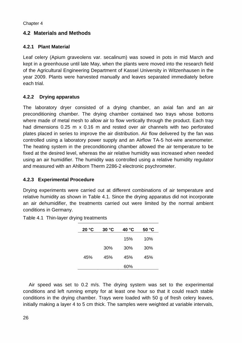
Drying experiments were carried out at different combinations of air temperature and relative humidity as shown in Table 4.1. Since the drying apparatus did not incorporate an air dehumidifier, the treatments carried out were limited by the normal ambient conditions in Germany.

Table 4.1 Thin-layer drying treatments

20 °C 30 °C 40 °C 50 °C

15% 10%

30% 30% 30%

45% 45% 45% 45%

60%

Air speed was set to 0.2 m/s. The drying system was set to the experimental conditions and left running empty for at least one hour so that it could reach stable conditions in the drying chamber. Trays were loaded with 50 g of fresh celery leaves, initially making a layer 4 to 5 cm thick. The samples were weighted at variable intervals,

Chapter 4

27

more often at the beginning and at the end of the trials than in the middle, and depending on the drying temperature. The weighing was done in a Sartorius E2000D electronic scale with a resolution of 0.01 g. The trials were stopped when the sample mass did not change anymore. The dry weight of the samples was determined using the oven method (105 °C for 24 h), from which the moisture content at every weighing time was derived. Two replications were carried out for each treatment.

At the end of each trial the color of a sample of ten leaves was measured with a colorimeter Konica Minolta CR-400, using the L*C*h color space, where L* is the lightness from 0 (black) to 100 (white); h is the hue angle, where 0° corresponds to the positive a-axis of the CIELAB color space (red), 90° to the positive b-axis (yellow), 180° to the negative a-axis (green) and 270° to the negative b-axis (blue); and C* is the chroma or saturation from 0 to 60.

4.2.4 Model fitting

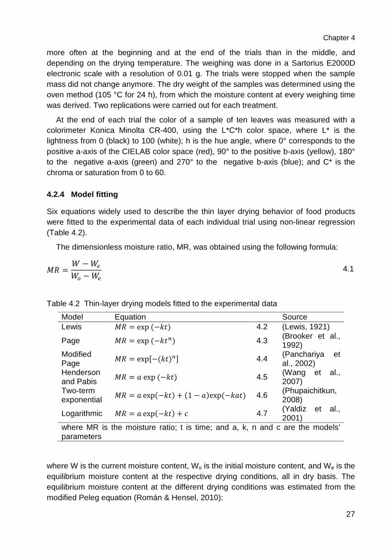
Six equations widely used to describe the thin layer drying behavior of food products were fitted to the experimental data of each individual trial using non-linear regression (Table 4.2).

The dimensionless moisture ratio, MR, was obtained using the following formula:

�� = � − ���- − �� 4.1

Table 4.2 Thin-layer drying models fitted to the experimental data

Model Equation Source Lewis �� = exp(−12) 4.2 (Lewis, 1921)

Page �� = exp(−12") 4.3 (Brooker et al., 1992)

Modified Page �� = exp3−(12)"4 4.4

(Panchariya et al., 2002)

Henderson and Pabis �� = �exp(−12) 4.5

(Wang et al., 2007)

Two-term exponential �� = � exp(−12) + (1 − �)exp(−1�2) 4.6

(Phupaichitkun, 2008)

Logarithmic �� = � exp(−12) + � 4.7 (Yaldiz et al., 2001)

where MR is the moisture ratio; t is time; and a, k, n and c are the models’ parameters

where W is the current moisture content, Wo is the initial moisture content, and We is the equilibrium moisture content at the respective drying conditions, all in dry basis. The equilibrium moisture content at the different drying conditions was estimated from the modified Peleg equation (Román & Hensel, 2010):

Chapter 4

28

�� = (0.5006 + 0.0052))�� :.;;<; + (0.1299 − 0.0013))�� ?.(�?( 4.8

For the treatment at 20 °C in this study, the equilibrium moisture content was extrapolated.

The fitting was done using the non-linear regression function of SPSS 18. The coefficient of determination (R2) and the standard error of estimate (SEE) were used to evaluate the goodness of fit of the equations. The equation for the SEE is as follows:

%�� = &� ��� − �!��@ − ' (A#$� 4.9

where m is the number of experimental points and p the number of regression parameters.

The best model was chosen for further analysis, which attempted to include in the model the relationship between the drying variables studied and the regression parameters.

4.3 Results and discussion

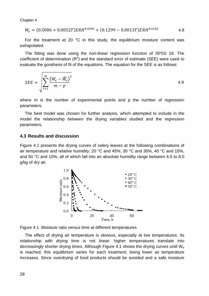
Figure 4.1 presents the drying curves of celery leaves at the following combinations of air temperature and relative humidity: 20 °C and 45%, 30 °C and 30%, 40 °C and 15%, and 50 °C and 10%, all of which fall into an absolute humidity range between 6.5 to 8.0 g/kg of dry air.

Figure 4.1 Moisture ratio versus time at different temperatures

The effect of drying air temperature is obvious, especially at low temperatures. Its relationship with drying time is not linear: higher temperatures translate into decreasingly shorter drying times. Although Figure 4.1 shows the drying curves until We is reached, this equilibrium varies for each treatment, being lower as temperature increases. Since overdrying of food products should be avoided and a safe moisture

0.0

0.2

0.4

0.6

0.8

1.0

0 20 40 60

Mo

istu

re r

atio

Time, h

20° C30° C40° C50° C

Chapter 4

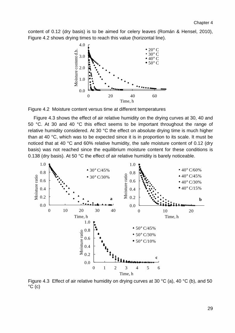
29

content of 0.12 (dry basis) is to be aimed for celery leaves (Román & Hensel, 2010), Figure 4.2 shows drying times to reach this value (horizontal line).

Figure 4.2 Moisture content versus time at different temperatures

Figure 4.3 shows the effect of air relative humidity on the drying curves at 30, 40 and 50 °C. At 30 and 40 °C this effect seems to be important throughout the range of relative humidity considered. At 30 °C the effect on absolute drying time is much higher than at 40 °C, which was to be expected since it is in proportion to its scale. It must be noticed that at 40 °C and 60% relative humidity, the safe moisture content of 0.12 (dry basis) was not reached since the equilibrium moisture content for these conditions is 0.138 (dry basis). At 50 °C the effect of air relative humidity is barely noticeable.

Figure 4.3 Effect of air relative humidity on drying curves at 30 °C (a), 40 °C (b), and 50 °C (c)

0.0

1.0

2.0

3.0

4.0

0 20 40 60

Mo

istu

re c

on

ten

t d.b

.

Time, h

20° C30° C40° C50° C

0.0

0.2

0.4

0.6

0.8

1.0

0 10 20 30 40

Mo

istu

re r

atio

Time, h

30° C/45%

30° C/30%

a

0.0

0.2

0.4

0.6

0.8

1.0

0 10 20

Mo

istu

re r

atio

Time, h

40° C/60%40° C/45%40° C/30%40° C/15%

b

0.0

0.2

0.4

0.6

0.8

1.0

0 1 2 3 4 5 6

Mo

istu

re ra

tio

Time, h

50° C/45%

50° C/30%

50° C/10%

c

Chapter 4

30

Müller (1992) reported an almost linear increase in the drying time of common sage at 50 °C when the air relative humidity increased from 10 to 50%, followed by an exponential increase from 50% onwards. In the same work he reported a very small influence in the drying of chamomile flowers at 60 °C when relative humidity increased from 10 to 40% and from 50% onwards the drying time was more strongly affected. Phupaichitkun (2008) reported a negligible influence of this parameter on drying rate of longan fruits, however the range of humidity studied was only from 4 to 20% and at 80 °C. Hosseini (2005) studied the thin-layer drying behaviour of tarragon and concluded that the relative humidity range applied did not have a significant effect in the drying rate. However his study was done at temperatures from 40 to 90 °C, and the relative humidity level within each temperature was varied in up to 15 percentage points, which could explain their conclusion. Although more information is needed, it could be hypothesized that in general, as air temperature increases, the air relative humidity plays a less important role in the drying of celery leaves and other agricultural products.

4.3.1 Model fitting

The results of the non-linear regression procedure showed that the logarithmic model, although providing a very good fit with the data as determined by both R2 and SEE, resulted for all trials in negative predicted values of MR for the last stage of the drying experiments. This is due to its third parameter, which allows the MR to acquire negative values, unlike the other five equations. Thus, the logarithmic model was not considered for further analysis.

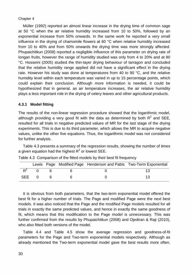
Table 4.3 presents a summary of the regression results, showing the number of times a given equation had the highest R2 or lowest SEE.

Table 4.3 Comparison of the fitted models by their best fit frequency

Lewis Page Modified Page Henderson and Pabis Two-Term Exponential

R2 0 6 6 0 13

SEE 0 6 6 0 13

It is obvious from both parameters, that the two-term exponential model offered the best fit for a higher number of trials. The Page and modified Page were the next best models. It was also noticed that the Page and the modified Page models resulted for all trials in exactly the same predicted values, and hence in exactly the same goodness of fit, which means that this modification to the Page model is unnecessary. This was further confirmed from the results by Phupaichitkun (2008) and Ojediran & Raji (2010), who also fitted both versions of the model.

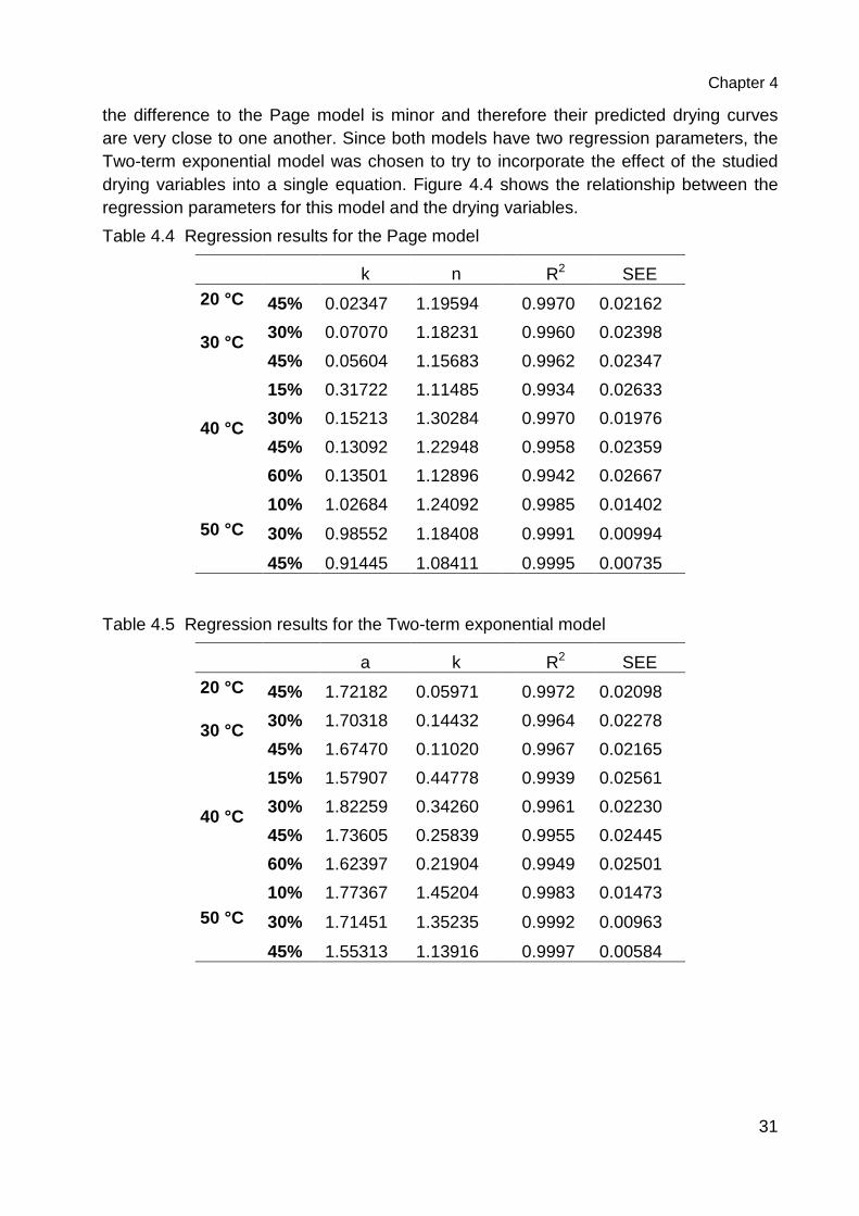
Table 4.4 and Table 4.5 show the average regression and goodness-of-fit parameters for the Page and Two-term exponential models respectively. Although as already mentioned the Two-term exponential model gave the best results more often,

Chapter 4

31

the difference to the Page model is minor and therefore their predicted drying curves are very close to one another. Since both models have two regression parameters, the Two-term exponential model was chosen to try to incorporate the effect of the studied drying variables into a single equation. Figure 4.4 shows the relationship between the regression parameters for this model and the drying variables.

Table 4.4 Regression results for the Page model

k n R2 SEE 20 °C 45% 0.02347 1.19594 0.9970 0.02162

30 °C 30% 0.07070 1.18231 0.9960 0.02398

45% 0.05604 1.15683 0.9962 0.02347

40 °C

15% 0.31722 1.11485 0.9934 0.02633

30% 0.15213 1.30284 0.9970 0.01976

45% 0.13092 1.22948 0.9958 0.02359

60% 0.13501 1.12896 0.9942 0.02667

50 °C 10% 1.02684 1.24092 0.9985 0.01402

30% 0.98552 1.18408 0.9991 0.00994

45% 0.91445 1.08411 0.9995 0.00735

Table 4.5 Regression results for the Two-term exponential model

a k R2 SEE 20 °C 45% 1.72182 0.05971 0.9972 0.02098

30 °C 30% 1.70318 0.14432 0.9964 0.02278

45% 1.67470 0.11020 0.9967 0.02165

40 °C

15% 1.57907 0.44778 0.9939 0.02561

30% 1.82259 0.34260 0.9961 0.02230

45% 1.73605 0.25839 0.9955 0.02445

60% 1.62397 0.21904 0.9949 0.02501

50 °C 10% 1.77367 1.45204 0.9983 0.01473

30% 1.71451 1.35235 0.9992 0.00963

45% 1.55313 1.13916 0.9997 0.00584

Chapter 4

32

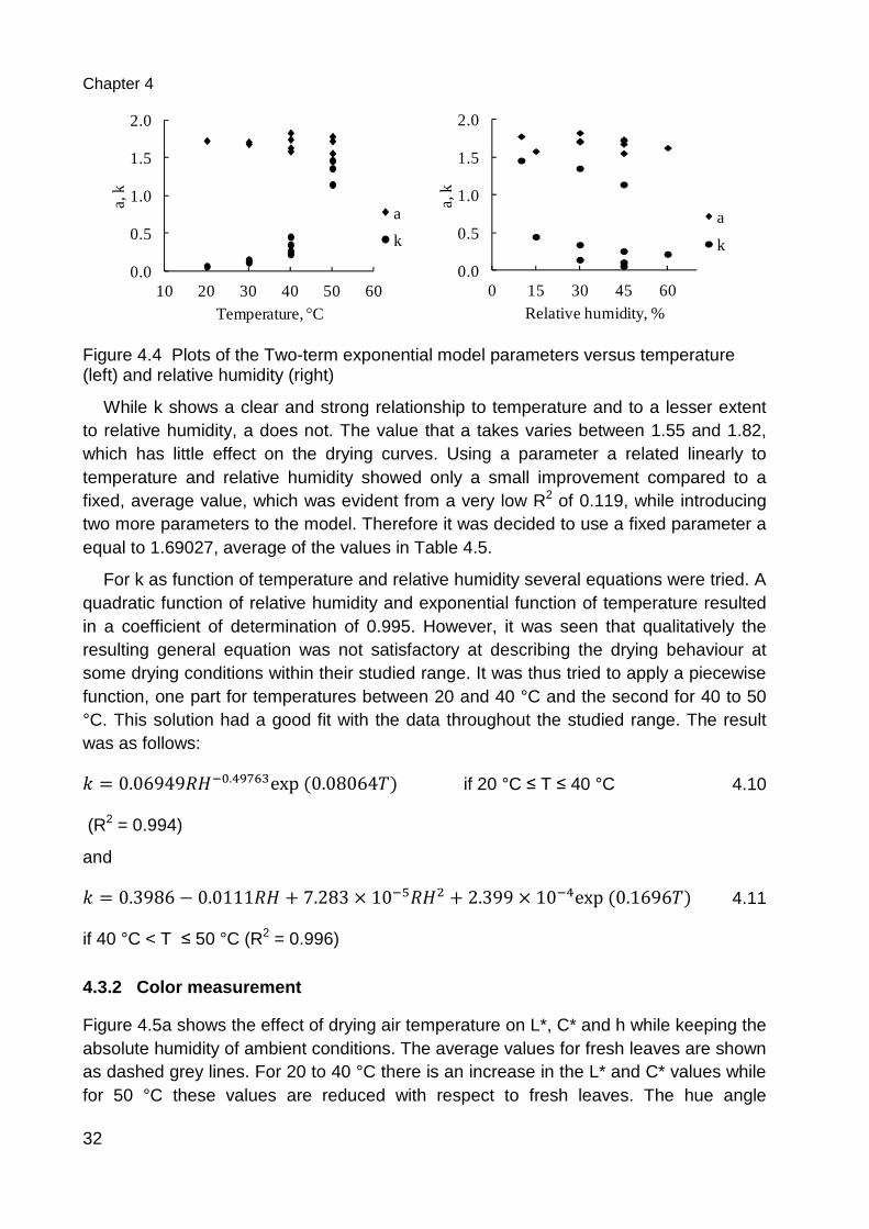
Figure 4.4 Plots of the Two-term exponential model parameters versus temperature (left) and relative humidity (right)

While k shows a clear and strong relationship to temperature and to a lesser extent to relative humidity, a does not. The value that a takes varies between 1.55 and 1.82, which has little effect on the drying curves. Using a parameter a related linearly to temperature and relative humidity showed only a small improvement compared to a fixed, average value, which was evident from a very low R2 of 0.119, while introducing two more parameters to the model. Therefore it was decided to use a fixed parameter a equal to 1.69027, average of the values in Table 4.5.

For k as function of temperature and relative humidity several equations were tried. A quadratic function of relative humidity and exponential function of temperature resulted in a coefficient of determination of 0.995. However, it was seen that qualitatively the resulting general equation was not satisfactory at describing the drying behaviour at some drying conditions within their studied range. It was thus tried to apply a piecewise function, one part for temperatures between 20 and 40 °C and the second for 40 to 50 °C. This solution had a good fit with the data throughout the studied range. The result was as follows: 1 = 0.06949� C?.:<DEFexp(0.08064)) if 20 °C ≤ T ≤ 40 °C 4.10

(R2 = 0.994)

and 1 = 0.3986 − 0.0111� + 7.283 × 10C;� ( + 2.399 × 10C:exp(0.1696)) 4.11

if 40 °C < T ≤ 50 °C (R2 = 0.996)

4.3.2 Color measurement

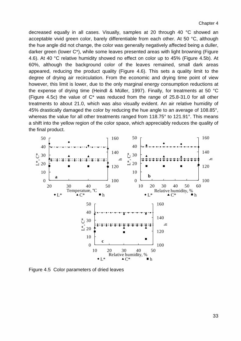
Figure 4.5a shows the effect of drying air temperature on L*, C* and h while keeping the absolute humidity of ambient conditions. The average values for fresh leaves are shown as dashed grey lines. For 20 to 40 °C there is an increase in the L* and C* values while for 50 °C these values are reduced with respect to fresh leaves. The hue angle

0.0

0.5

1.0

1.5

2.0

10 20 30 40 50 60

a, k

Temperature, °C

a

k

0.0

0.5

1.0

1.5

2.0

0 15 30 45 60

a, k

Relative humidity, %

a

k

Chapter 4

33

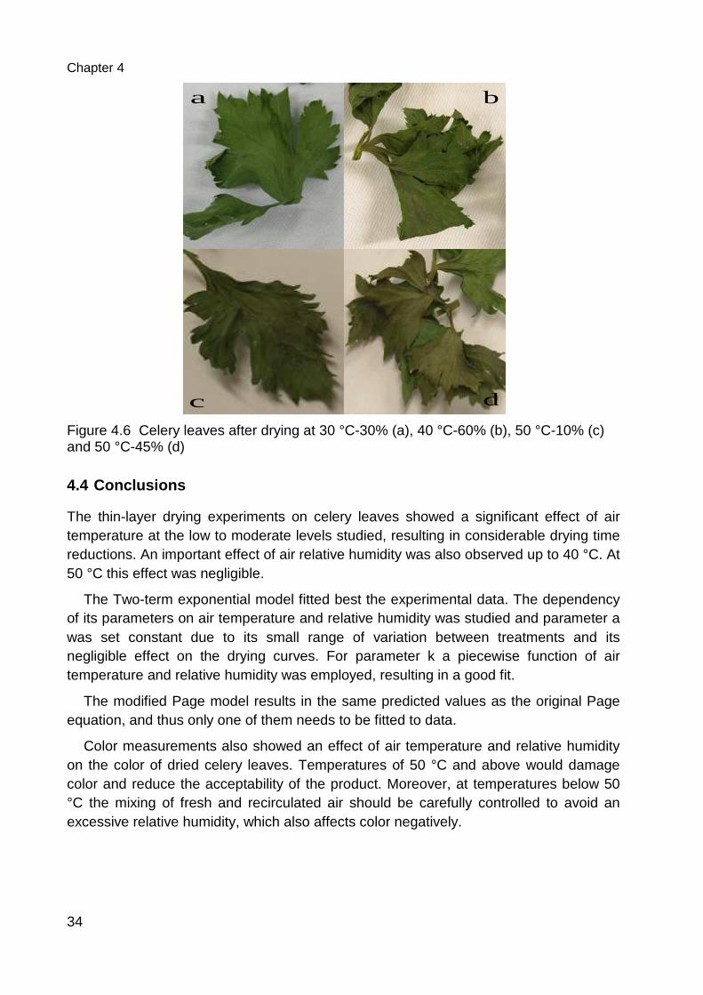
decreased equally in all cases. Visually, samples at 20 through 40 °C showed an acceptable vivid green color, barely differentiable from each other. At 50 °C, although the hue angle did not change, the color was generally negatively affected being a duller, darker green (lower C*), while some leaves presented areas with light browning (Figure 4.6). At 40 °C relative humidity showed no effect on color up to 45% (Figure 4.5b). At 60%, although the background color of the leaves remained, small dark areas appeared, reducing the product quality (Figure 4.6). This sets a quality limit to the degree of drying air recirculation. From the economic and drying time point of view however, this limit is lower, due to the only marginal energy consumption reductions at the expense of drying time (Heindl & Müller, 1997). Finally, for treatments at 50 °C (Figure 4.5c) the value of C* was reduced from the range of 25.8-31.0 for all other treatments to about 21.0, which was also visually evident. An air relative humidity of 45% drastically damaged the color by reducing the hue angle to an average of 108.85°, whereas the value for all other treatments ranged from 118.75° to 121.91°. This means a shift into the yellow region of the color space, which appreciably reduces the quality of the final product.

Figure 4.5 Color parameters of dried leaves

100

120

140

160

0

10

20

30

40

50

20 30 40 50

h

L*, C

*

Temperature, °CL* C* h

a100

120

140

160

0

10

20

30

40

50

10 20 30 40 50 60

h

L*, C

*

Relative humidity, %L* C* h

b

100

120

140

160

0

10

20

30

40

50

10 20 30 40 50

h

L*, C

*

Relative humidity, %L* C* h

c

Chapter 4

34

Figure 4.6 Celery leaves after drying at 30 °C-30% (a), 40 °C-60% (b), 50 °C-10% (c) and 50 °C-45% (d)

4.4 Conclusions

The thin-layer drying experiments on celery leaves showed a significant effect of air temperature at the low to moderate levels studied, resulting in considerable drying time reductions. An important effect of air relative humidity was also observed up to 40 °C. At 50 °C this effect was negligible.

The Two-term exponential model fitted best the experimental data. The dependency of its parameters on air temperature and relative humidity was studied and parameter a was set constant due to its small range of variation between treatments and its negligible effect on the drying curves. For parameter k a piecewise function of air temperature and relative humidity was employed, resulting in a good fit.

The modified Page model results in the same predicted values as the original Page equation, and thus only one of them needs to be fitted to data.

Color measurements also showed an effect of air temperature and relative humidity on the color of dried celery leaves. Temperatures of 50 °C and above would damage color and reduce the acceptability of the product. Moreover, at temperatures below 50 °C the mixing of fresh and recirculated air should be carefully controlled to avoid an excessive relative humidity, which also affects color negatively.

a b

c d

35

5 Improvement of air distribution in a fixed-bed dryer using computational fluid dynamics

Uneven air distribution is a major problem in the performance of batch dryers. Zones receiving a higher airflow rate dry faster, and this heterogeneity reduces efficiency by increasing energy consumption and drying time. A simple box dryer with 36 boxes placed over the plenum chamber was built and tested and computational fluid dynamics was used to simulate its air distribution.

Simulations showed that this configuration produced a poor air distribution. Trying to overcome this problem, simulations were conducted with a modified design consisting of a wide inlet into the plenum. Results showed an almost perfectly uniform air distribution. This was considered satisfactory for further study, which consisted of finding a suitable transition between the small cross section of the air ducts and the wide entrance to the plenum. It was seen, from theory and flow simulations that diffusers need to be prohibitively long to function properly. However, short, wide-angle diffusers can be equipped with air guides and perforated plates to remain effective.

Drying trials with woodchips were conducted for the original and modified dryer configurations, during which the drying course and airflow of each box were measured. Results for the original configuration showed, like the simulations, that there was a wide variation in airflow among the boxes, and also the expected wide differences in drying rate. A very significant correlation between these two variables was found. The modified version resulted in much more homogenous air distribution and drying rates and therefore represents a viable approach to improve dryer performance.

5.1 Introduction

Drying is an important post-harvest operation for the preservation of many agricultural products. When drying is part of the post-harvest process chain, it is usually the most energy- and cost-intensive operation.

For herbs and spices as well as for other products, fixed-bed batch dryers are widely used. This is mainly due to their relative ease of construction and the consequently low investment costs, which would allow small to medium size farms to construct their own dryers (Noetzel, 2006).

Fixed-bed dryers consist of a plenum chamber over which a grated false floor and walls stand to contain a bed of product. A fan is connected to the plenum chamber to force the air through either directly or using a duct system. Air is usually heated to increase the drying rate.

These dryers present a number of disadvantages and problems. One important disadvantage is that they usually have a high specific energy consumption. The main causes of this are the non-uniform drying and heat losses due to uneven flow distribution, non-uniform product distribution (bulk density and height), inefficient use of

Chapter 5

36

the drying potential of drying air, heat losses through air ducts and other dryer parts, and the absence of process control and instrumentation (Mellmann & Fürll, 2008). This paper aims to address the first of these causes, namely, the non-uniform distribution of drying air.

Studies on thin-layer drying of agricultural products have mostly shown that the velocity of drying air has no significant effect on the drying rate (Madamba et al., 1996; Müller & Heindl, 2006; Phupaichitkun, 2008). However, in fixed-bed dryers layers thicker than a few centimetres are used, and in these cases the airflow acts as a limiting factor for the drying rate. Here the air gets gradually saturated and colder in its way through the product layer and its drying potential is therefore gradually reduced, and the extent of this change depends on the amount of air flowing through (Kröll, 1978; Müller & Heindl, 2006). Thus, drying time is a function of airflow rate and an uneven air distribution leads to uneven drying (Brooker et al., 1992).

Uneven air distribution in fixed-bed dryers and others of similar characteristics has been reported for a variety of products in the literature (Brooker et al., 1992; Janjai et al., 2006; Jayas & Muir, 2002; Kröll, 1997; Mellmann & Fürll, 2008; Nagle et al., 2008; Noetzel, 2006; Rossrucker, 1973; Rumsey & Fortis, 1984). An air stream tends to keep its direction, and when it reaches an obstacle (a dryer wall for instance) it will be deflected upwards and to the side. The product above this region receives more air. Commonly used air inlets to the plenum chamber create a vortex close to the dryer walls, which in turn causes more rapid drying to occur there than at the centre (Rossrucker, 1973).

High air velocities from the fan cause high turbulence in the plenum chamber which favours the flow of air through some regions. Also, as the air enters the plenum, its velocity decreases due to the increased volume available and because air begins to flow through the product. As the air flows away from the entrance and air velocity decreases, there is a velocity pressure regain in the form of static pressure, which increases the flow of air in the opposite end of the dryer relative to the fan (Brooker et al., 1992; Jayas & Muir, 2002).

Some suggestions that have been given to improve this situation include: (a) the use of several air inlets, (b) the introduction of guides to deflect air, (c) the reduction in the cross-sectional area of the plenum chamber from the fan side to the opposite side, (d) the use of an adequate transition duct at the entrance to the plenum chamber which slows down the air.

The inclusion of several inlets would require additional fans or at least a complicated air duct system to deliver air from one fan to them. The use of air guides has been researched by Janjai et al. (2006) in a fixed-bed dryer for longan, and they reported an improvement in the air and temperature distribution, as well as in the uniformity of drying. However this seems difficult to transfer to dryers of different geometries, aspect ratios and sizes.

Chapter 5

37

The objective of this work was to study the air distribution in a fixed-bed dryer both experimentally and by using computational fluid dynamics (CFD), to measure its effect on drying uniformity and to find a simple modification to the dryer which improves uniformity.

5.2 Materials and methods

5.2.1 Description of the dryer

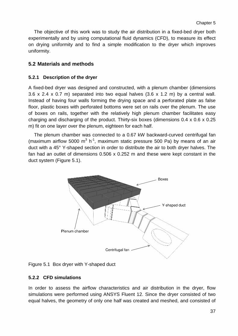
A fixed-bed dryer was designed and constructed, with a plenum chamber (dimensions 3.6 x 2.4 x 0.7 m) separated into two equal halves (3.6 x 1.2 m) by a central wall. Instead of having four walls forming the drying space and a perforated plate as false floor, plastic boxes with perforated bottoms were set on rails over the plenum. The use of boxes on rails, together with the relatively high plenum chamber facilitates easy charging and discharging of the product. Thirty-six boxes (dimensions 0.4 x 0.6 x 0.25 m) fit on one layer over the plenum, eighteen for each half.

The plenum chamber was connected to a 0.67 kW backward-curved centrifugal fan (maximum airflow 5000 m3 h-1, maximum static pressure 500 Pa) by means of an air duct with a 45° Y-shaped section in order to distribute the air to both dryer halves. The fan had an outlet of dimensions 0.506 x 0.252 m and these were kept constant in the duct system (Figure 5.1).

Figure 5.1 Box dryer with Y-shaped duct

5.2.2 CFD simulations

In order to assess the airflow characteristics and air distribution in the dryer, flow simulations were performed using ANSYS Fluent 12. Since the dryer consisted of two equal halves, the geometry of only one half was created and meshed, and consisted of

Chapter 5

38

about five hundred thousand cells. The simulations were done in steady state and the k-epsilon realisable turbulence model was employed. Air velocities in the system result in Mach numbers much smaller than 0.1, so the fluid was considered incompressible and a constant air density was employed (ANSYS, 2009). Air viscosity was also set constant.

Since only one half of the dryer was simulated, the air inlet into the geometry was taken as half the fan outlet. It was noticed, though, that the fan impeller was shifted to one side of its housing and therefore produced a very non-uniform velocity profile, which could significantly influence the flow. Therefore, a grid measurement of air velocity was carried out at the fan outlet with a Schiltknecht MiniAir2 vane anemometer with a probe diameter of 22 mm. The measurement grid was done using the trivial method. For this, the fan outlet cross section was divided into sixty four equal areas (8 x 8), and the air velocity was measured at their centroids using the averaging function of the device over an interval of twenty seconds. In the dryer geometry, the inlet was then divided into thirty two equal areas and, depending on which dryer half was being simulated, their respective air velocity values were entered as normal to the cross section. These values were proportionately varied according to the desired airflow rate.

To simulate the airflow resistance of the material to be dried (woodchips) the porous media model was used (ANSYS, 2009). This requires the input of two resistance coefficients (viscous and inertial) to model the pressure drop per unit thickness caused by the product bulk, and they were obtained by fitting a second order polynomial function with zero intercept to pressure drop data collected by Suggs & Lanier (1985). Since it was not possible for this study to make a size characterisation and classification of the woodchip material, the data used corresponded to woodchips of mixed size. The airflow resistance was considered to be isotropic. Also, although difficult to attain in practice, it was assumed for the simulations that all boxes imposed the exact same resistance to airflow, in order to evaluate only the effect of the dryer configuration on the air distribution. Measurements showed that the pressure drop caused by the boxes’ perforated floors was negligible at the dryer’s working conditions.

Simulations were run until the scaled residuals’ curves were horizontal, which occurred at a maximum value of 6.3 x10-5 and usually lower, complying with the default convergence criterion in Fluent of 1x10-3 (ANSYS, 2009).

5.2.3 Drying tests

In order to measure air distribution and drying uniformity, three drying trials (trials one to three) were performed on the original dryer configuration detailed above and three more (trials four to six) after its modification (see section 5.3.1). The product to be dried was woodchips with an average initial moisture content of 52% (wet basis). Before loading the boxes, the fresh product was thoroughly mixed. For the first trial of both configurations (trials one and four), boxes were filled up to the top with fresh product. For the rest they were half filled. The initial weight of all boxes was the same within

Chapter 5

39

each trial. Two gas burners with a total maximum power of 60 kW were positioned at the fan inlet to heat up ambient air to 50-65 °C.

Figure 5.2 shows a diagram of the experimental set-up. Each drying trial consisted of several periods of 1.5 h. After each period all boxes were taken down simultaneously from the dryer and weighed on a Sartorius MC1 IC 34000P scale with a resolution of 0.1 g. During each period, the relative airflow rate through each box was measured. For this, a tapered channel was used to accelerate the air (Navarro & Noyes, 2002; Olver & Clyde, 1950; Parker et al., 1992). The large end of the tapered channel had the same cross section dimensions as the boxes to collect all the air flowing through them, and its opposite side had dimensions 0.17 x 0.11 m. This gradual contraction would bring a more uniform air distribution at the outlet cross section (Kröll, 1997), where an Airflow TA5 hot-wire anemometer with a resolution of 0.01 m s-1 was placed at the centre to measure air velocity. Thus, the velocity so measured was considered to be a good indicator of the relative airflow rate.

Figure 5.2 Experimental set-up of drying trials

5.3 Results and discussion

5.3.1 CFD simulations

Figure 5.3a shows flow pathlines, their colour representing air velocity. The sudden expansion into the plenum chamber allows the drying air to maintain its high velocity. The metal frame of the plenum walls and the walls themselves create obstacles to the air, forcing it to change its direction drastically and forming vortices. This flow produces differences in static pressure under the boxes, which favour the flow of air through some locations over others (Rossrucker, 1973).

Figure 5.3b shows contours of velocity in the vertical direction halfway through the boxes for the right half of the dryer. The airflow through the dryer was fixed at 0.648 m3

s -1, which for the dryer dimensions corresponds to an average superficial air velocity

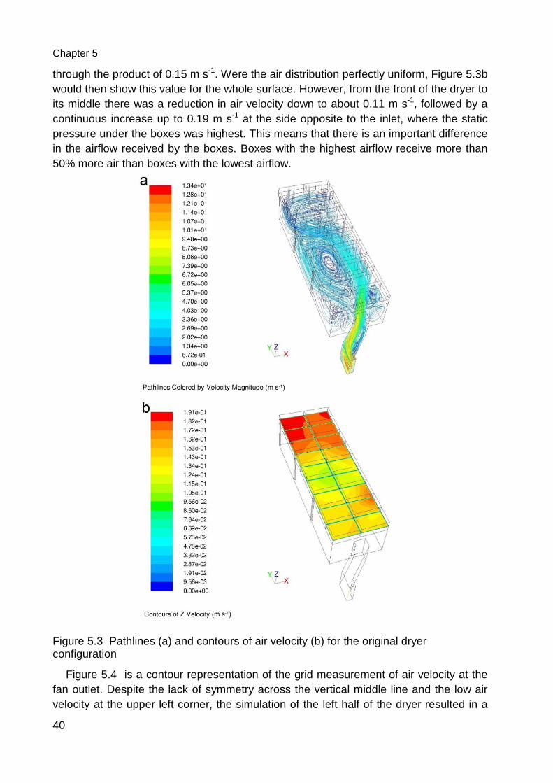
Chapter 5

40

through the product of 0.15 m s-1. Were the air distribution perfectly uniform, Figure 5.3b would then show this value for the whole surface. However, from the front of the dryer to its middle there was a reduction in air velocity down to about 0.11 m s-1, followed by a continuous increase up to 0.19 m s-1 at the side opposite to the inlet, where the static pressure under the boxes was highest. This means that there is an important difference in the airflow received by the boxes. Boxes with the highest airflow receive more than 50% more air than boxes with the lowest airflow.

Figure 5.3 Pathlines (a) and contours of air velocity (b) for the original dryer configuration

Figure 5.4 is a contour representation of the grid measurement of air velocity at the fan outlet. Despite the lack of symmetry across the vertical middle line and the low air velocity at the upper left corner, the simulation of the left half of the dryer resulted in a

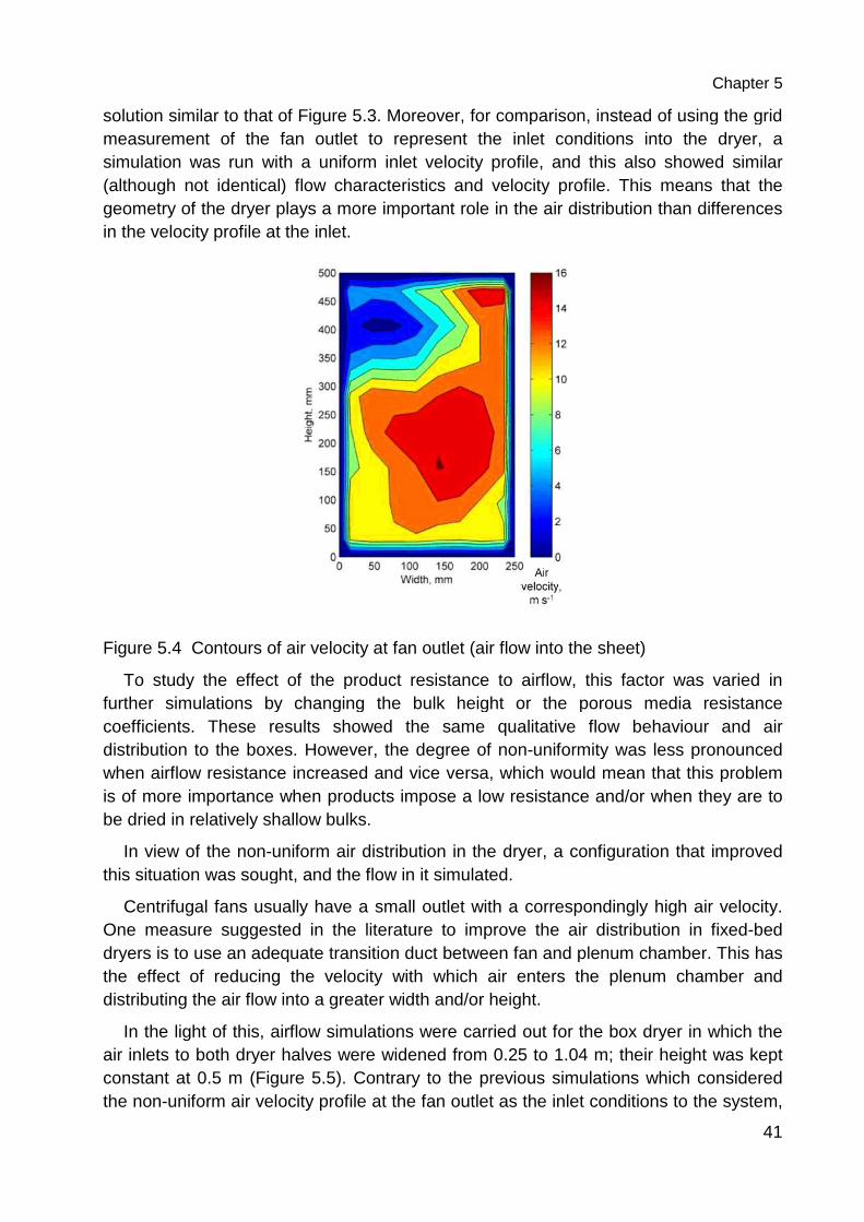
solution similar to that of Figure measurement of the fan outlet to represent the inlet conditions into the dryer, a simulation was run with a uniform inlet v(although not identical) flow characteristics and velocity profile. This means that the geometry of the dryer plays a more important role in the air distribution than differences in the velocity profile at the

Figure 5.4 Contours of air velocity at fan outlet (air flow into the sheet)

To study the effect of the product resistance to airflow, this factor was varied in further simulations by changing the bucoefficients. These results showed the same qualitative flow behaviour and air distribution to the boxes. However, the degree of nonwhen airflow resistance increased and vice versa, wis of more importance when products impose a low resistance and/or when they are to be dried in relatively shallow bulks.

In view of the non-uniform air distribution in the dryer, a configuration that improved this situation was sought, and the flow in it simulated.

Centrifugal fans usually have a small outlet with a correspondingly high air velocity. One measure suggested in the literature to improve the air distribution in fixeddryers is to use an adequate transitiothe effect of reducing the velocity with which air enters the plenum chamber and distributing the air flow into a greater width and/or height.

In the light of this, airflow simulations were carried out for thair inlets to both dryer halves were widened from 0.25 to 1.04 m; their height was kept constant at 0.5 m (Figure 5the non-uniform air velocity profile at the fan outlet as the inlet conditions to the system,

Figure 5.3. Moreover, for comparison, instead of using the grid measurement of the fan outlet to represent the inlet conditions into the dryer, a simulation was run with a uniform inlet velocity profile, and this also showed similar (although not identical) flow characteristics and velocity profile. This means that the geometry of the dryer plays a more important role in the air distribution than differences in the velocity profile at the inlet.

Contours of air velocity at fan outlet (air flow into the sheet)

To study the effect of the product resistance to airflow, this factor was varied in further simulations by changing the bulk height or the porous media resistance coefficients. These results showed the same qualitative flow behaviour and air distribution to the boxes. However, the degree of non-uniformity was less pronounced when airflow resistance increased and vice versa, which would mean that this problem is of more importance when products impose a low resistance and/or when they are to be dried in relatively shallow bulks.

uniform air distribution in the dryer, a configuration that improved on was sought, and the flow in it simulated.

Centrifugal fans usually have a small outlet with a correspondingly high air velocity. One measure suggested in the literature to improve the air distribution in fixeddryers is to use an adequate transition duct between fan and plenum chamber. This has the effect of reducing the velocity with which air enters the plenum chamber and distributing the air flow into a greater width and/or height.

In the light of this, airflow simulations were carried out for the box dryer in which the air inlets to both dryer halves were widened from 0.25 to 1.04 m; their height was kept

5.5). Contrary to the previous simulations which considered velocity profile at the fan outlet as the inlet conditions to the system,

Chapter 5

41

. Moreover, for comparison, instead of using the grid measurement of the fan outlet to represent the inlet conditions into the dryer, a

elocity profile, and this also showed similar (although not identical) flow characteristics and velocity profile. This means that the geometry of the dryer plays a more important role in the air distribution than differences

Contours of air velocity at fan outlet (air flow into the sheet)

To study the effect of the product resistance to airflow, this factor was varied in lk height or the porous media resistance

coefficients. These results showed the same qualitative flow behaviour and air uniformity was less pronounced

hich would mean that this problem is of more importance when products impose a low resistance and/or when they are to

uniform air distribution in the dryer, a configuration that improved

Centrifugal fans usually have a small outlet with a correspondingly high air velocity. One measure suggested in the literature to improve the air distribution in fixed-bed

n duct between fan and plenum chamber. This has the effect of reducing the velocity with which air enters the plenum chamber and

e box dryer in which the air inlets to both dryer halves were widened from 0.25 to 1.04 m; their height was kept

). Contrary to the previous simulations which considered velocity profile at the fan outlet as the inlet conditions to the system,

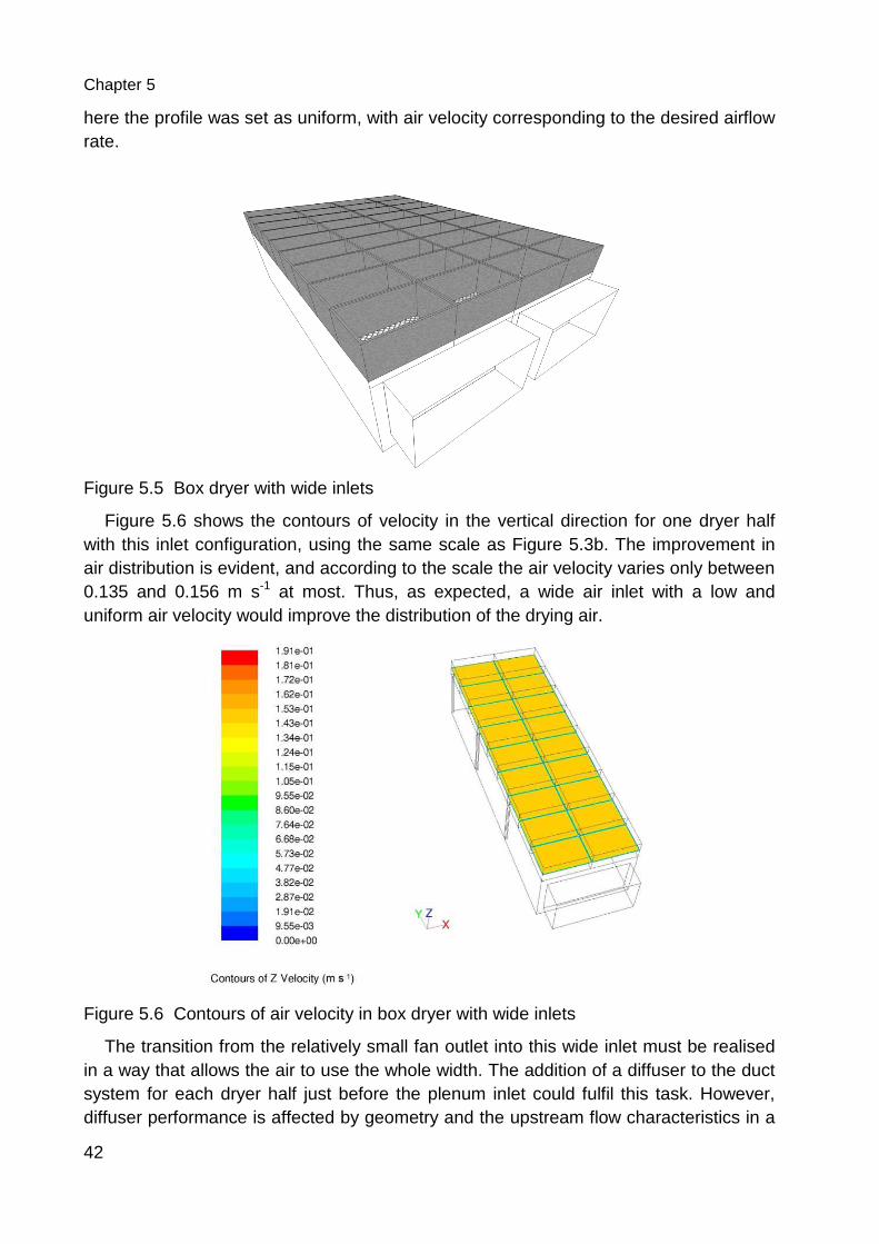
Chapter 5

42

here the profile was set as uniform, with air velocity corresponding to the desired airflow rate.

Figure 5.5 Box dryer with wide inlets

Figure 5.6 shows the contours of velocity in the vertical direction for one dryer half with this inlet configuration, using the same scale as Figure 5.3b. The improvement in air distribution is evident, and according to the scale the air velocity varies only between 0.135 and 0.156 m s-1 at most. Thus, as expected, a wide air inlet with a low and uniform air velocity would improve the distribution of the drying air.

Figure 5.6 Contours of air velocity in box dryer with wide inlets

The transition from the relatively small fan outlet into this wide inlet must be realised in a way that allows the air to use the whole width. The addition of a diffuser to the duct system for each dryer half just before the plenum inlet could fulfil this task. However, diffuser performance is affected by geometry and the upstream flow characteristics in a

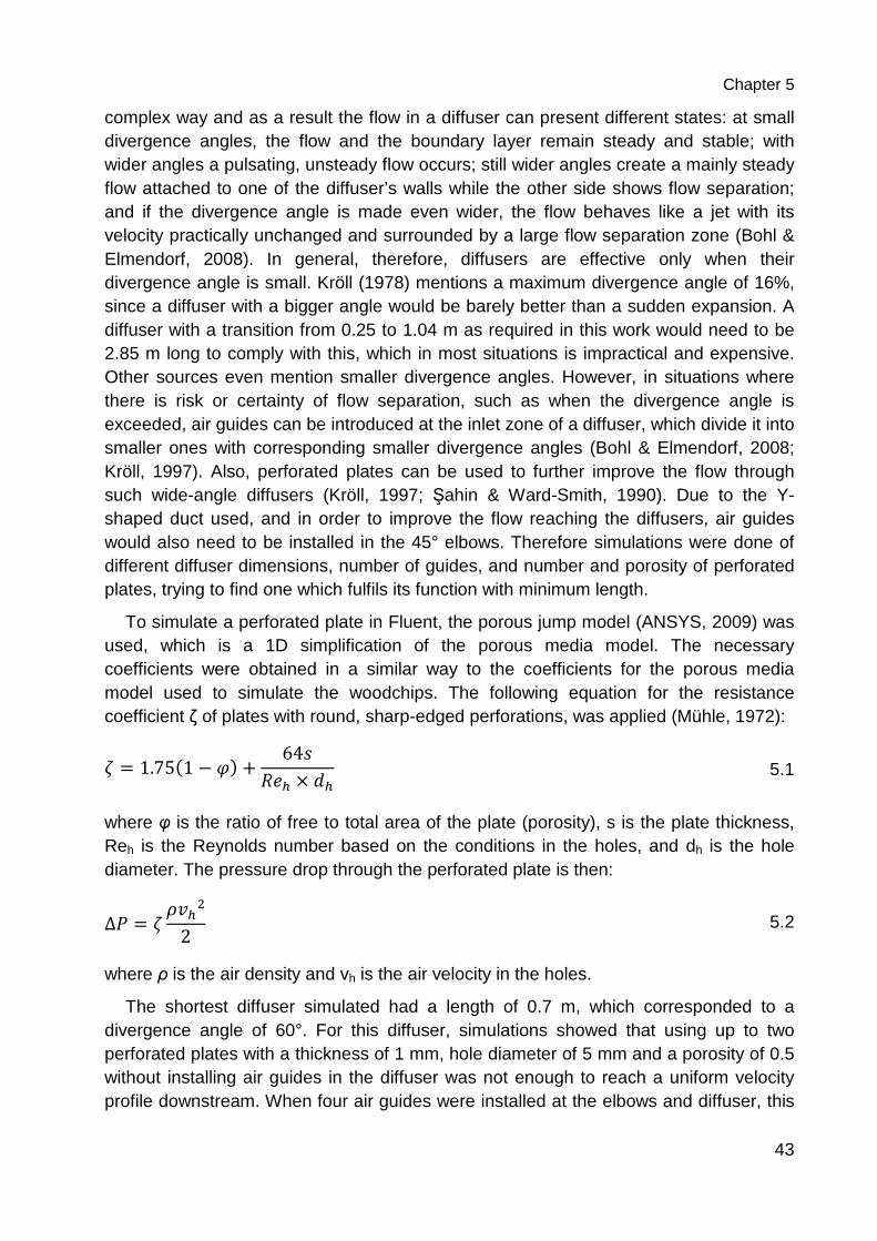
Chapter 5

43

complex way and as a result the flow in a diffuser can present different states: at small divergence angles, the flow and the boundary layer remain steady and stable; with wider angles a pulsating, unsteady flow occurs; still wider angles create a mainly steady flow attached to one of the diffuser’s walls while the other side shows flow separation; and if the divergence angle is made even wider, the flow behaves like a jet with its velocity practically unchanged and surrounded by a large flow separation zone (Bohl & Elmendorf, 2008). In general, therefore, diffusers are effective only when their divergence angle is small. Kröll (1978) mentions a maximum divergence angle of 16%, since a diffuser with a bigger angle would be barely better than a sudden expansion. A diffuser with a transition from 0.25 to 1.04 m as required in this work would need to be 2.85 m long to comply with this, which in most situations is impractical and expensive. Other sources even mention smaller divergence angles. However, in situations where there is risk or certainty of flow separation, such as when the divergence angle is exceeded, air guides can be introduced at the inlet zone of a diffuser, which divide it into smaller ones with corresponding smaller divergence angles (Bohl & Elmendorf, 2008; Kröll, 1997). Also, perforated plates can be used to further improve the flow through such wide-angle diffusers (Kröll, 1997; Şahin & Ward-Smith, 1990). Due to the Y-shaped duct used, and in order to improve the flow reaching the diffusers, air guides would also need to be installed in the 45° elbows. Therefore simulations were done of different diffuser dimensions, number of guides, and number and porosity of perforated plates, trying to find one which fulfils its function with minimum length.

To simulate a perforated plate in Fluent, the porous jump model (ANSYS, 2009) was used, which is a 1D simplification of the porous media model. The necessary coefficients were obtained in a similar way to the coefficients for the porous media model used to simulate the woodchips. The following equation for the resistance coefficient ζ of plates with round, sharp-edged perforations, was applied (Mühle, 1972):

J = 1.75(1 − K) + 64L�+M × *M 5.1

where φ is the ratio of free to total area of the plate (porosity), s is the plate thickness, Reh is the Reynolds number based on the conditions in the holes, and dh is the hole diameter. The pressure drop through the perforated plate is then:

∆O = J PQM(2 5.2

where ρ is the air density and vh is the air velocity in the holes.

The shortest diffuser simulated had a length of 0.7 m, which corresponded to a divergence angle of 60°. For this diffuser, simulations showed that using up to two perforated plates with a thickness of 1 mm, hole diameter of 5 mm and a porosity of 0.5 without installing air guides in the diffuser was not enough to reach a uniform velocity profile downstream. When four air guides were installed at the elbows and diffuser, this

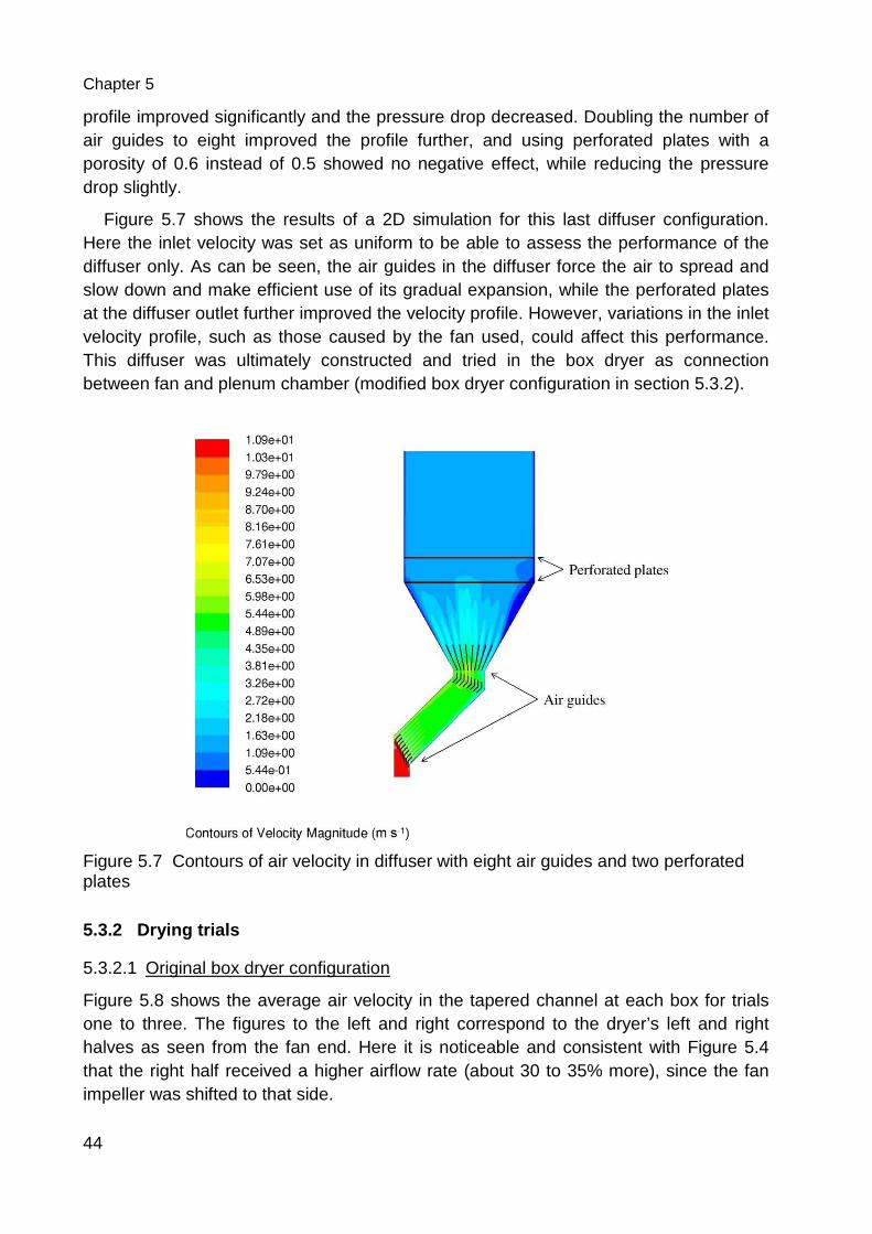
Chapter 5

44

profile improved significantly and the pressure drop decreased. Doubling the number of air guides to eight improved the profile further, and using perforated plates with a porosity of 0.6 instead of 0.5 showed no negative effect, while reducing the pressure drop slightly.

Figure 5.7 shows the results of a 2D simulation for this last diffuser configuration. Here the inlet velocity was set as uniform to be able to assess the performance of the diffuser only. As can be seen, the air guides in the diffuser force the air to spread and slow down and make efficient use of its gradual expansion, while the perforated plates at the diffuser outlet further improved the velocity profile. However, variations in the inlet velocity profile, such as those caused by the fan used, could affect this performance. This diffuser was ultimately constructed and tried in the box dryer as connection between fan and plenum chamber (modified box dryer configuration in section 5.3.2).

Figure 5.7 Contours of air velocity in diffuser with eight air guides and two perforated plates

5.3.2 Drying trials

5.3.2.1 Original box dryer configuration

Figure 5.8 shows the average air velocity in the tapered channel at each box for trials one to three. The figures to the left and right correspond to the dryer’s left and right halves as seen from the fan end. Here it is noticeable and consistent with Figure 5.4 that the right half received a higher airflow rate (about 30 to 35% more), since the fan impeller was shifted to that side.

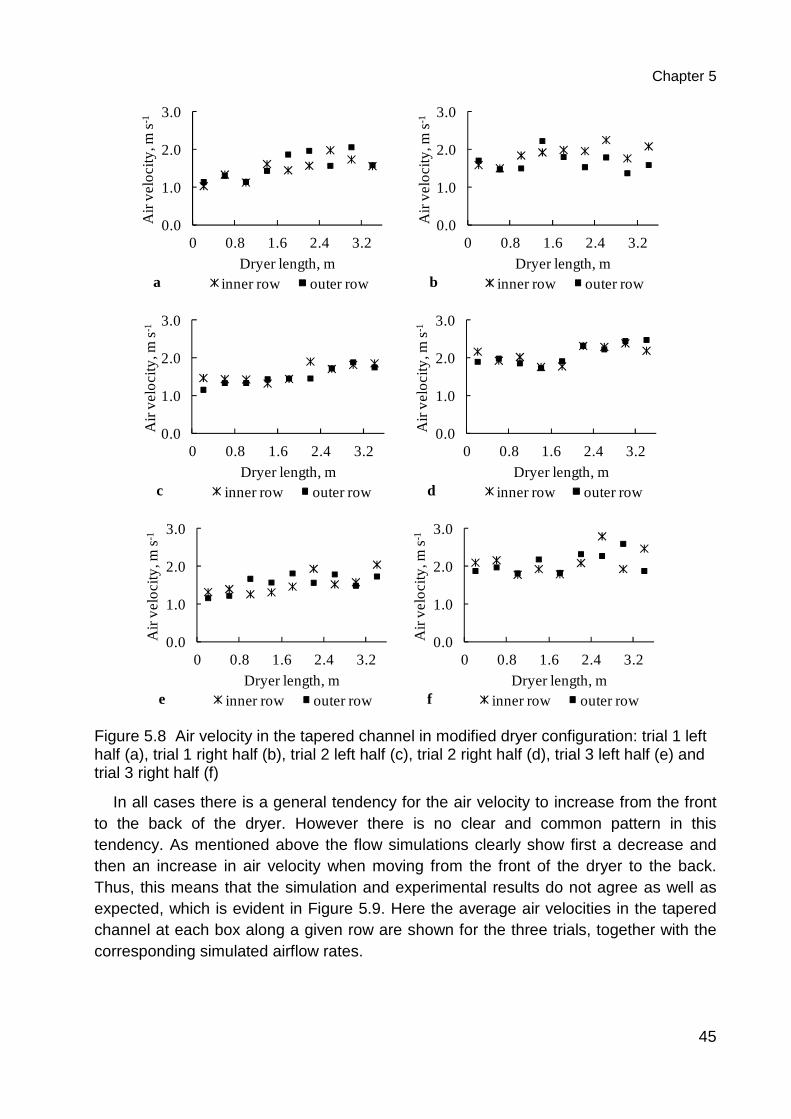
Chapter 5

45

Figure 5.8 Air velocity in the tapered channel in modified dryer configuration: trial 1 left half (a), trial 1 right half (b), trial 2 left half (c), trial 2 right half (d), trial 3 left half (e) and trial 3 right half (f)

In all cases there is a general tendency for the air velocity to increase from the front to the back of the dryer. However there is no clear and common pattern in this tendency. As mentioned above the flow simulations clearly show first a decrease and then an increase in air velocity when moving from the front of the dryer to the back. Thus, this means that the simulation and experimental results do not agree as well as expected, which is evident in Figure 5.9. Here the average air velocities in the tapered channel at each box along a given row are shown for the three trials, together with the corresponding simulated airflow rates.

0.0

1.0

2.0

3.0

0 0.8 1.6 2.4 3.2

Air

velo

city

, m s-

1

Dryer length, minner row outer rowa

0.0

1.0

2.0

3.0

0 0.8 1.6 2.4 3.2

Air

velo

city

, m s-

1

Dryer length, minner row outer rowb

0.0

1.0

2.0

3.0

0 0.8 1.6 2.4 3.2

Air

velo

city

, m s-

1

Dryer length, minner row outer rowc

0.0

1.0

2.0

3.0

0 0.8 1.6 2.4 3.2

Air

velo

city

, m s-

1

Dryer length, minner row outer rowd

0.0

1.0

2.0

3.0

0 0.8 1.6 2.4 3.2

Air

velo

city

, m s-

1

Dryer length, minner row outer rowe

0.0

1.0

2.0

3.0

0 0.8 1.6 2.4 3.2

Air

velo

city

, m s-

1

Dryer length, minner row outer rowf

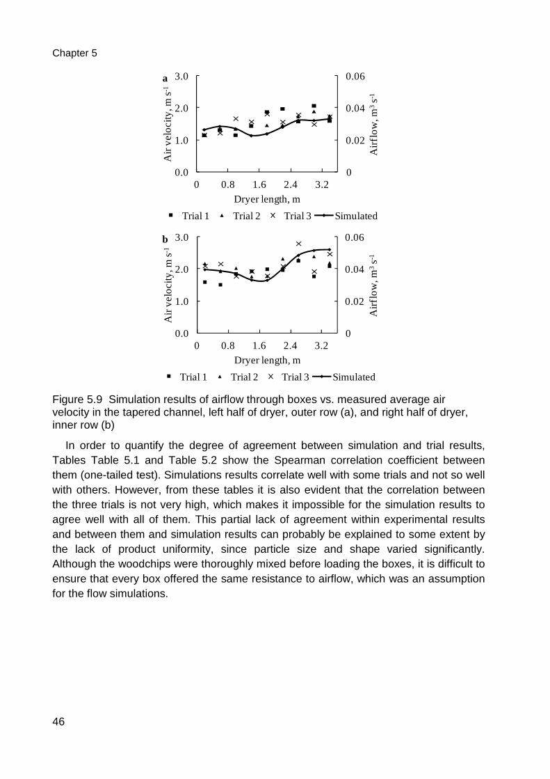
Chapter 5

46

Figure 5.9 Simulation results of airflow through boxes vs. measured average air velocity in the tapered channel, left half of dryer, outer row (a), and right half of dryer, inner row (b)

In order to quantify the degree of agreement between simulation and trial results, Tables Table 5.1 and Table 5.2 show the Spearman correlation coefficient between them (one-tailed test). Simulations results correlate well with some trials and not so well with others. However, from these tables it is also evident that the correlation between the three trials is not very high, which makes it impossible for the simulation results to agree well with all of them. This partial lack of agreement within experimental results and between them and simulation results can probably be explained to some extent by the lack of product uniformity, since particle size and shape varied significantly. Although the woodchips were thoroughly mixed before loading the boxes, it is difficult to ensure that every box offered the same resistance to airflow, which was an assumption for the flow simulations.

0

0.02

0.04

0.06

0.0

1.0

2.0

3.0

0 0.8 1.6 2.4 3.2

Airf

low

, m3s-

1

Air

velo

city

, m s-

1

Dryer length, m

Trial 1 Trial 2 Trial 3 Simulated

a

0

0.02

0.04

0.06

0.0

1.0

2.0

3.0

0 0.8 1.6 2.4 3.2

Airf

low

, m3s-

1

Air

velo

city

, m s-

1

Dryer length, m

Trial 1 Trial 2 Trial 3 Simulated

b

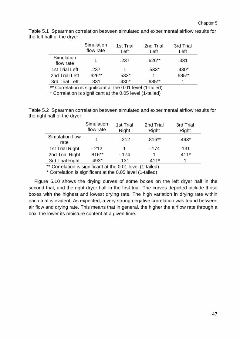
Chapter 5

47

Table 5.1 Spearman correlation between simulated and experimental airflow results for the left half of the dryer

Simulation flow rate

1st Trial Left

2nd Trial Left

3rd Trial Left

Simulation flow rate 1 .237 .626** .331

1st Trial Left .237 1 .533* .430* 2nd Trial Left .626** .533* 1 .685** 3rd Trial Left .331 .430* .685** 1 ** Correlation is significant at the 0.01 level (1-tailed) * Correlation is significant at the 0.05 level (1-tailed)

Table 5.2 Spearman correlation between simulated and experimental airflow results for the right half of the dryer

Simulation flow rate

1st Trial Right

2nd Trial Right

3rd Trial Right

Simulation flow rate 1 -.212 .816** .493*

1st Trial Right -.212 1 -.174 .131 2nd Trial Right .816** -.174 1 .411* 3rd Trial Right .493* .131 .411* 1

** Correlation is significant at the 0.01 level (1-tailed) * Correlation is significant at the 0.05 level (1-tailed)

Figure 5.10 shows the drying curves of some boxes on the left dryer half in the second trial, and the right dryer half in the first trial. The curves depicted include those boxes with the highest and lowest drying rate. The high variation in drying rate within each trial is evident. As expected, a very strong negative correlation was found between air flow and drying rate. This means that in general, the higher the airflow rate through a box, the lower its moisture content at a given time.

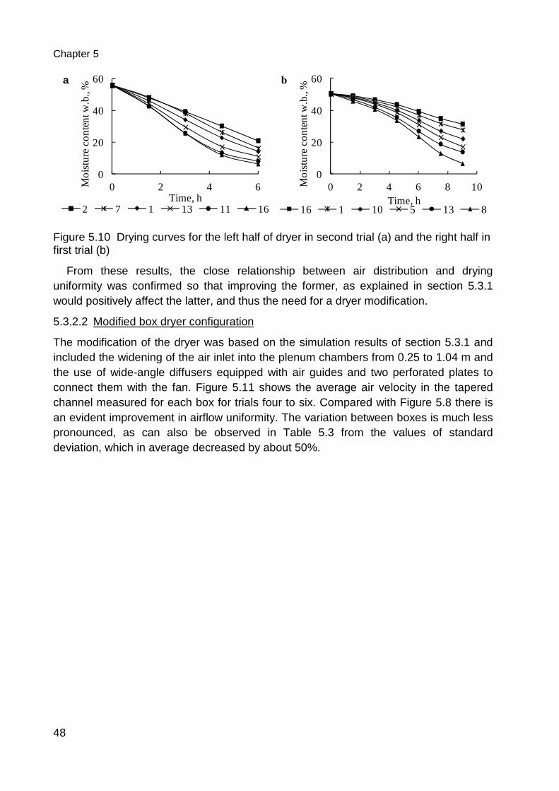
Chapter 5

48

Figure 5.10 Drying curves for the left half of dryer in second trial (a) and the right half in first trial (b)

From these results, the close relationship between air distribution and drying uniformity was confirmed so that improving the former, as explained in section 5.3.1 would positively affect the latter, and thus the need for a dryer modification.

5.3.2.2 Modified box dryer configuration

The modification of the dryer was based on the simulation results of section 5.3.1 and included the widening of the air inlet into the plenum chambers from 0.25 to 1.04 m and the use of wide-angle diffusers equipped with air guides and two perforated plates to connect them with the fan. Figure 5.11 shows the average air velocity in the tapered channel measured for each box for trials four to six. Compared with Figure 5.8 there is an evident improvement in airflow uniformity. The variation between boxes is much less pronounced, as can also be observed in Table 5.3 from the values of standard deviation, which in average decreased by about 50%.

0

20

40

60

0 2 4 6Mo

istu

re c

on

ten

t w.b

., %

Time, h2 7 1 13 11 16

a

0

20

40

60

0 2 4 6 8 10Mo

istu

re c

on

ten

t w.b

., %

Time, h16 1 10 5 13 8

b

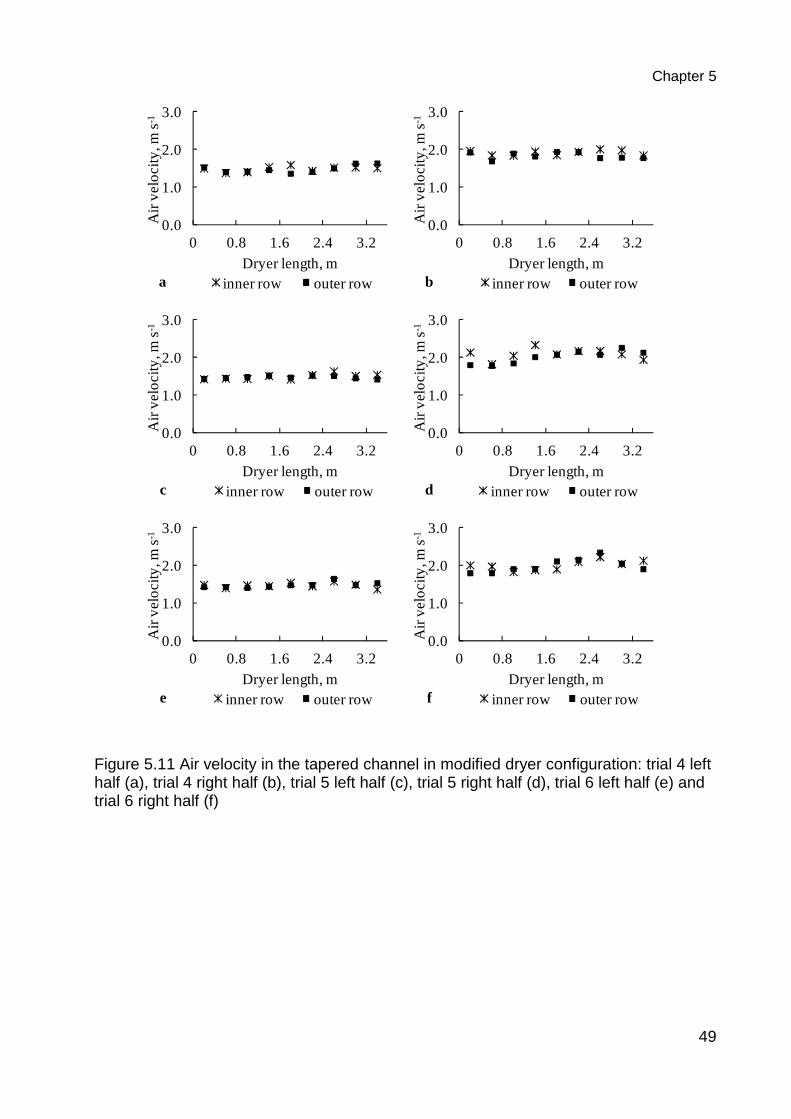
Chapter 5

49

Figure 5.11 Air velocity in the tapered channel in modified dryer configuration: trial 4 left half (a), trial 4 right half (b), trial 5 left half (c), trial 5 right half (d), trial 6 left half (e) and trial 6 right half (f)

0.0

1.0

2.0

3.0

0 0.8 1.6 2.4 3.2

Air

velo

city

, m s-

1

Dryer length, minner row outer rowa

0.0

1.0

2.0

3.0

0 0.8 1.6 2.4 3.2

Air

velo

city

, m s-

1

Dryer length, minner row outer rowb

0.0

1.0

2.0

3.0

0 0.8 1.6 2.4 3.2

Air

velo

city

, m s-

1

Dryer length, minner row outer rowc

0.0

1.0

2.0

3.0

0 0.8 1.6 2.4 3.2

Air

velo

city

, m s-

1

Dryer length, minner row outer rowd

0.0

1.0

2.0

3.0

0 0.8 1.6 2.4 3.2

Air

velo

city

, m s-

1

Dryer length, minner row outer rowe

0.0

1.0

2.0

3.0

0 0.8 1.6 2.4 3.2

Air

velo

city

, m s-

1

Dryer length, minner row outer rowf

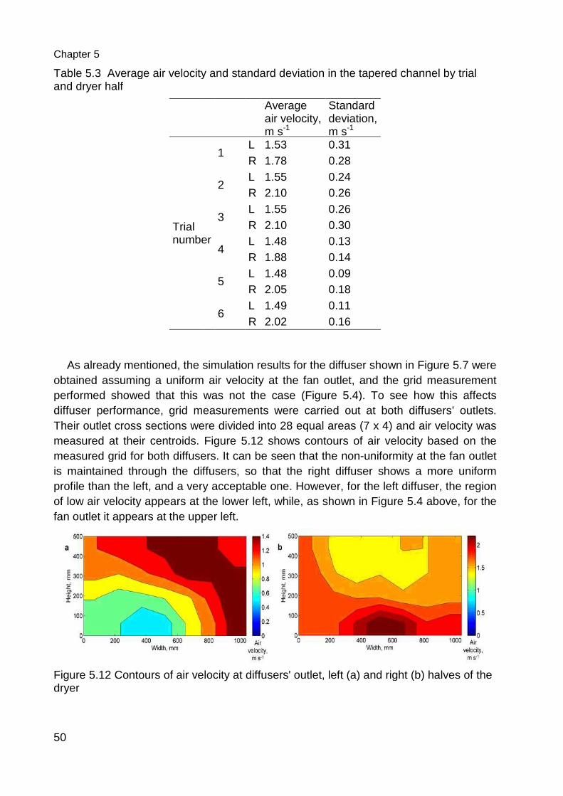
Chapter 5

50

Table 5.3 Average air velocity and standard deviation in the tapered channel by trial and dryer half

Trial number

As already mentioned, the simulation results for the diffuser shown in obtained assuming a uniform air velocity at the fan outlet, and the grid measurement performed showed that this was not the case (diffuser performance, grid measurements were Their outlet cross sections were divided into 28 equal areas (7 x 4) and air velocity was measured at their centroids. measured grid for both diffusers. It can be seen that the nonis maintained through the diffusers, so that the right diffuser shows a more uniform profile than the left, and a very acceptable one. However, for the left diffuser, tof low air velocity appears at the lower left, while, as shown in fan outlet it appears at the upper left.

Figure 5.12 Contours of air velodryer

Average air velocity and standard deviation in the tapered channel by trial

Average air velocity, m s-1

Standard deviation, m s-1

number

1 L 1.53 0.31 R 1.78 0.28

2 L 1.55 0.24 R 2.10 0.26

3 L 1.55 0.26 R 2.10 0.30

4 L 1.48 0.13 R 1.88 0.14

5 L 1.48 0.09 R 2.05 0.18

6 L 1.49 0.11 R 2.02 0.16

As already mentioned, the simulation results for the diffuser shown in obtained assuming a uniform air velocity at the fan outlet, and the grid measurement performed showed that this was not the case (Figure 5.4). To see how this affects diffuser performance, grid measurements were carried out at both diffusers’ outlets. Their outlet cross sections were divided into 28 equal areas (7 x 4) and air velocity was measured at their centroids. Figure 5.12 shows contours of air velocity based on the

sured grid for both diffusers. It can be seen that the non-uniformity at the fan outlet is maintained through the diffusers, so that the right diffuser shows a more uniform profile than the left, and a very acceptable one. However, for the left diffuser, tof low air velocity appears at the lower left, while, as shown in Figure 5fan outlet it appears at the upper left.

Contours of air velocity at diffusers' outlet, left (a) and right (b) halves of the

Average air velocity and standard deviation in the tapered channel by trial

As already mentioned, the simulation results for the diffuser shown in Figure 5.7 were obtained assuming a uniform air velocity at the fan outlet, and the grid measurement

). To see how this affects carried out at both diffusers’ outlets.

Their outlet cross sections were divided into 28 equal areas (7 x 4) and air velocity was shows contours of air velocity based on the

uniformity at the fan outlet is maintained through the diffusers, so that the right diffuser shows a more uniform profile than the left, and a very acceptable one. However, for the left diffuser, the region

5.4 above, for the

sers' outlet, left (a) and right (b) halves of the

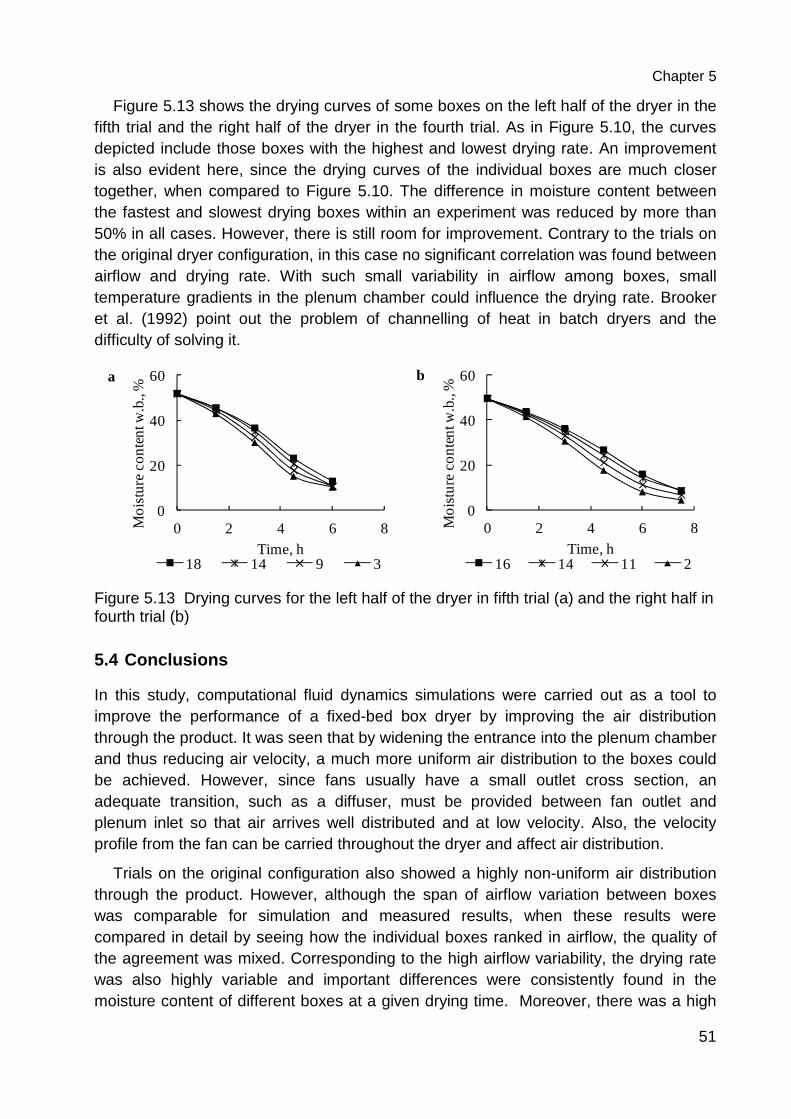
Chapter 5

51

Figure 5.13 shows the drying curves of some boxes on the left half of the dryer in the fifth trial and the right half of the dryer in the fourth trial. As in Figure 5.10, the curves depicted include those boxes with the highest and lowest drying rate. An improvement is also evident here, since the drying curves of the individual boxes are much closer together, when compared to Figure 5.10. The difference in moisture content between the fastest and slowest drying boxes within an experiment was reduced by more than 50% in all cases. However, there is still room for improvement. Contrary to the trials on the original dryer configuration, in this case no significant correlation was found between airflow and drying rate. With such small variability in airflow among boxes, small temperature gradients in the plenum chamber could influence the drying rate. Brooker et al. (1992) point out the problem of channelling of heat in batch dryers and the difficulty of solving it.

Figure 5.13 Drying curves for the left half of the dryer in fifth trial (a) and the right half in fourth trial (b)

5.4 Conclusions

In this study, computational fluid dynamics simulations were carried out as a tool to improve the performance of a fixed-bed box dryer by improving the air distribution through the product. It was seen that by widening the entrance into the plenum chamber and thus reducing air velocity, a much more uniform air distribution to the boxes could be achieved. However, since fans usually have a small outlet cross section, an adequate transition, such as a diffuser, must be provided between fan outlet and plenum inlet so that air arrives well distributed and at low velocity. Also, the velocity profile from the fan can be carried throughout the dryer and affect air distribution.

Trials on the original configuration also showed a highly non-uniform air distribution through the product. However, although the span of airflow variation between boxes was comparable for simulation and measured results, when these results were compared in detail by seeing how the individual boxes ranked in airflow, the quality of the agreement was mixed. Corresponding to the high airflow variability, the drying rate was also highly variable and important differences were consistently found in the moisture content of different boxes at a given drying time. Moreover, there was a high

0

20

40

60

0 2 4 6 8Mo

istu

re c

on

ten

t w.b

., %

Time, h18 14 9 3

a

0

20

40

60

0 2 4 6 8Mo

istu

re c

on

ten

t w.b

., %

Time, h16 14 11 2

b

Chapter 5

52

correlation between the airflow through a given box and its drying rate, from which it was expected that a better air distribution would improve drying uniformity.

Measurements of air velocity in the tapered channel showed that the modified dryer configuration resulted in a significantly more homogenous air distribution. This translated into more uniform drying of the product. The span of moisture content between boxes at a given time was reduced by more than 50% compared to the original dryer configuration. Thus, the proposed modifications provide a simple way to improve the performance of both existing and new fixed-bed dryers.

53

6 Numerical simulations and experimental measurements on the distribution of air and drying of round hay bales

The artificial drying of round bales offers the possibility to consistently produce quality hay by reducing field curing time and leaf shattering. Air distribution in the bale must be appropriate in order to achieve a uniform and efficient drying process. The air distribution and drying of four designs of round bale dryer were simulated using computational fluid dynamics. A round bale was modelled as a cylindrical porous media having a soft core. Bales were modelled both as being perfectly formed and as having a lower density close to their sides. Simulations showed that the simplest dryer design in which air enters the bale through one end, provides a deficient air distribution and inadequate drying, even when the bale is perfectly formed. Other designs studied showed, to varying degrees, an improved air distribution and drying uniformity. Simulations of a design in which an axial void is created in the bale centre, produced an optimal situation where the air and the drying front moves radially from the centre outwards. Conveying of air through both bale ends also contributed significantly to flow and drying uniformity. However, simulations for bales with a deficient density profile, as often found in practice, showed important distortions in the air distribution negatively affected drying. Therefore the uniformity of bale dry matter density is a determinant for the successful operation of any dryer. Additional efforts must be invested in the field to produce more uniform bales, particularly during raking and baling.

6.1 Introduction

The use of round bales in agriculture has grown in popularity due to the mechanisation of the production chain, low labour requirements, the ease of their manipulation and transport, and the low requirements and flexibility for their storage (Holpp, 2004; Pöllinger, 2008).

The maximum moisture content recommended in the literature for the safe storage of hay varies from source to source but is in the range 18 to 12 % (w.b.) As soon as mowing occurs a competition begins between drying and spoilage of the forage, the latter being caused by the massive development of the existing microflora, causing nutrient loss and possibly the production of toxic metabolic products (Adler, 2002). Producing good quality hay involves the rapid and uninterrupted reduction of moisture content from about 80 % when the plant is mowed, down to the low levels mentioned above. In wet, temperate climates, such as in central Europe and some North American regions, accomplishing this relying only on field drying can be very difficult and it seldom occurs (Chiumenti et al., 1997; Gindl, 2002; Misener & McLeod, 1990; Muck & Shinners, 2001; Pöllinger, 2003). High humidity and precipitation due to frequent rains, low ambient temperatures and high overnight relative humidity, all lead to slow field drying of the crop, particularly during the last stages of the process where further drying requires lower air relative humidity (Arinze et al., 1996; Parker et al., 1992). Extended

Chapter 6

54

field drying times due to adverse weather conditions reduce product quality by sun bleaching, respiration and the loss of soluble nutrients due to dew and rain (Fonnesbeck et al., 1986; Muck & Shinners, 2001; Parker et al., 1992).

Although existing technology permits the artificial drying of forage from its fresh state, eliminating completely the uncertainty imposed by the risk of bad weather, the energy demands of the process make it uneconomic (Muck & Shinners, 2001). Therefore, when artificial drying is used, it is preceded by a short field drying stage to significantly reduce the moisture content of the forage whilst minimising the risk of adverse weather. The duration of this field drying period presents a compromise between weather risk and the subsequent energy requirements during artificial drying (Wirleitner, 2010).

Another advantage of artificial drying comes from the reduced mechanical losses through leaf shattering during harvest and the earlier field operations designed to accelerate and make more uniform the process. These losses are very much a function of moisture content and when these operations are performed (Parker et al., 1992), and are more pronounced in leguminous products. Since leaves have a greater concentration of important nutrients than stems, this not only results in a lower yield but also a reduction in hay quality.

Artificial drying may be performed on loose or baled hay. The increasing popularity of round bales, and the need to consistently produce high quality hay, have led to a growing interest in the drying of round bales. However, this system has its problems, mainly arising from non-uniform air distribution inside the bale. Dryer design influences the manner in which the air is distributed inside the bale and density differences within the bale cause most of the air to flow though the zones of least resistance. Highly compacted zones are difficult to dry to safe moisture levels and extended drying times are needed for bales with large density differences.

A number of studies done on round bale drying have been carried out but they have tended to concentrate on the performance of a specific dryer design. The simplest dryer design consists of a plenum chamber, or air duct, with circular apertures on the top on which the bales are placed on end. The apertures usually have a metal ring, 0.1 to 0.2 m high, which pierce the bales to avoid air losses between them and the upper dryer wall. It is often necessary to invert the bales after some time to complete the drying. A more complex design allows air to flow through both bale ends, thus improving the air distribution and avoiding the need to turn the bales.

Brandemuehl et al. (1988) produced bales with an axial void by rolling the bale around a 0.2 m diameter PVC tube which was placed in the baler beforehand. They compared their airflow and drying characteristics with those of bales dried axially by wrapping their circumference with a PVC sheet. Results showed lower airflow resistance and more uniform and rapid drying in radially dried bales. No comparison was made with bales dried without void and without wrapping, that is, as dried in the simplest dryer design mentioned above.

Chapter 6

55

In recent years several studies have appeared on the application of computational fluid dynamics (CFD) to analyse the performance of different dryers for agricultural products, for example using tray dryers (Amanlou & Zomorodian, 2010; Margaris & Ghiaus, 2006; Mathioulakis et al., 1998), fixed-bed dryers (Prukwarun et al., 2013; Román et al., 2012), sausage and meat dryers (Mirade & Daudin, 2000; Mirade, 2003) and grain dryers (Weigler et al., 2011). In these studies, CFD has proved to be an important simulation tool for the design and improvement of dryers.

The objectives of this study were, to simulate the airflow and the drying in round bales when using different bale dryer designs with the aid of CFD; to perform drying experiments using round hay bales using the different dryer designs; to assess the agreement between simulation and experimental results; and to compare the performance of the different dryer designs.

6.2 Materials and Methods

6.2.1 CFD simulations

6.2.1.1 Flow simulation

In order to assess the air distribution and drying uniformity in a bale with different dryer designs, computational fluid dynamic simulations were carried out using ANSYS Fluent 12 (ANSYS, Canonsburg, Pennsylvania, USA).

A bale can be modelled as a porous medium, which requires the input of two resistance coefficients to model the pressure drop per unit thickness of material. These coefficients were calculated from the results reported by VanDuyne and Kjelgaard (1964), who studied the pressure drop through small rectangular bales of alfalfa and clover at different moisture contents and densities. Their results for alfalfa are summarized in the following equation: ∆O = �P��(.F�Q�.E 6.1

where ρbd is the bulk dry matter density and v is the air velocity. Their results showed no effect of moisture content on the resistance to airflow over the range of moisture content usually found in hay drying; dry matter density being the relevant property. This was therefore assumed in this study. They also found that, for small rectangular bales, pressure drop depends on the direction of airflow relative to the bale, accounted for in parameter a, which is 0.072 when air flows though the cut edge of the bale and 0.104 when the flow is through the side. No study of airflow resistance has been found for round bales and therefore it was uncertain to what extent they show this anisotropy. Thus, simulations were run for the isotropic case as well as for bales which present less resistance in the axial direction than in the radial in the same proportion as in rectangular bales.

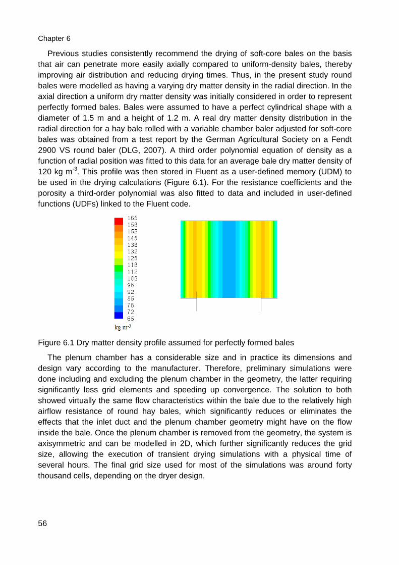
Chapter 6

56

Previous studies consistently recommend the drying of softthat air can penetrate more easily axially compared to uniformimproving air distribution and redubales were modelled as having a varying dry matter density in the radial direction. In the axial direction a uniform dry matter density was initially considered in order to represent perfectly formed bales. Bales were assumed to have a perfect cylindrical shape with a diameter of 1.5 m and a height of 1.2 m. A real dry matter density distribution in the radial direction for a hay bale rolled with a variable chamber baler adjusted for softbales was obtained from a test report by the German Agricultural Society2900 VS round baler (DLG, 2007)function of radial position was fitted to this data for an average bale dry matter density of 120 kg m-3. This profile was then stored in Fluent as a userbe used in the drying calculations (porosity a third-order polynomial was also fitted to data and included in userfunctions (UDFs) linked to the Fluent code.

Figure 6.1 Dry matter density profile assumed for perfectly formed bales

The plenum chamber has a considerable size and in practice its dimensions and design vary according to the manufacturer. Therefore, preliminary simulations were done including and excluding thesignificantly less grid elements and speeding up convergence. The solution to both showed virtually the same flow characteristics within the bale due to the relatively high airflow resistance of round heffects that the inlet duct and the plenum chamber geometry might have on the flow inside the bale. Once the plenum chamber is removed from the geometry, the system is axisymmetric and can be modelledsize, allowing the execution of transient drying simulations with a physical time of several hours. The final grid size used for most of the simulations was around forty thousand cells, depending on the

Previous studies consistently recommend the drying of soft-core bales on the basis that air can penetrate more easily axially compared to uniform-density bales, thereby improving air distribution and reducing drying times. Thus, in the present study round bales were modelled as having a varying dry matter density in the radial direction. In the axial direction a uniform dry matter density was initially considered in order to represent

s. Bales were assumed to have a perfect cylindrical shape with a diameter of 1.5 m and a height of 1.2 m. A real dry matter density distribution in the radial direction for a hay bale rolled with a variable chamber baler adjusted for soft

tained from a test report by the German Agricultural Society(DLG, 2007). A third order polynomial equation of density as a

function of radial position was fitted to this data for an average bale dry matter density of . This profile was then stored in Fluent as a user-defined memory (UDM) to

used in the drying calculations (Figure 6.1). For the resistance coefficients andorder polynomial was also fitted to data and included in user

functions (UDFs) linked to the Fluent code.

Dry matter density profile assumed for perfectly formed bales

The plenum chamber has a considerable size and in practice its dimensions and design vary according to the manufacturer. Therefore, preliminary simulations were done including and excluding the plenum chamber in the geometry, the latter requiring significantly less grid elements and speeding up convergence. The solution to both showed virtually the same flow characteristics within the bale due to the relatively high airflow resistance of round hay bales, which significantly reduces or eliminates the effects that the inlet duct and the plenum chamber geometry might have on the flow inside the bale. Once the plenum chamber is removed from the geometry, the system is axisymmetric and can be modelled in 2D, which further significantly reduces the grid size, allowing the execution of transient drying simulations with a physical time of several hours. The final grid size used for most of the simulations was around forty thousand cells, depending on the dryer design.

core bales on the basis density bales, thereby

cing drying times. Thus, in the present study round bales were modelled as having a varying dry matter density in the radial direction. In the axial direction a uniform dry matter density was initially considered in order to represent

s. Bales were assumed to have a perfect cylindrical shape with a diameter of 1.5 m and a height of 1.2 m. A real dry matter density distribution in the radial direction for a hay bale rolled with a variable chamber baler adjusted for soft-core

tained from a test report by the German Agricultural Society on a Fendt A third order polynomial equation of density as a

function of radial position was fitted to this data for an average bale dry matter density of defined memory (UDM) to

For the resistance coefficients and the order polynomial was also fitted to data and included in user-defined

Dry matter density profile assumed for perfectly formed bales

The plenum chamber has a considerable size and in practice its dimensions and design vary according to the manufacturer. Therefore, preliminary simulations were

plenum chamber in the geometry, the latter requiring significantly less grid elements and speeding up convergence. The solution to both showed virtually the same flow characteristics within the bale due to the relatively high

ay bales, which significantly reduces or eliminates the effects that the inlet duct and the plenum chamber geometry might have on the flow inside the bale. Once the plenum chamber is removed from the geometry, the system is

in 2D, which further significantly reduces the grid size, allowing the execution of transient drying simulations with a physical time of several hours. The final grid size used for most of the simulations was around forty

Chapter 6

57

6.2.1.2 Drying simulation

The simulation of the drying process in a porous media in Fluent requires the coupling of the CFD model with an external drying model. Thorpe (2008) detailed a model to simulate the heat and mass transfer in stored grains, specifically developed to be implemented in CFD software. By changing the product properties and the initial and boundary conditions, it can be used to simulate the drying, cooling or heating of bulks of other agricultural products. It consisted of four UDFs: initialisation, updating of the product moisture content, moisture source and energy source. The model required the drying constant k of the product (Menzies & O’Callaghan, 1971), a sorption isotherm equation (Lamond & Graham, 1993) and additional product parameters (Table 6.1). The humidity of the air was treated as a user-defined scalar (UDS) which was transported in the system. The moisture content of each cell in the bale was stored as a UDM. According to the initial moisture content and temperature of the product defined by the user, the initialisation UDF calculates the humidity ratio in the interstitial air of the product bulk. In the inlet boundary condition the user specified the air velocity, air temperature and moisture ratio. As the air flows through the bale, the program calculated the amount of water lost by the product in each cell and in each time step using the following equations:

%R = −P�� *�*2 6.2

*�*2 = −1(� − ��) 6.3

where W is the product moisture content in the cell and We is the equilibrium moisture content in the cell, both at the current time, and k is a drying constant. The term Sw is the moisture source, whose sign depends on whether moisture is lost or gained by the product. In the case of drying Sw is positive and added to the moisture in the air (the UDS) flowing through the cell. The energy source term is

%M = ℎTP�� *�*2 = −ℎT%R 6.4

where hs is the heat of sorption of water in the product. This energy source term is thus proportional to the moisture source term and in the case of drying is negative, decreasing the temperature of the air flowing through the cell. At the beginning of each time step the moisture content of each cell in the bale was updated.

Although for the drying experiments alfalfa hay was the available product, drying simulations were performed for grass hay due to the data availability in the literature. Table 6.1 summarises the simulation characteristics, settings and properties used.

Chapter 6

58

Table 6.1 Simulation characteristics and settings

Geometry and grid

Bale height 1.2 m

Bale diameter 1.5 m Grid type 2D, quadrilateral, structured Aprox. grid size 40000 cells Cell zone and boundary conditions

Inlet Velocity inlet, normal to boundary, uniform velocity magnitude depending on dryer design corresponding to an airflow of 0.5m3 s-1, air temperature of 38 °C and air humidity ratio of 0.01 kg kg-1

Outlet Pressure outlet Bale Porous media model, anisotropic,

resistance coefficients calculated from VanDuyne & Kjelgaard, 1964 for an average dry matter density of 120 kg m-3. Porosity calculated as a function of bulk density.

Settings Flow conditions Axisymmetric flow, unsteady Air properties Density: incompressible ideal gas law

Viscosity: 1.909 x 10-5 kg m-1 s-1

Specific heat: 1006 J kg-1 K-1 Thermal conductivity: kinetic theory UDS diffusivity: 5.7318 x 10-6 (Thorpe, 2008)

Porous solid properties

Density: 1322 kg m-3 (Williams, 1994) Specific heat: 2290 J kg-1 K-1

(Buckmaster et al., 1989) Thermal conductivity: 0.13 W m-1 K-1

(estimated from results by Opoku et al.(2006)

Turbulence model

k-ε realizable

Discretization Time step size

Second-order upwind Max. 1 s

The air flow and drying in four dryer designs were simulated:

1. Air flows into the lower bale end through an opening 1 m in diameter. The opening has a ring 0.1 m high which pierces the bale. The upper bale end is closed to force the air out through its lateral surface.

2. As in the first design but with a barrier around the lower 0.5 m of the bale lateral surface.

3. The bale has an axial void with a diameter of 0.15 or 0.2 m. The upper bale end is closed.

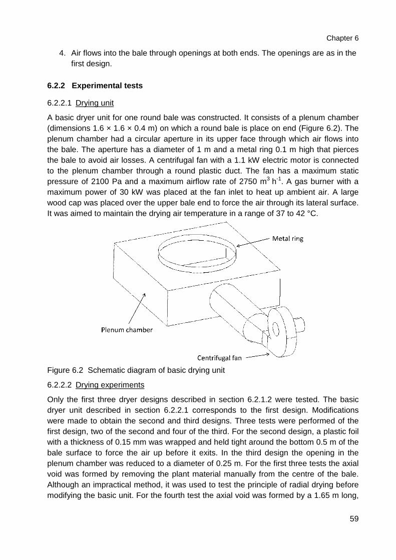
Chapter 6

59

4. Air flows into the bale through openings at both ends. The openings are as in the first design.

6.2.2 Experimental tests

6.2.2.1 Drying unit

A basic dryer unit for one round bale was constructed. It consists of a plenum chamber (dimensions 1.6 × 1.6 × 0.4 m) on which a round bale is place on end (Figure 6.2). The plenum chamber had a circular aperture in its upper face through which air flows into the bale. The aperture has a diameter of 1 m and a metal ring 0.1 m high that pierces the bale to avoid air losses. A centrifugal fan with a 1.1 kW electric motor is connected to the plenum chamber through a round plastic duct. The fan has a maximum static pressure of 2100 Pa and a maximum airflow rate of 2750 m3 h-1. A gas burner with a maximum power of 30 kW was placed at the fan inlet to heat up ambient air. A large wood cap was placed over the upper bale end to force the air through its lateral surface. It was aimed to maintain the drying air temperature in a range of 37 to 42 °C.

Figure 6.2 Schematic diagram of basic drying unit

6.2.2.2 Drying experiments

Only the first three dryer designs described in section 6.2.1.2 were tested. The basic dryer unit described in section 6.2.2.1 corresponds to the first design. Modifications were made to obtain the second and third designs. Three tests were performed of the first design, two of the second and four of the third. For the second design, a plastic foil with a thickness of 0.15 mm was wrapped and held tight around the bottom 0.5 m of the bale surface to force the air up before it exits. In the third design the opening in the plenum chamber was reduced to a diameter of 0.25 m. For the first three tests the axial void was formed by removing the plant material manually from the centre of the bale. Although an impractical method, it was used to test the principle of radial drying before modifying the basic unit. For the fourth test the axial void was formed by a 1.65 m long,

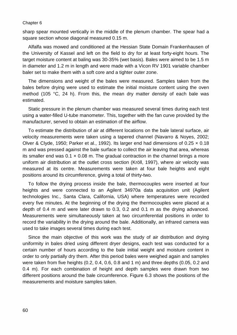
Chapter 6

60

sharp spear mounted vertically in the middle of the plenum chamber. The spear had a square section whose diagonal measured 0.15 m.

Alfalfa was mowed and conditioned at the Hessian State Domain Frankenhausen of the University of Kassel and left on the field to dry for at least forty-eight hours. The target moisture content at baling was 30-35% (wet basis). Bales were aimed to be 1.5 m in diameter and 1.2 m in length and were made with a Vicon RV 1901 variable chamber baler set to make them with a soft core and a tighter outer zone.

The dimensions and weight of the bales were measured. Samples taken from the bales before drying were used to estimate the initial moisture content using the oven method (105 °C, 24 h). From this, the mean dry matter density of each bale was estimated.

Static pressure in the plenum chamber was measured several times during each test using a water-filled U-tube manometer. This, together with the fan curve provided by the manufacturer, served to obtain an estimation of the airflow.

To estimate the distribution of air at different locations on the bale lateral surface, air velocity measurements were taken using a tapered channel (Navarro & Noyes, 2002; Olver & Clyde, 1950; Parker et al., 1992). Its larger end had dimensions of 0.25 × 0.18 m and was pressed against the bale surface to collect the air leaving that area, whereas its smaller end was 0.1 × 0.08 m. The gradual contraction in the channel brings a more uniform air distribution at the outlet cross section (Kröll, 1997), where air velocity was measured at its centre. Measurements were taken at four bale heights and eight positions around its circumference, giving a total of thirty-two.

To follow the drying process inside the bale, thermocouples were inserted at four heights and were connected to an Agilent 34970a data acquisition unit (Agilent technologies Inc., Santa Clara, California, USA) where temperatures were recorded every five minutes. At the beginning of the drying the thermocouples were placed at a depth of 0.4 m and were later drawn to 0.3, 0.2 and 0.1 m as the drying advanced. Measurements were simultaneously taken at two circumferential positions in order to record the variability in the drying around the bale. Additionally, an infrared camera was used to take images several times during each test.

Since the main objective of this work was the study of air distribution and drying uniformity in bales dried using different dryer designs, each test was conducted for a certain number of hours according to the bale initial weight and moisture content in order to only partially dry them. After this period bales were weighed again and samples were taken from five heights (0.2, 0.4, 0.6, 0.8 and 1 m) and three depths (0.05, 0.2 and 0.4 m). For each combination of height and depth samples were drawn from two different positions around the bale circumference. Figure 6.3 shows the positions of the measurements and moisture samples taken.

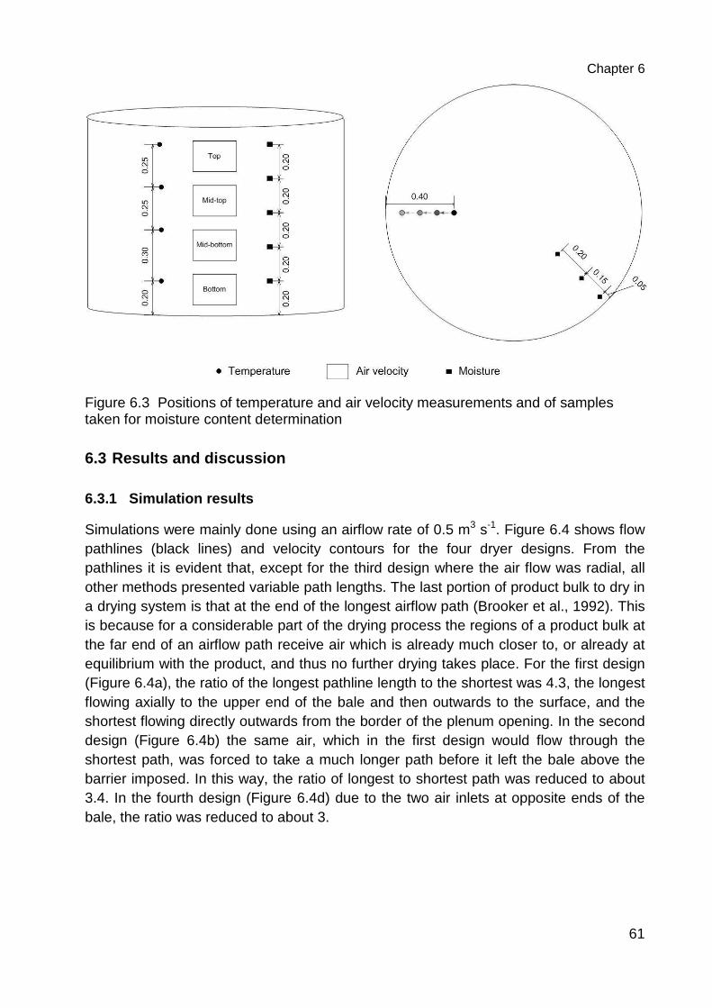
Chapter 6

61

Figure 6.3 Positions of temperature and air velocity measurements and of samples taken for moisture content determination

6.3 Results and discussion

6.3.1 Simulation results

Simulations were mainly done using an airflow rate of 0.5 m3 s-1. Figure 6.4 shows flow pathlines (black lines) and velocity contours for the four dryer designs. From the pathlines it is evident that, except for the third design where the air flow was radial, all other methods presented variable path lengths. The last portion of product bulk to dry in a drying system is that at the end of the longest airflow path (Brooker et al., 1992). This is because for a considerable part of the drying process the regions of a product bulk at the far end of an airflow path receive air which is already much closer to, or already at equilibrium with the product, and thus no further drying takes place. For the first design (Figure 6.4a), the ratio of the longest pathline length to the shortest was 4.3, the longest flowing axially to the upper end of the bale and then outwards to the surface, and the shortest flowing directly outwards from the border of the plenum opening. In the second design (Figure 6.4b) the same air, which in the first design would flow through the shortest path, was forced to take a much longer path before it left the bale above the barrier imposed. In this way, the ratio of longest to shortest path was reduced to about 3.4. In the fourth design (Figure 6.4d) due to the two air inlets at opposite ends of the bale, the ratio was reduced to about 3.

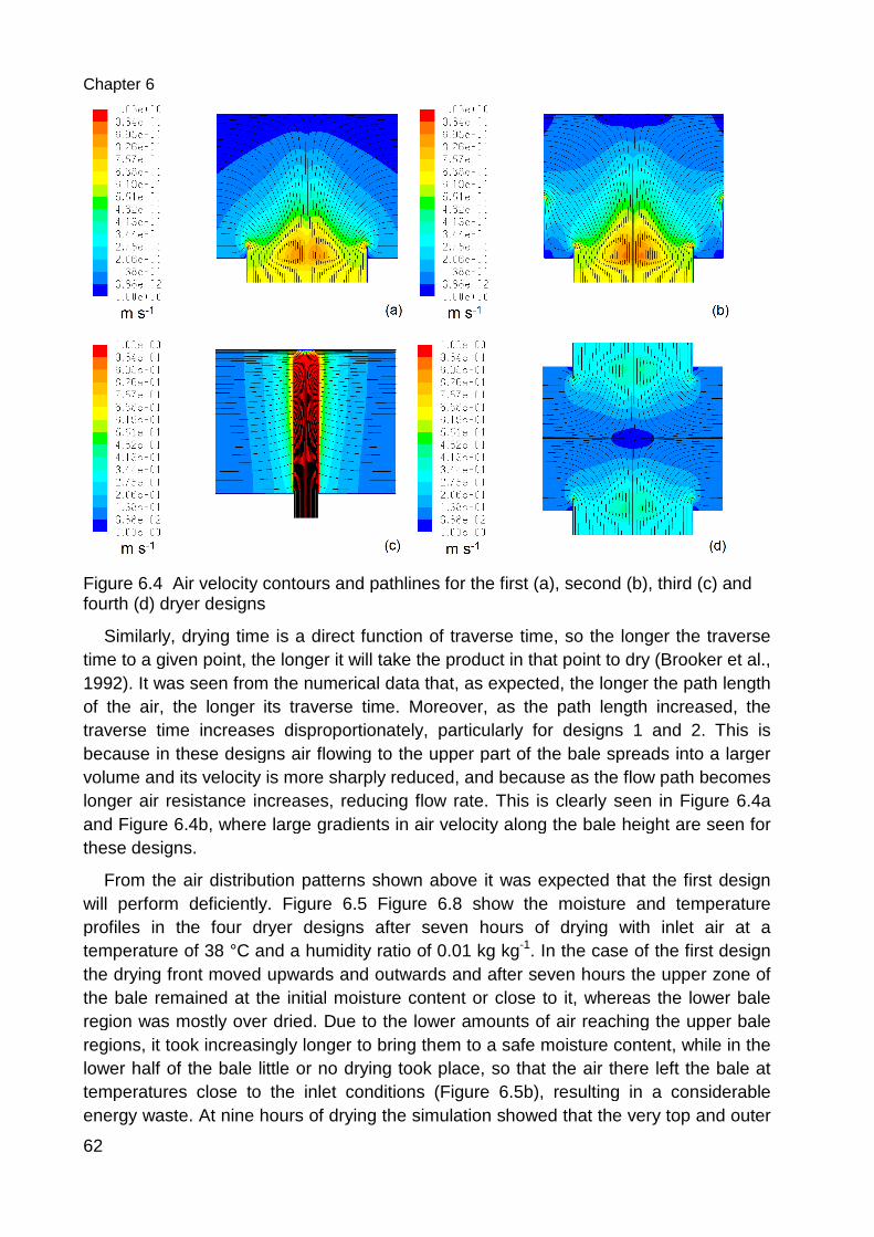
Chapter 6

62

Figure 6.4 Air velocity contours and pathlines for the first (a), second (b), third (c) and fourth (d) dryer designs

Similarly, drying time is a direct function of traverse time, so the longer the traverse time to a given point, the longer it will take the product 1992). It was seen from the numerical data that, as expected, the longer the path length of the air, the longer its traverse time. Moreover, as the path length increased, the traverse time increases disproportionately, particularly fobecause in these designs air flowing to the upper part of the bale spreads into a larger volume and its velocity is more sharply reduced, and because as the flow path becomes longer air resistance increases, reducing flow rate. and Figure 6.4b, where large gradients in air velocity along the bale height are these designs.

From the air distribution patterns shownwill perform deficiently. Figure profiles in the four dryer designs after seven hours temperature of 38 °C and a humidity ratio of 0.01 kg kgthe drying front moved upwards and outwards and after seven hours the upper zone of the bale remained at the initial moisture content oregion was mostly over dried. Due to the lower amounts of air reaching the upper bale regions, it took increasingly longer to bring them to a safe moisture content, while in the lower half of the bale little or no dryitemperatures close to the inlet conditions energy waste. At nine hours of drying the simulation showed that the very top and outer

Air velocity contours and pathlines for the first (a), second (b), third (c) and

Similarly, drying time is a direct function of traverse time, so the longer the traverse time to a given point, the longer it will take the product in that point to dry

It was seen from the numerical data that, as expected, the longer the path length of the air, the longer its traverse time. Moreover, as the path length increased, the traverse time increases disproportionately, particularly for designs 1 and 2. This is because in these designs air flowing to the upper part of the bale spreads into a larger volume and its velocity is more sharply reduced, and because as the flow path becomes longer air resistance increases, reducing flow rate. This is clearly seen in

b, where large gradients in air velocity along the bale height are

patterns shown above it was expected that the first design Figure 6.5 Figure 6.8 show the moisture and temperature

profiles in the four dryer designs after seven hours of drying with inlet air at a temperature of 38 °C and a humidity ratio of 0.01 kg kg-1. In the case of the first design the drying front moved upwards and outwards and after seven hours the upper zone of the bale remained at the initial moisture content or close to it, whereas the lower bale region was mostly over dried. Due to the lower amounts of air reaching the upper bale regions, it took increasingly longer to bring them to a safe moisture content, while in the lower half of the bale little or no drying took place, so that the air there left the bale at temperatures close to the inlet conditions (Figure 6.5b), resulting in a considerable energy waste. At nine hours of drying the simulation showed that the very top and outer

Air velocity contours and pathlines for the first (a), second (b), third (c) and

Similarly, drying time is a direct function of traverse time, so the longer the traverse in that point to dry (Brooker et al.,

It was seen from the numerical data that, as expected, the longer the path length of the air, the longer its traverse time. Moreover, as the path length increased, the

r designs 1 and 2. This is because in these designs air flowing to the upper part of the bale spreads into a larger volume and its velocity is more sharply reduced, and because as the flow path becomes

his is clearly seen in Figure 6.4a b, where large gradients in air velocity along the bale height are seen for

expected that the first design show the moisture and temperature

of drying with inlet air at a In the case of the first design

the drying front moved upwards and outwards and after seven hours the upper zone of r close to it, whereas the lower bale

region was mostly over dried. Due to the lower amounts of air reaching the upper bale regions, it took increasingly longer to bring them to a safe moisture content, while in the

ng took place, so that the air there left the bale at resulting in a considerable

energy waste. At nine hours of drying the simulation showed that the very top and outer

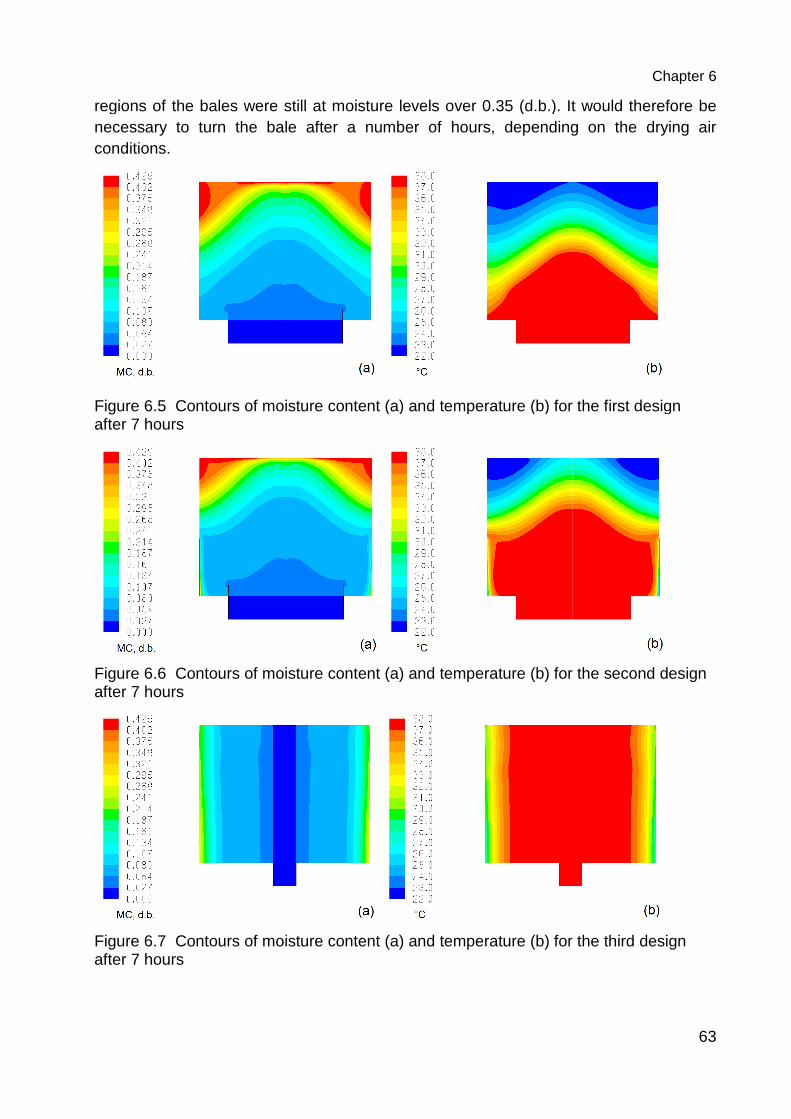
regions of the bales were still at moisture levels over 0.35 (d.b.). It would therefore be necessary to turn the bale after a number of hourconditions.

Figure 6.5 Contours of moisture content (a) and temperature (b) for the first design after 7 hours

Figure 6.6 Contours of moisture content (a) and temperature (b) for the second design after 7 hours

Figure 6.7 Contours of moisture content (a) and temperature (b) for the third design after 7 hours

regions of the bales were still at moisture levels over 0.35 (d.b.). It would therefore be necessary to turn the bale after a number of hours, depending on the drying air

Contours of moisture content (a) and temperature (b) for the first design

Contours of moisture content (a) and temperature (b) for the second design

Contours of moisture content (a) and temperature (b) for the third design

Chapter 6

63

regions of the bales were still at moisture levels over 0.35 (d.b.). It would therefore be s, depending on the drying air

Contours of moisture content (a) and temperature (b) for the first design

Contours of moisture content (a) and temperature (b) for the second design

Contours of moisture content (a) and temperature (b) for the third design

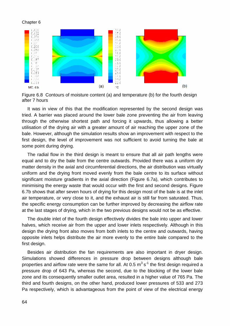
Chapter 6

64

Figure 6.8 Contours of moisture content (a) and temperature (b) for the fourth design after 7 hours

It was in view of this that the modification represented by the second design was tried. A barrier was placed aroundthrough the otherwise shortest path and forcing it upwards, thus allowing a better utilisation of the drying air with a greater amount of air reaching the upper zone of the bale. However, although the sifirst design, the level of improvement was not sufficient to avoid turning the bale at some point during drying.

The radial flow in the third design is meant to ensure that all air path lengths were equal and to dry the bale from the centre outwards. Provided there was a uniform dry matter density in the axial and circumferential directions, the air distribution was virtually uniform and the drying front moved evenly from the bale centre to its surfacsignificant moisture gradients in the axial directionminimising the energy waste that would occur with the first and second designs6.7b shows that after seven hours of drying for this design most of the bale is at the inlet air temperature, or very close to it, and the exhaust air is still far from saturated. Thus, the specific energy consumption can be further improved by decrat the last stages of drying, which in the two previous designs would not be as effective.

The double inlet of the fourth design effectively divides the bale into upper and lower halves, which receive air from the upper and lower indesign the drying front also moves from both inlets to the centre and outwards, having opposite inlets helps distribute the air more evenly to the entire bale compared to the first design.

Besides air distribution the faSimulations showed differences in pressure drop between designs although bale properties and airflow rate were the same for all. At 0.5 mpressure drop of 643 Pa, whereas tzone and its consequently smaller outlet area, resulted in a higher value of 765 Pa. The third and fourth designs, on the other hand, produced lower pressures of 533 and 273 Pa respectively, which is advanta

Contours of moisture content (a) and temperature (b) for the fourth design

It was in view of this that the modification represented by the second design was tried. A barrier was placed around the lower bale zone preventing the air from leaving through the otherwise shortest path and forcing it upwards, thus allowing a better utilisation of the drying air with a greater amount of air reaching the upper zone of the bale. However, although the simulation results show an improvement with respect to the first design, the level of improvement was not sufficient to avoid turning the bale at

The radial flow in the third design is meant to ensure that all air path lengths were equal and to dry the bale from the centre outwards. Provided there was a uniform dry matter density in the axial and circumferential directions, the air distribution was virtually uniform and the drying front moved evenly from the bale centre to its surfacsignificant moisture gradients in the axial direction (Figure 6.7a), which contributes to minimising the energy waste that would occur with the first and second designs

shows that after seven hours of drying for this design most of the bale is at the inlet air temperature, or very close to it, and the exhaust air is still far from saturated. Thus, the specific energy consumption can be further improved by decreasing the airflow rate at the last stages of drying, which in the two previous designs would not be as effective.

The double inlet of the fourth design effectively divides the bale into upper and lower halves, which receive air from the upper and lower inlets respectively. Although in this design the drying front also moves from both inlets to the centre and outwards, having opposite inlets helps distribute the air more evenly to the entire bale compared to the

Besides air distribution the fan requirements are also important in dryer design. Simulations showed differences in pressure drop between designs although bale properties and airflow rate were the same for all. At 0.5 m3 s-1 the first design required a pressure drop of 643 Pa, whereas the second, due to the blocking of the lower bale zone and its consequently smaller outlet area, resulted in a higher value of 765 Pa. The third and fourth designs, on the other hand, produced lower pressures of 533 and 273 Pa respectively, which is advantageous from the point of view of the electrical energy

Contours of moisture content (a) and temperature (b) for the fourth design

It was in view of this that the modification represented by the second design was the lower bale zone preventing the air from leaving

through the otherwise shortest path and forcing it upwards, thus allowing a better utilisation of the drying air with a greater amount of air reaching the upper zone of the

mulation results show an improvement with respect to the first design, the level of improvement was not sufficient to avoid turning the bale at

The radial flow in the third design is meant to ensure that all air path lengths were equal and to dry the bale from the centre outwards. Provided there was a uniform dry matter density in the axial and circumferential directions, the air distribution was virtually uniform and the drying front moved evenly from the bale centre to its surface without

which contributes to minimising the energy waste that would occur with the first and second designs. Figure

shows that after seven hours of drying for this design most of the bale is at the inlet air temperature, or very close to it, and the exhaust air is still far from saturated. Thus,

easing the airflow rate at the last stages of drying, which in the two previous designs would not be as effective.

The double inlet of the fourth design effectively divides the bale into upper and lower lets respectively. Although in this

design the drying front also moves from both inlets to the centre and outwards, having opposite inlets helps distribute the air more evenly to the entire bale compared to the

n requirements are also important in dryer design. Simulations showed differences in pressure drop between designs although bale

the first design required a he second, due to the blocking of the lower bale

zone and its consequently smaller outlet area, resulted in a higher value of 765 Pa. The third and fourth designs, on the other hand, produced lower pressures of 533 and 273

geous from the point of view of the electrical energy

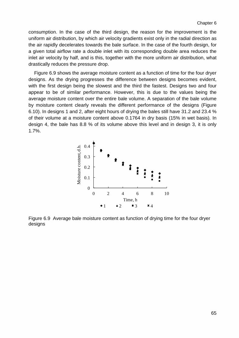
Chapter 6

65

consumption. In the case of the third design, the reason for the improvement is the uniform air distribution, by which air velocity gradients exist only in the radial direction as the air rapidly decelerates towards the bale surface. In the case of the fourth design, for a given total airflow rate a double inlet with its corresponding double area reduces the inlet air velocity by half, and is this, together with the more uniform air distribution, what drastically reduces the pressure drop.

Figure 6.9 shows the average moisture content as a function of time for the four dryer designs. As the drying progresses the difference between designs becomes evident, with the first design being the slowest and the third the fastest. Designs two and four appear to be of similar performance. However, this is due to the values being the average moisture content over the entire bale volume. A separation of the bale volume by moisture content clearly reveals the different performance of the designs (Figure 6.10). In designs 1 and 2, after eight hours of drying the bales still have 31.2 and 23.4 % of their volume at a moisture content above 0.1764 in dry basis (15% in wet basis). In design 4, the bale has 8.8 % of its volume above this level and in design 3, it is only 1.7%.

Figure 6.9 Average bale moisture content as function of drying time for the four dryer designs

0

0.1

0.2

0.3

0.4

0 2 4 6 8 10

Mo

istu

re c

on

ten

t, d

.b.

Time, h1 2 3 4

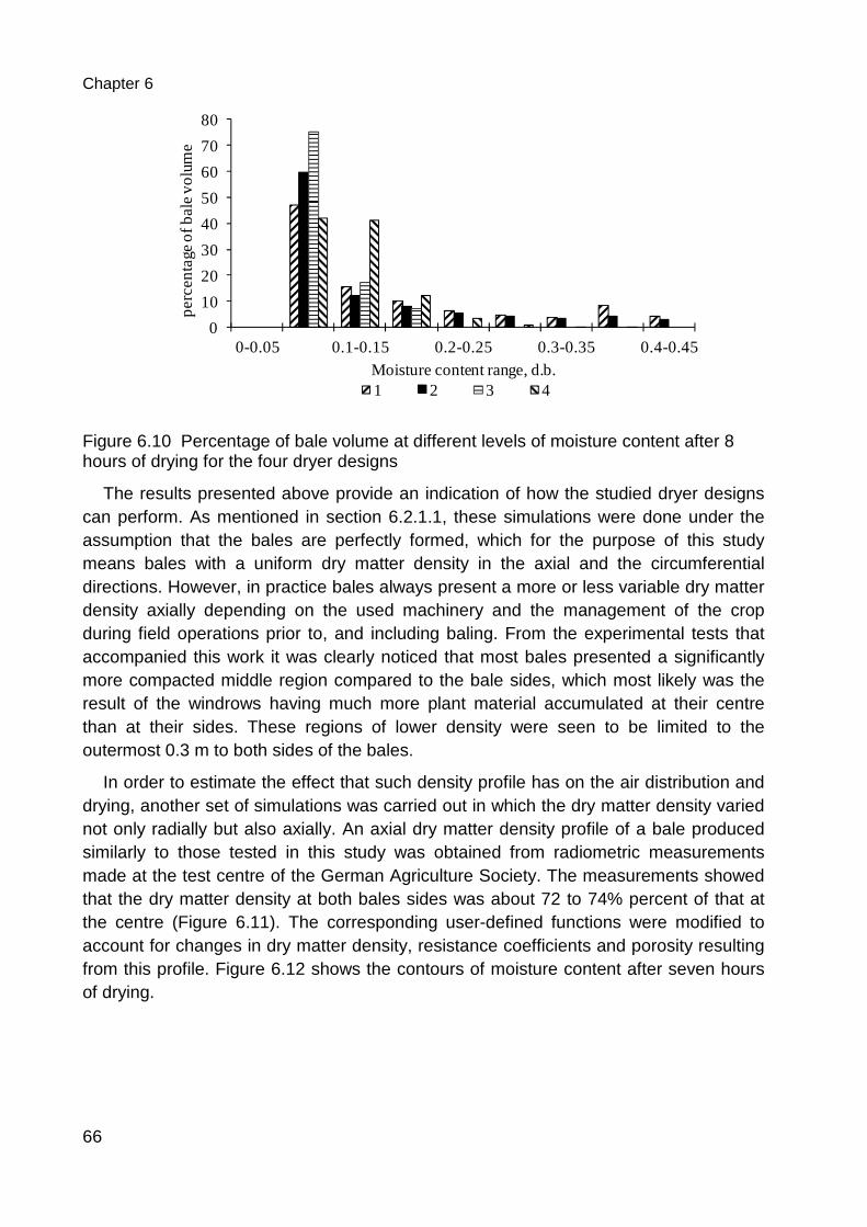
Chapter 6

66

Figure 6.10 Percentage of bale volume at different levels of moisture content after 8 hours of drying for the four dryer designs

The results presented above provide an indication of how the studied dryer designs can perform. As mentioned in section 6.2.1.1, these simulations were done under the assumption that the bales are perfectly formed, which for the purpose of this study means bales with a uniform dry matter density in the axial and the circumferential directions. However, in practice bales always present a more or less variable dry matter density axially depending on the used machinery and the management of the crop during field operations prior to, and including baling. From the experimental tests that accompanied this work it was clearly noticed that most bales presented a significantly more compacted middle region compared to the bale sides, which most likely was the result of the windrows having much more plant material accumulated at their centre than at their sides. These regions of lower density were seen to be limited to the outermost 0.3 m to both sides of the bales.

In order to estimate the effect that such density profile has on the air distribution and drying, another set of simulations was carried out in which the dry matter density varied not only radially but also axially. An axial dry matter density profile of a bale produced similarly to those tested in this study was obtained from radiometric measurements made at the test centre of the German Agriculture Society. The measurements showed that the dry matter density at both bales sides was about 72 to 74% percent of that at the centre (Figure 6.11). The corresponding user-defined functions were modified to account for changes in dry matter density, resistance coefficients and porosity resulting from this profile. Figure 6.12 shows the contours of moisture content after seven hours of drying.

0

10

20

30

40

50

60

70

80

0-0.05 0.1-0.15 0.2-0.25 0.3-0.35 0.4-0.45

pe

rce

nta

ge o

f ba

le v

olu

me

Moisture content range, d.b.1 2 3 4

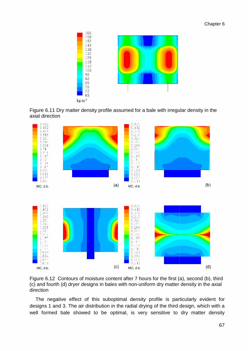
Figure 6.11 Dry matter density profile assumed foraxial direction

Figure 6.12 Contours of moisture content after 7 hours for the first (a), second (b), third (c) and fourth (d) dryer designs in bales with nondirection

The negative effect of this suboptimal density profile is particularly evdesigns 1 and 3. The air distribution in the radial drying of the third design, which with a well formed bale showed to be optimal, is very sensitive to dry matter density

ry matter density profile assumed for a bale with irregular density in the

Contours of moisture content after 7 hours for the first (a), second (b), third (c) and fourth (d) dryer designs in bales with non-uniform dry matter density in the axial

The negative effect of this suboptimal density profile is particularly evdesigns 1 and 3. The air distribution in the radial drying of the third design, which with a well formed bale showed to be optimal, is very sensitive to dry matter density

Chapter 6

67

a bale with irregular density in the

Contours of moisture content after 7 hours for the first (a), second (b), third uniform dry matter density in the axial

The negative effect of this suboptimal density profile is particularly evident for designs 1 and 3. The air distribution in the radial drying of the third design, which with a well formed bale showed to be optimal, is very sensitive to dry matter density

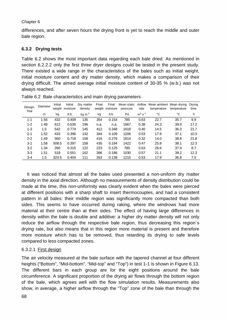
Chapter 6

68

differences, and after seven hours the drying front is yet to reach the middle and outer bale region.

6.3.2 Drying tests

Table 6.2 shows the most important data regarding each bale dried. As mentioned in section 6.2.2.2 only the first three dryer designs could be tested in the present study. There existed a wide range in the characteristics of the bales such as initial weight, initial moisture content and dry matter density, which makes a comparison of their drying difficult. The aimed average initial moisture content of 30-35 % (w.b.) was not always reached.

Table 6.2 Bale characteristics and main drying parameters

It was noticed that almost all the bales used presented a non-uniform dry matter density in the axial direction. Although no measurements of density distribution could be made at the time, this non-uniformity was clearly evident when the bales were pierced at different positions with a sharp shaft to insert thermocouples, and had a consistent pattern in all bales: their middle region was significantly more compacted than both sides. This seems to have occurred during raking, where the windrows had more material at their centre than at their sides. The effect of having large differences in density within the bale is double and additive: a higher dry matter density will not only reduce the airflow through the respective bale region, thus decreasing this region´s drying rate, but also means that in this region more material is present and therefore more moisture which has to be removed, thus retarding its drying to safe levels compared to less compacted zones.

6.3.2.1 First design

The air velocity measured at the bale surface with the tapered channel at four different heights (“Bottom”, “Mid-bottom”, “Mid-top” and “Top”) in test 1-1 is shown in Figure 6.13. The different bars in each group are for the eight positions around the bale circumference. A significant proportion of the drying air flows through the bottom region of the bale, which agrees well with the flow simulation results. Measurements also show, in average, a higher airflow through the “Top” zone of the bale than through the

DiameterInitial

weightInitial

moistureDry matter

density Final

weightFinal

moistureMean static

pressureAirflow

rateMean ambient temperature

Mean drying temperature

Drying time

m kg d.b. kg m-3 kg d.b. Pa m3 s-1 °C °C h

1-1 1.56 432 0.409 135 354 0.154 785 0.63 22.7 35.7 9.91-2 1.48 612 0.535 196 n.a. n.a. 1667 0.38 24.3 39.9 17.21-3 1.5 542 0.774 145 412 0.348 1618 0.40 14.5 36.3 21.72-1 1.52 433 0.396 142 344 0.109 1206 0.53 17.9 37.1 10.32-2 1.49 560 0.718 158 416 0.276 1814 0.32 14.0 38.8 21.83-1 1.58 508.5 0.397 158 435 0.194 1422 0.47 25.8 38.1 12.33-2 1.34 260 0.315 122 223 0.125 785 0.63 26.6 37.9 8.73-3 1.51 518 0.551 162 396 0.186 1030 0.57 21.1 39.2 12.33-4 1.5 324.5 0.404 111 263 0.138 1215 0.53 17.9 36.8 7.5

Design-Trial

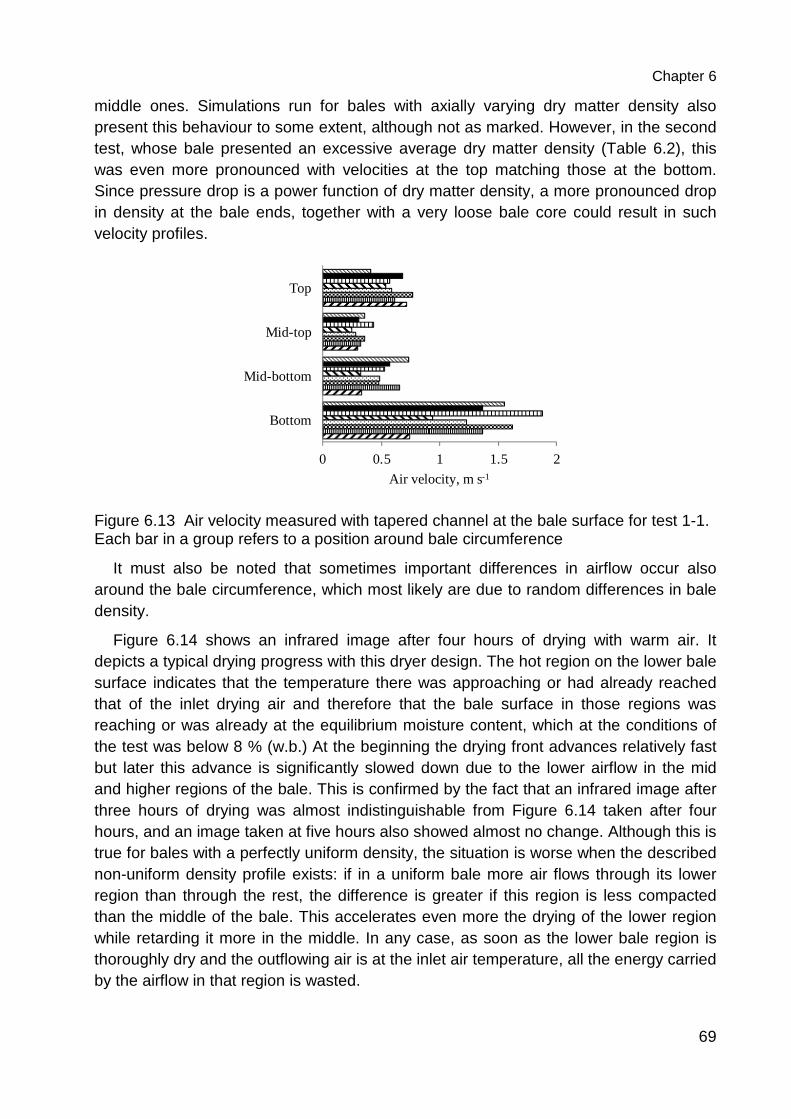
Chapter 6

69

middle ones. Simulations run for bales with axially varying dry matter density also present this behaviour to some extent, although not as marked. However, in the second test, whose bale presented an excessive average dry matter density (Table 6.2), this was even more pronounced with velocities at the top matching those at the bottom. Since pressure drop is a power function of dry matter density, a more pronounced drop in density at the bale ends, together with a very loose bale core could result in such velocity profiles.

Figure 6.13 Air velocity measured with tapered channel at the bale surface for test 1-1. Each bar in a group refers to a position around bale circumference

It must also be noted that sometimes important differences in airflow occur also around the bale circumference, which most likely are due to random differences in bale density.

Figure 6.14 shows an infrared image after four hours of drying with warm air. It depicts a typical drying progress with this dryer design. The hot region on the lower bale surface indicates that the temperature there was approaching or had already reached that of the inlet drying air and therefore that the bale surface in those regions was reaching or was already at the equilibrium moisture content, which at the conditions of the test was below 8 % (w.b.) At the beginning the drying front advances relatively fast but later this advance is significantly slowed down due to the lower airflow in the mid and higher regions of the bale. This is confirmed by the fact that an infrared image after three hours of drying was almost indistinguishable from Figure 6.14 taken after four hours, and an image taken at five hours also showed almost no change. Although this is true for bales with a perfectly uniform density, the situation is worse when the described non-uniform density profile exists: if in a uniform bale more air flows through its lower region than through the rest, the difference is greater if this region is less compacted than the middle of the bale. This accelerates even more the drying of the lower region while retarding it more in the middle. In any case, as soon as the lower bale region is thoroughly dry and the outflowing air is at the inlet air temperature, all the energy carried by the airflow in that region is wasted.

0 0.5 1 1.5 2

Top

Mid-top

Mid-bottom

Bottom

Air velocity, m s-1

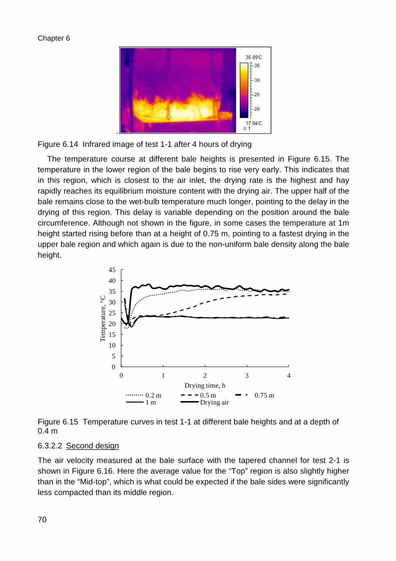
Chapter 6

70

.

Figure 6.14 Infrared image of test 1-1 after 4 hours of drying

The temperature course at different bale heights is presented in Figure 6.15. The temperature in the lower region of the bale begins to rise very early. This indicates that in this region, which is closest to the air inlet, the drying rate is the highest and hay rapidly reaches its equilibrium moisture content with the drying air. The upper half of the bale remains close to the wet-bulb temperature much longer, pointing to the delay in the drying of this region. This delay is variable depending on the position around the bale circumference. Although not shown in the figure, in some cases the temperature at 1m height started rising before than at a height of 0.75 m, pointing to a fastest drying in the upper bale region and which again is due to the non-uniform bale density along the bale height.

Figure 6.15 Temperature curves in test 1-1 at different bale heights and at a depth of 0.4 m

6.3.2.2 Second design

The air velocity measured at the bale surface with the tapered channel for test 2-1 is shown in Figure 6.16. Here the average value for the “Top” region is also slightly higher than in the “Mid-top”, which is what could be expected if the bale sides were significantly less compacted than its middle region.

0

5

10

15

20

25

30

35

40

45

0 1 2 3 4

Tem

pera

ture

, °C

Drying time, h

0.2 m 0.5 m 0.75 m1 m Drying air

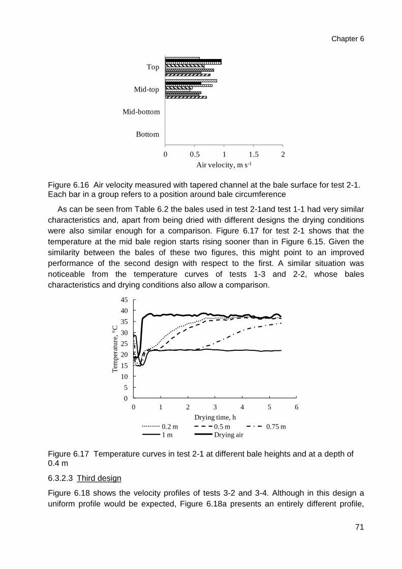
Chapter 6

71

Figure 6.16 Air velocity measured with tapered channel at the bale surface for test 2-1. Each bar in a group refers to a position around bale circumference

As can be seen from Table 6.2 the bales used in test 2-1and test 1-1 had very similar characteristics and, apart from being dried with different designs the drying conditions were also similar enough for a comparison. Figure 6.17 for test 2-1 shows that the temperature at the mid bale region starts rising sooner than in Figure 6.15. Given the similarity between the bales of these two figures, this might point to an improved performance of the second design with respect to the first. A similar situation was noticeable from the temperature curves of tests 1-3 and 2-2, whose bales characteristics and drying conditions also allow a comparison.

Figure 6.17 Temperature curves in test 2-1 at different bale heights and at a depth of 0.4 m

6.3.2.3 Third design

Figure 6.18 shows the velocity profiles of tests 3-2 and 3-4. Although in this design a uniform profile would be expected, Figure 6.18a presents an entirely different profile,

0 0.5 1 1.5 2

Top

Mid-top

Mid-bottom

Bottom

Air velocity, m s-1

0

5

10

15

20

25

30

35

40

45

0 1 2 3 4 5 6

Tem

per

atu

re, °

C

Drying time, h0.2 m 0.5 m 0.75 m1 m Drying air

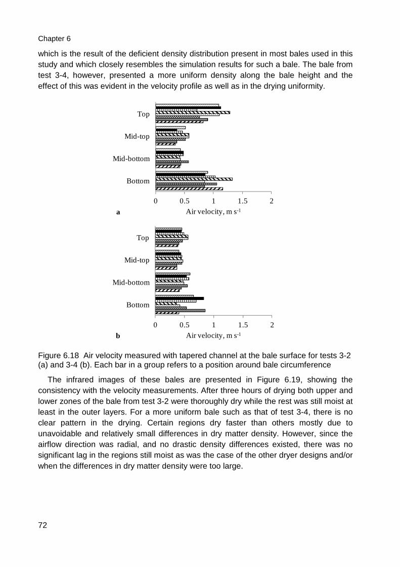
Chapter 6

72

which is the result of the deficient density distribution present in most bales used in this study and which closely resembles the simulation results for such a bale. The bale from test 3-4, however, presented a more uniform density along the bale height and the effect of this was evident in the velocity profile as well as in the drying uniformity.

Figure 6.18 Air velocity measured with tapered channel at the bale surface for tests 3-2 (a) and 3-4 (b). Each bar in a group refers to a position around bale circumference

The infrared images of these bales are presented in Figure 6.19, showing the consistency with the velocity measurements. After three hours of drying both upper and lower zones of the bale from test 3-2 were thoroughly dry while the rest was still moist at least in the outer layers. For a more uniform bale such as that of test 3-4, there is no clear pattern in the drying. Certain regions dry faster than others mostly due to unavoidable and relatively small differences in dry matter density. However, since the airflow direction was radial, and no drastic density differences existed, there was no significant lag in the regions still moist as was the case of the other dryer designs and/or when the differences in dry matter density were too large.

0 0.5 1 1.5 2

Top

Mid-top

Mid-bottom

Bottom

Air velocity, m s-1a

0 0.5 1 1.5 2

Top

Mid-top

Mid-bottom

Bottom

Air velocity, m s-1b

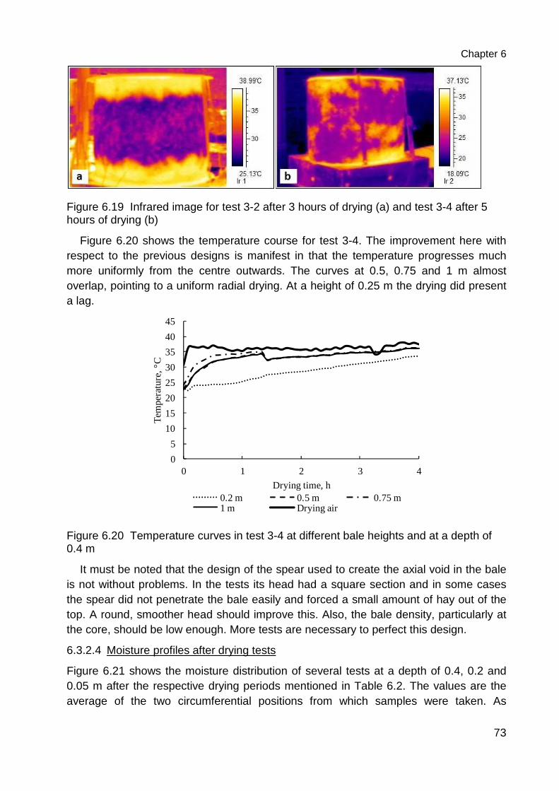
Chapter 6

73

Figure 6.19 Infrared image for test 3-2 after 3 hours of drying (a) and test 3-4 after 5 hours of drying (b)

Figure 6.20 shows the temperature course for test 3-4. The improvement here with respect to the previous designs is manifest in that the temperature progresses much more uniformly from the centre outwards. The curves at 0.5, 0.75 and 1 m almost overlap, pointing to a uniform radial drying. At a height of 0.25 m the drying did present a lag.

Figure 6.20 Temperature curves in test 3-4 at different bale heights and at a depth of 0.4 m

It must be noted that the design of the spear used to create the axial void in the bale is not without problems. In the tests its head had a square section and in some cases the spear did not penetrate the bale easily and forced a small amount of hay out of the top. A round, smoother head should improve this. Also, the bale density, particularly at the core, should be low enough. More tests are necessary to perfect this design.

6.3.2.4 Moisture profiles after drying tests

Figure 6.21 shows the moisture distribution of several tests at a depth of 0.4, 0.2 and 0.05 m after the respective drying periods mentioned in Table 6.2. The values are the average of the two circumferential positions from which samples were taken. As

0

5

10

15

20

25

30

35

40

45

0 1 2 3 4

Tem

pera

ture

, °C

Drying time, h0.2 m 0.5 m 0.75 m1 m Drying air

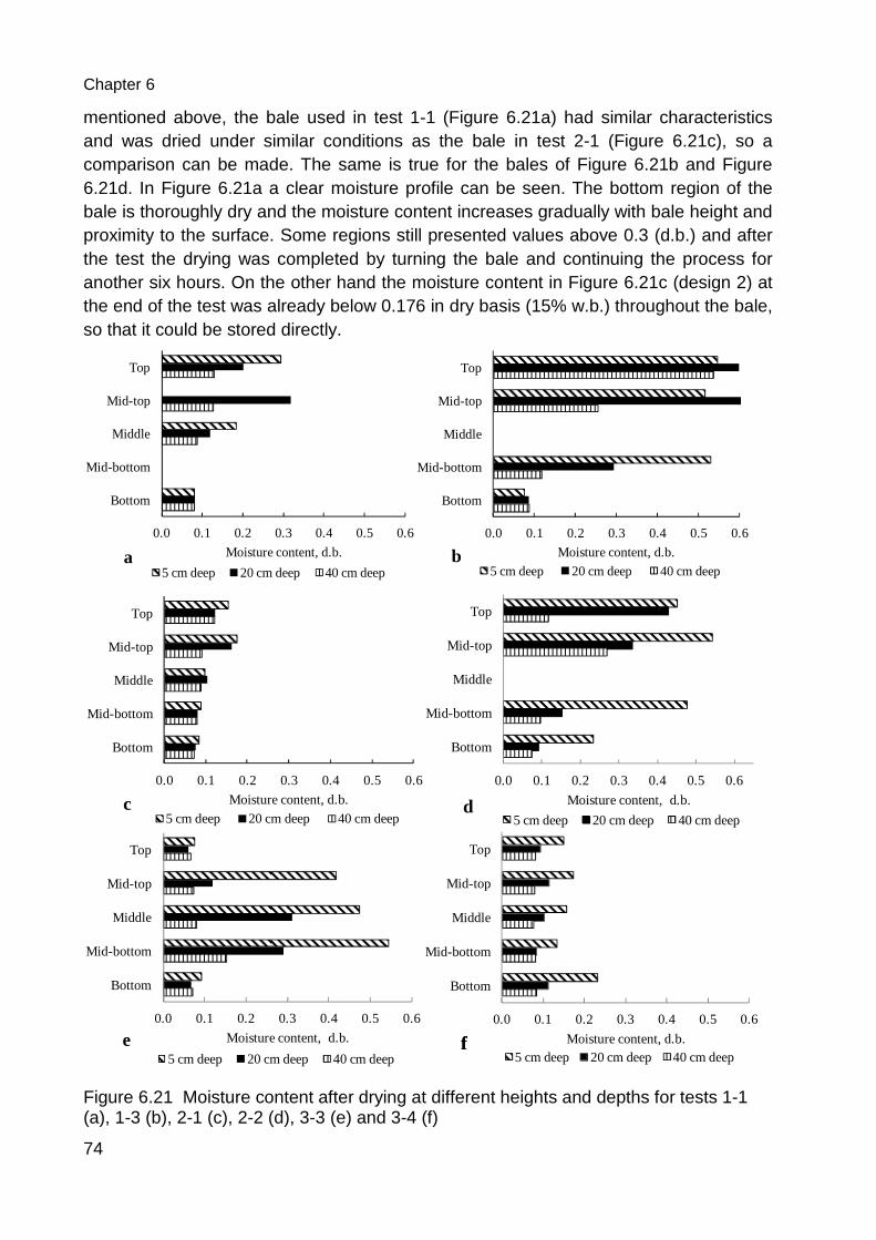
Chapter 6

74

mentioned above, the bale used in test 1-1 (Figure 6.21a) had similar characteristics and was dried under similar conditions as the bale in test 2-1 (Figure 6.21c), so a comparison can be made. The same is true for the bales of Figure 6.21b and Figure 6.21d. In Figure 6.21a a clear moisture profile can be seen. The bottom region of the bale is thoroughly dry and the moisture content increases gradually with bale height and proximity to the surface. Some regions still presented values above 0.3 (d.b.) and after the test the drying was completed by turning the bale and continuing the process for another six hours. On the other hand the moisture content in Figure 6.21c (design 2) at the end of the test was already below 0.176 in dry basis (15% w.b.) throughout the bale, so that it could be stored directly.

Figure 6.21 Moisture content after drying at different heights and depths for tests 1-1 (a), 1-3 (b), 2-1 (c), 2-2 (d), 3-3 (e) and 3-4 (f)

0.0 0.1 0.2 0.3 0.4 0.5 0.6

Top

Mid-top

Middle

Mid-bottom

Bottom

Moisture content, d.b.

5 cm deep 20 cm deep 40 cm deepa

0.0 0.1 0.2 0.3 0.4 0.5 0.6

Top

Mid-top

Middle

Mid-bottom

Bottom

Moisture content, d.b.

5 cm deep 20 cm deep 40 cm deepb

0.0 0.1 0.2 0.3 0.4 0.5 0.6

Top

Mid-top

Middle

Mid-bottom

Bottom

Moisture content, d.b.

5 cm deep 20 cm deep 40 cm deepc

0.0 0.1 0.2 0.3 0.4 0.5 0.6

Top

Mid-top

Middle

Mid-bottom

Bottom

Moisture content, d.b.

5 cm deep 20 cm deep 40 cm deepd

0.0 0.1 0.2 0.3 0.4 0.5 0.6

Top

Mid-top

Middle

Mid-bottom

Bottom

Moisture content, d.b.

5 cm deep 20 cm deep 40 cm deepe

0.0 0.1 0.2 0.3 0.4 0.5 0.6

Top

Mid-top

Middle

Mid-bottom

Bottom

Moisture content, d.b.5 cm deep 20 cm deep 40 cm deep

ff

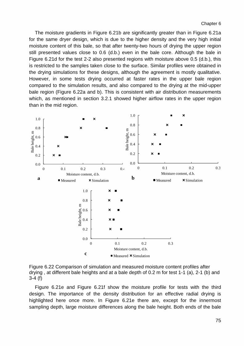
Chapter 6

75

The moisture gradients in Figure 6.21b are significantly greater than in Figure 6.21a for the same dryer design, which is due to the higher density and the very high initial moisture content of this bale, so that after twenty-two hours of drying the upper region still presented values close to 0.6 (d.b.) even in the bale core. Although the bale in Figure 6.21d for the test 2-2 also presented regions with moisture above 0.5 (d.b.), this is restricted to the samples taken close to the surface. Similar profiles were obtained in the drying simulations for these designs, although the agreement is mostly qualitative. However, in some tests drying occurred at faster rates in the upper bale region compared to the simulation results, and also compared to the drying at the mid-upper bale region (Figure 6.22a and b). This is consistent with air distribution measurements which, as mentioned in section 3.2.1 showed higher airflow rates in the upper region than in the mid region.

Figure 6.22 Comparison of simulation and measured moisture content profiles after drying , at different bale heights and at a bale depth of 0.2 m for test 1-1 (a), 2-1 (b) and 3-4 (f)

Figure 6.21e and Figure 6.21f show the moisture profile for tests with the third design. The importance of the density distribution for an effective radial drying is highlighted here once more. In Figure 6.21e there are, except for the innermost sampling depth, large moisture differences along the bale height. Both ends of the bale

0.0

0.2

0.4

0.6

0.8

1.0

0 0.1 0.2 0.3 0.4

Bal

e he

ight

, m

Moisture content, d.b.

Measured Simulationa

0.0

0.2

0.4

0.6

0.8

1.0

0 0.1 0.2 0.3

Bal

e he

igh

t, m

Moisture content, d.b.

Measured Simulationb

0.0

0.2

0.4

0.6

0.8

1.0

0 0.1 0.2 0.3

Bal

e he

ight

, m

Moisture content, d.b.

Measured Simulationc

Chapter 6

76

were thoroughly dry whereas the outer portion in the middle region was still largely under dried, which agrees well with simulation results of Figure 6.12c. Similar results were obtained by Brandemuehl et al. (1988) when bales were rolled from narrow windrows. However when bales were made from wide swaths their result was reversed and it was the middle of the bales which dried faster. In Figure 6.21f, in which the bale had a much more uniform density product of a well formed swath, there were no such large moisture gradients along the bale height and the drying progressed close to what was expected in a radial drying under optimal conditions as shown by the drying simulation (Figure 6.22c). Although not observable from Figure 6.21 moisture gradients also existed along the bale circumference as indicated by the temperature and air velocity measurements.

As mentioned above and shown in Figure 6.22, the experimental moisture profiles are, in general, in good qualitative agreement with simulation results. However, a close quantitative agreement was not possible due to the differences between the real bale and process characteristics, and the assumptions made for simulations.

6.4 Conclusions

Air and moisture distribution in round bales differ significantly among the dryer designs studied. Simple, single inlet dryers produce a deficient air distribution with some bale regions barely receiving airflow. This results in extended drying time and a reduced drying efficiency. When bales were assumed to be perfectly formed, the evaluated modifications, namely imposing a barrier to the lower portion of the bale surface, the formation of a void along the bale axis to create radial flow, and the use of two air inlets at both bale ends, all improved drying to a lesser or greater extent. The third design studied would theoretically be the best choice due to the radial airflow it causes, which produces a radially moving drying front. However, the bale characteristics in terms of uniformity of its dry matter density are important for the successful operation of any dryer. Although the results obtained showed the positive effects of the proposed modifications, the number of tests performed was relatively small. More research in this area is needed, including tests regarding the feasibility of producing well formed, uniform density bales consistently under practical conditions, and the optimisation of the spear used in the third design. In general the experimental results showed a good qualitative agreement with CFD simulations. Infrared images as well as temperature measurements at different positions and depths are useful means for judging the progress and uniformity of the drying process.

77

7 Real-time product moisture content monitoring in batch dryer using psychrometric and airflow measurements

The possibility of a continuous monitoring of moisture content in batch dryers using air humidity was studied in a laboratory-scale test stand. Psychrometers formed by two K-type thermocouples, one of them kept moist, were installed at the system inlet and outlet to measure the increase in the humidity of the drying air. A grid measurement of air velocity at the inlet duct was used to estimate the airflow from a single measurement point. The sensors were connected to a data logger and this to a computer. An algorithm written in MATLAB allowed the retrieval of measured data from the data logger at specified time intervals and the calculation of the mass of water removed. Numerous drying trials have shown that this method can be suitable for drying monitoring. Errors in the calculation of final moisture content of less than 0.03 (dry basis) could be obtained. The difficulty in measuring wet-bulb temperature with sufficient accuracy over long periods was seen as the main obstacle for a reliable use of the method. Attention must be paid to different possible sources of error, which can be minimized by adequate sensor selection and location.

7.1 Introduction

Monitoring the moisture content of a product during drying is a complicated task. For convective batch dryers, the simplest, cheapest and most traditional method is to take a sample and determine its moisture content in an oven at a high temperature. Although this method can be very accurate, it is often of limited use since the results are obtained after some time, in many cases hours, which prevents a real-time monitoring of the process. Also, depending on dryer type, sample extraction might involve stopping the process which during commercial production is not advisable (Briens & Bojarra, 2010). In many cases, particularly but not only in small-scale facilities the moisture content is estimated by experience based on inspection of the product, which is inevitably subjective and inaccurate. There are also electrical methods for the measurement of solids’ moisture content, which are based on the dependence of electrical resistance and dielectric properties of the material on its moisture content (Molnár, 2006). They are fast and in some cases the sensor probes can be introduced into the product bed for continuous monitoring at the measurement point. However they are restricted to a set of products like grain, wood and hay, their accuracy is dependent on many factors and they need to be calibrated for each product.

The methods mentioned above measure the moisture at a particular location in the dryer, and therefore by taking numerous measurements at different positions they are useful to determine the moisture profile resulting from spatially varying drying conditions in the product bulk. However, in many cases it might be useful to know additionally (or only) the average moisture content in the bulk and such methods are in this case less useful. An option to estimate the average moisture content of the bulk is through the

Chapter 7

78

monitoring of the product and/or the outflowing air temperature, since during most of the drying process both are cooled down due to water evaporation. At some point when the water content of the product reaches a critical point, the temperature of outflowing air and product will raise until it reaches the inlet air temperature, thus marking the end of the process. Because the bed temperature only begins to increase once surface moisture is lost from the particles, this type of temperature monitoring only provides information about bed moisture content late in the drying process (Chaplin et al., 2005).

Another possibility, and the one considered in the present study, would be to directly calculate the amount of water evaporated from the product. This can be done by precise and continuous measurement of air humidity before and after it passes through the product as well as of the airflow rate. Although the principle of this method is of course not new, no studies have been found to assess its accuracy and feasibility. Such a method was employed in some studies to follow the drying progress. However, in general the applicability of the method was not the topic of study and no estimation of its accuracy was obtained (Arinze et al., 1996; Godsalve et al., 1977). Correa-Hernando et al. (2011) developed three model-based methods for the supervision of a solar dryer, one of which was based on calculations from inlet and outlet air conditions and airflow rate. However, their results show a large difference between measured and calculated weight loss. Therefore, the objective of this study was to assess the applicability of air humidity and flow measurements to monitor the course of the drying process in batch dryers.

7.2 Materials and methods

7.2.1 Apparatus

An existing apparatus to measure the airflow resistance of bulks of agricultural products was modified and equipped with the necessary sensors. Figure 7.1 shows a schematic diagram. The main parts of the apparatus are inlet duct, butterfly valve, centrifugal in-line duct fan, test column and outlet duct.

The entrance to the apparatus consisted of a round galvanized steel air duct with a diameter of 0.15 m and a length of 0.85 m. At 0.3 m downstream from the duct inlet a honeycomb flow straightener with tube diameter of 0.005 m and tube length of 0.05 m was installed to remove any tangential velocity components. The butterfly valve was installed immediately upstream of the fan in order to reduce the airflow to the desired test conditions. Below the perforated plate which formed the bottom of the test column, three additional perforated plates with a space between them of 0.05 m were installed to improve the flow uniformity after the change of direction in the plenum chamber. The test column had a height and a diameter of 0.6 m.

Chapter 7

79

Figure 7.1 Schematic diagram of test apparatus: inlet duct (a), flow straightener (b), butterfly valve (c), in-line duct fan (d), perforated plates (e), test column (f), outlet duct (g)

An Airflow TA-5 hot wire anemometer with a full scale accuracy of ± 1% (FS of 15 m s-1) in its analogue output was used to measure air velocity. The probe was placed at the duct centre and 0.4 m downstream of the flow straightener. To determine the airflow rate in the system from a single measurement point, the guideline VDI/VDE 2640 Part 3 (1983) was used, which details the procedures to determine the flow rate of gases in ducts of circular, annular and rectangular cross sections by means of grid measurements. For this, the circular cross section of the duct was divided in three concentric surfaces of equal area, and the circular line dividing again each surface in two equal areas (circular dotted lines in Figure 7.2) was determined. Twenty-four measurement points in the centroid of twenty-four equal-area surfaces are thus established by the intersection of these lines and eight radial lines (straight dotted lines in Figure 7.2) distributed around the circumference.

Figure 7.2 Measurement positions for the grid measurement

Chapter 7

80

Since the measurements could only be done successively, and small, slow changes in flow rate cannot be excluded, a reference measurement vr in the duct centre is taken immediately after each point measurement vi. The influence of airflow fluctuation is taken into account by working with the velocity ratio vi/vr. To account for the effect of the duct wall on the velocity profile a correction is introduced. A reference factor is calculated from the measured data as follows: QAQU = Q̅QU − WQ̅(QU − Q̅�QUX 1� 7.1

where v̅/vr is the mean of the velocity ratio over the twenty-four measurement points, v̅1/vr and v̅2/vr are the means of the velocity ratio in the first and second outermost concentric surfaces respectively, and k/n is a correction factor for the duct wall effect. Finally the airflow rate at a given time can be calculated as follows:

YZ(2#) = WQAQU X QU(2#)[ 7.2

where vr(ti) is a velocity measurement at the duct centre and A is the cross-sectional area of the duct.

To form a psychrometer two ungrounded type-K thermocouples with a probe sheath diameter of 3 mm were installed in close proximity to each other and 0.05 m downstream of the anemometer. One of them was kept moist by a cloth wick partly immersed in distilled water. Another such pair of thermocouples was installed in the outlet duct. Before the tests the thermocouples were calibrated in an ice water bath.

The thermocouples and the hot wire anemometer were connected to an Agilent 34970a data acquisition device (DAQ) and this was connected to a computer.

7.2.2 Algorithm

A program was written in MATLAB to communicate with the data acquisition device, retrieve the temperature and air velocity measurements at specified intervals, and perform the calculations to determine the mass of water evaporated. A flowchart of the program appears in Figure 7.3.

To calculate the humidity ratio from the dry and wet-bulb temperatures the following equations (ASHRAE, 2009) are used:

First the saturation vapour pressure of water pws at the wet-bulb temperature Twb is obtained from

ln 'RT = \�)R� + \( + \F)R� + \:)R�( + \;)R�F + \E ln )R� 7.3

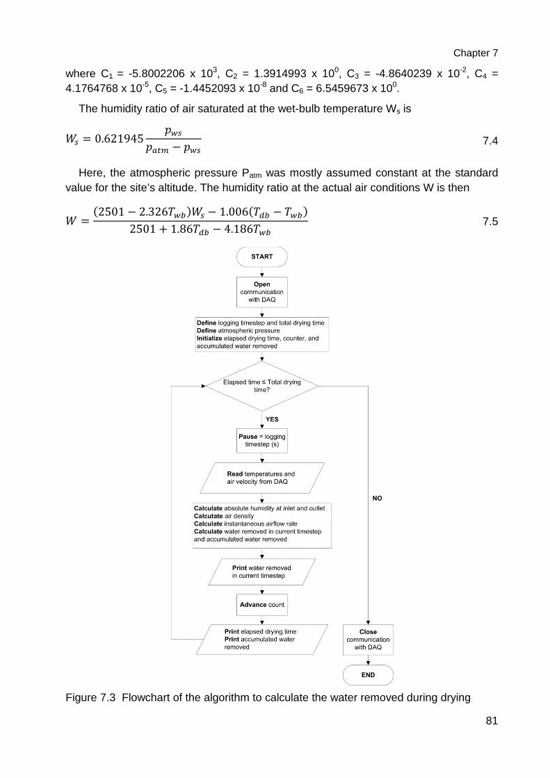
Chapter 7

81

where C1 = -5.8002206 x 103, C2 = 1.3914993 x 100, C3 = -4.8640239 x 10-2, C4 = 4.1764768 x 10-5, C5 = -1.4452093 x 10-8 and C6 = 6.5459673 x 100.

The humidity ratio of air saturated at the wet-bulb temperature Ws is

�T = 0.621945 'RT']^A − 'RT 7.4

Here, the atmospheric pressure Patm was mostly assumed constant at the standard value for the site’s altitude. The humidity ratio at the actual air conditions W is then

� = (2501 − 2.326)R�)�T − 1.006()�� − )R�)2501 + 1.86)�� − 4.186)R� 7.5

Figure 7.3 Flowchart of the algorithm to calculate the water removed during drying

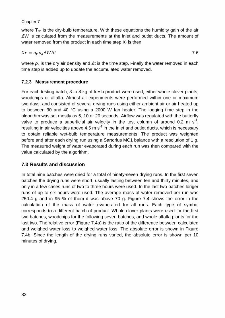
Chapter 7

82

where Tdb is the dry-bulb temperature. With these equations the humidity gain of the air ∆W is calculated from the measurements at the inlet and outlet ducts. The amount of water removed from the product in each time step Xr is then _` = YZP]∆�∆2 7.6

where ρa is the dry air density and ∆t is the time step. Finally the water removed in each time step is added up to update the accumulated water removed.

7.2.3 Measurement procedure

For each testing batch, 3 to 8 kg of fresh product were used, either whole clover plants, woodchips or alfalfa. Almost all experiments were performed within one or maximum two days, and consisted of several drying runs using either ambient air or air heated up to between 30 and 40 °C using a 2000 W fan heater. The logging time step in the algorithm was set mostly as 5, 10 or 20 seconds. Airflow was regulated with the butterfly valve to produce a superficial air velocity in the test column of around 0.2 m s-1, resulting in air velocities above 4.5 m s-1 in the inlet and outlet ducts, which is necessary to obtain reliable wet-bulb temperature measurements. The product was weighted before and after each drying run using a Sartorius MC1 balance with a resolution of 1 g. The measured weight of water evaporated during each run was then compared with the value calculated by the algorithm.

7.3 Results and discussion

In total nine batches were dried for a total of ninety-seven drying runs. In the first seven batches the drying runs were short, usually lasting between ten and thirty minutes, and only in a few cases runs of two to three hours were used. In the last two batches longer runs of up to six hours were used. The average mass of water removed per run was 250.4 g and in 95 % of them it was above 70 g. Figure 7.4 shows the error in the calculation of the mass of water evaporated for all runs. Each type of symbol corresponds to a different batch of product. Whole clover plants were used for the first two batches, woodchips for the following seven batches, and whole alfalfa plants for the last two. The relative error (Figure 7.4a) is the ratio of the difference between calculated and weighed water loss to weighed water loss. The absolute error is shown in Figure 7.4b. Since the length of the drying runs varied, the absolute error is shown per 10 minutes of drying.

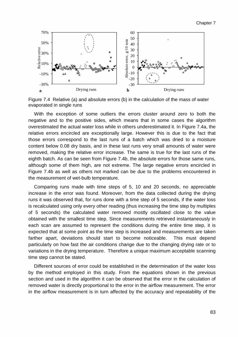
Chapter 7

83

Figure 7.4 Relative (a) and absolute errors (b) in the calculation of the mass of water evaporated in single runs

With the exception of some outliers the errors cluster around zero to both the negative and to the positive sides, which means that in some cases the algorithm overestimated the actual water loss while in others underestimated it. In Figure 7.4a, the relative errors encircled are exceptionally large. However this is due to the fact that those errors correspond to the last runs of a batch which was dried to a moisture content below 0.08 dry basis, and in these last runs very small amounts of water were removed, making the relative error increase. The same is true for the last runs of the eighth batch. As can be seen from Figure 7.4b, the absolute errors for those same runs, although some of them high, are not extreme. The large negative errors encircled in Figure 7.4b as well as others not marked can be due to the problems encountered in the measurement of wet-bulb temperature.

Comparing runs made with time steps of 5, 10 and 20 seconds, no appreciable increase in the error was found. Moreover, from the data collected during the drying runs it was observed that, for runs done with a time step of 5 seconds, if the water loss is recalculated using only every other reading (thus increasing the time step by multiples of 5 seconds) the calculated water removed mostly oscillated close to the value obtained with the smallest time step. Since measurements retrieved instantaneously in each scan are assumed to represent the conditions during the entire time step, it is expected that at some point as the time step is increased and measurements are taken farther apart, deviations should start to become noticeable. This must depend particularly on how fast the air conditions change due to the changing drying rate or to variations in the drying temperature. Therefore a unique maximum acceptable scanning time step cannot be stated.

Different sources of error could be established in the determination of the water loss by the method employed in this study. From the equations shown in the previous section and used in the algorithm it can be observed that the error in the calculation of removed water is directly proportional to the error in the airflow measurement. The error in the airflow measurement is in turn affected by the accuracy and repeatability of the

-30%

-10%

10%

30%

50%

70%

Re

lativ

e e

rro

r

Drying runsa-30-20-10

0102030405060

Ab

solu

te e

rro

r, g

/10

min

Drying runsb

Chapter 7

84

measurement device, the accuracy of the reference factor determined from the grid measurement, and the correct placement of the measurement probe during the trials.

As mentioned above, in most of this study it was assumed that atmospheric pressure remains constant at a standard value for the site. Although the calculation of air humidity ratio from psychrometric measurements is significantly affected by the atmospheric pressure (in the order of 10-4 kg kg-1 over the range of pressure variation in the site) since the useful quantity for the calculations in the algorithm is a difference of humidity ratios, the error by assuming constant pressure is reduced by about one order of magnitude. However, even these smaller errors can become significant for this application if the real and assumed atmospheric pressure differ enough. Part of the errors in Figure 7.4 might be attributed to this assumption. For the last two batches, although no real time measurements of atmospheric pressure could be carried out, its value was updated before every run when necessary, according to data available online from a meteorological station close to the site of the experiments.

The error that results from inaccuracies in the temperature measurements is more complex. It depends not only on the actual error in the measurement but also on the air conditions at the time, and whether the error occurs in a wet-bulb or a dry-bulb thermometer. The calculation of the humidity gain of the air is several times more sensitive to errors in the wet-bulb than in the dry-bulb temperature. Figure 7.5 shows the error in the calculated humidity ratio when an error of 0.1 °C occurs in only one of the temperature measurements. Here it can be observed that errors in the wet-bulb temperature are much more severe, and also that their effect increases with air temperature. The effect of errors in wet-bulb temperature also increases with the humidity ratio.

Figure 7.5 Errors in humidity ratio caused by a 0.1 °C error in dry or wet-bulb temperature

For an accurate measurement of wet-bulb temperature it is necessary that the wick wrapping the sensor tip is kept fully wet and that sensor and wick are in good contact with each other. Excessive wetting around the thermometer may make it indicate the water temperature, whilst if insufficiently wetted the thermometer may dry out, especially in hot air, so that the temperature readings will approach the dry-bulb value (Ustymczuk

0.00

0.05

0.10

0.15

0.20

10 30 50 70

erro

r in

hum

idity

rat

io,

g k

g-1

Dry bulb temperature, °C

error in Tdb error in Twb

Chapter 7

85

& Giner, 2011). It can be difficult by a simple inspection to verify and ensure that these conditions are met. Most of the error which took place in the experiments could be attributed to this problem. In the experimental set up the water level in the containers supplying water to the wick could not be kept constant automatically and after some time water had to be added to the containers. It became evident that relatively small variations in the water level already had an effect on the wet-bulb temperature measurement without the wick getting notoriously dry or so moist as to start dripping. This uncertainty required checking from time to time, and especially after long drying runs, if the measurements maintained their accuracy, which was not always the case. This was done running the apparatus while no product was placed in the drying column, so as to see if the difference between air humidity at the inlet and outlet of the apparatus calculated by the algorithm stayed nearly enough to zero, as it should be. Figure 7.6 shows two such empty runs. The time between scans was five seconds. A perfect measurement would result in an empty graph, but since measurement errors will always be present, ideally the difference should fluctuate around zero to both positive and negative sides in order to tend to cancel out and not accumulate. This occurred in Figure 7.6a and the average error in this case was -6.5 x 10-6 kg kg-1, which can be considered accurate enough. In Figure 7.6 the difference between inlet and outlet humidity was exclusively negative and the average error was -3.5 x 10-5 kg kg-1. It is possible that this cause of error is unimportant for other applications where air moisture measurements are required. For example, for air at a dry-bulb temperature of 25 °C and humidity ratio of 0.009 kg kg-1, an error in the wet-bulb temperature of 0.05 °C introduces an error of 5.98 x10-5 kg kg-1. In terms of relative humidity this corresponds to 0.3 percentage points, which may be considered accurate for meteorological data or any other application in which such measurements are used individually. However, in the present application this error, if kept constant during an entire drying batch, will accumulate and at the end of the process the difference between real average moisture and the calculation will be significant. Due to all this, special care must be taken in the wet-bulb temperature measurement. Sufficiently well constructed, wet-bulb thermometers are necessary in order to obtain results with the accuracy and the reliability demanded by this application.

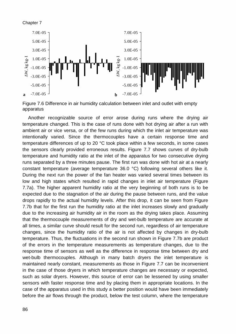
Chapter 7

86

Figure 7.6 Difference in air humidity calculation between inlet and outlet with empty apparatus

Another recognizable source of error arose during runs where the drying air temperature changed. This is the case of runs done with hot drying air after a run with ambient air or vice versa, or of the few runs during which the inlet air temperature was intentionally varied. Since the thermocouples have a certain response time and temperature differences of up to 20 °C took place within a few seconds, in some cases the sensors clearly provided erroneous results. Figure 7.7 shows curves of dry-bulb temperature and humidity ratio at the inlet of the apparatus for two consecutive drying runs separated by a three minutes pause. The first run was done with hot air at a nearly constant temperature (average temperature 36.0 °C) following several others like it. During the next run the power of the fan heater was varied several times between its low and high states which resulted in rapid changes in inlet air temperature (Figure 7.7a). The higher apparent humidity ratio at the very beginning of both runs is to be expected due to the stagnation of the air during the pause between runs, and the value drops rapidly to the actual humidity levels. After this drop, it can be seen from Figure 7.7b that for the first run the humidity ratio at the inlet increases slowly and gradually due to the increasing air humidity air in the room as the drying takes place. Assuming that the thermocouple measurements of dry and wet-bulb temperature are accurate at all times, a similar curve should result for the second run, regardless of air temperature changes, since the humidity ratio of the air is not affected by changes in dry-bulb temperature. Thus, the fluctuations in the second run shown in Figure 7.7b are product of the errors in the temperature measurements as temperature changes, due to the response time of sensors as well as the difference in response time between dry and wet-bulb thermocouples. Although in many batch dryers the inlet temperature is maintained nearly constant, measurements as those in Figure 7.7 can be inconvenient in the case of those dryers in which temperature changes are necessary or expected, such as solar dryers. However, this source of error can be lessened by using smaller sensors with faster response time and by placing them in appropriate locations. In the case of the apparatus used in this study a better position would have been immediately before the air flows through the product, below the test column, where the temperature

-7.0E-05

-5.0E-05

-3.0E-05

-1.0E-05

1.0E-05

3.0E-05

5.0E-05

7.0E-05

∆W

, kg

kg-1

a -7.0E-05

-5.0E-05

-3.0E-05

-1.0E-05

1.0E-05

3.0E-05

5.0E-05

7.0E-05

∆W

, kg

kg-1

b

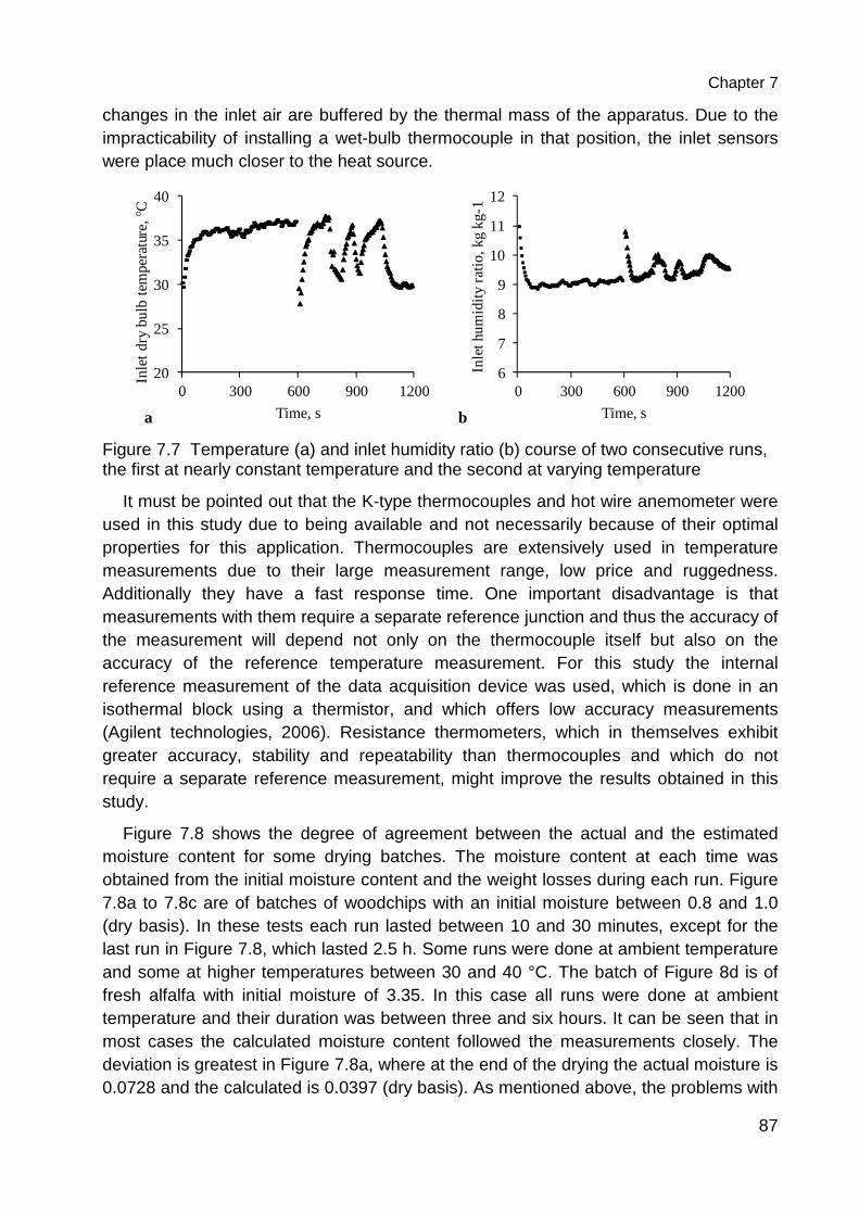
Chapter 7

87

changes in the inlet air are buffered by the thermal mass of the apparatus. Due to the impracticability of installing a wet-bulb thermocouple in that position, the inlet sensors were place much closer to the heat source.

Figure 7.7 Temperature (a) and inlet humidity ratio (b) course of two consecutive runs, the first at nearly constant temperature and the second at varying temperature

It must be pointed out that the K-type thermocouples and hot wire anemometer were used in this study due to being available and not necessarily because of their optimal properties for this application. Thermocouples are extensively used in temperature measurements due to their large measurement range, low price and ruggedness. Additionally they have a fast response time. One important disadvantage is that measurements with them require a separate reference junction and thus the accuracy of the measurement will depend not only on the thermocouple itself but also on the accuracy of the reference temperature measurement. For this study the internal reference measurement of the data acquisition device was used, which is done in an isothermal block using a thermistor, and which offers low accuracy measurements (Agilent technologies, 2006). Resistance thermometers, which in themselves exhibit greater accuracy, stability and repeatability than thermocouples and which do not require a separate reference measurement, might improve the results obtained in this study.

Figure 7.8 shows the degree of agreement between the actual and the estimated moisture content for some drying batches. The moisture content at each time was obtained from the initial moisture content and the weight losses during each run. Figure 7.8a to 7.8c are of batches of woodchips with an initial moisture between 0.8 and 1.0 (dry basis). In these tests each run lasted between 10 and 30 minutes, except for the last run in Figure 7.8, which lasted 2.5 h. Some runs were done at ambient temperature and some at higher temperatures between 30 and 40 °C. The batch of Figure 8d is of fresh alfalfa with initial moisture of 3.35. In this case all runs were done at ambient temperature and their duration was between three and six hours. It can be seen that in most cases the calculated moisture content followed the measurements closely. The deviation is greatest in Figure 7.8a, where at the end of the drying the actual moisture is 0.0728 and the calculated is 0.0397 (dry basis). As mentioned above, the problems with

20

25

30

35

40

0 300 600 900 1200

Inle

t d

ry b

ulb

tem

pera

ture

, °C

Time, sa

6

7

8

9

10

11

12

0 300 600 900 1200

Inle

t hu

mid

ity r

atio

, kg

kg-

1

Time, sb

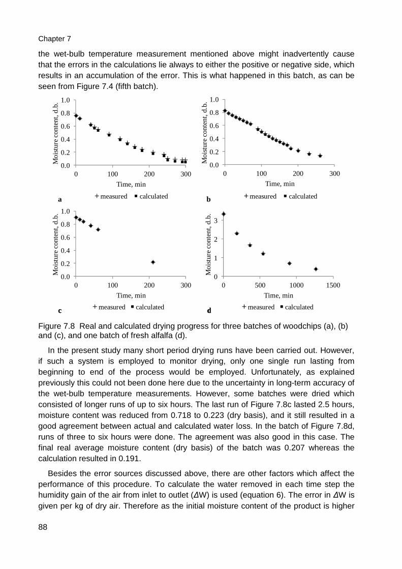
Chapter 7

88

the wet-bulb temperature measurement mentioned above might inadvertently cause that the errors in the calculations lie always to either the positive or negative side, which results in an accumulation of the error. This is what happened in this batch, as can be seen from Figure 7.4 (fifth batch).

Figure 7.8 Real and calculated drying progress for three batches of woodchips (a), (b) and (c), and one batch of fresh alfalfa (d).

In the present study many short period drying runs have been carried out. However, if such a system is employed to monitor drying, only one single run lasting from beginning to end of the process would be employed. Unfortunately, as explained previously this could not been done here due to the uncertainty in long-term accuracy of the wet-bulb temperature measurements. However, some batches were dried which consisted of longer runs of up to six hours. The last run of Figure 7.8c lasted 2.5 hours, moisture content was reduced from 0.718 to 0.223 (dry basis), and it still resulted in a good agreement between actual and calculated water loss. In the batch of Figure 7.8d, runs of three to six hours were done. The agreement was also good in this case. The final real average moisture content (dry basis) of the batch was 0.207 whereas the calculation resulted in 0.191.

Besides the error sources discussed above, there are other factors which affect the performance of this procedure. To calculate the water removed in each time step the humidity gain of the air from inlet to outlet (∆W) is used (equation 6). The error in ∆W is given per kg of dry air. Therefore as the initial moisture content of the product is higher

0.0

0.2

0.4

0.6

0.8

1.0

0 100 200 300

Mo

istu

re c

onte

nt,

d.b

.

Time, min

measured calculateda

0.0

0.2

0.4

0.6

0.8

1.0

0 100 200 300

Mo

istu

re c

onte

nt,

d.b

.

Time, min

measured calculatedb

0.0

0.2

0.4

0.6

0.8

1.0

0 100 200 300

Mo

istu

re c

onte

nt,

d.b

.

Time, min

measured calculatedcc

0

1

2

3

0 500 1000 1500

Mo

istu

re c

onte

nt,

d.b

.

Time, min

measured calculatedcd

Chapter 7

89

and its final moisture content lower, the error in the calculation may become more significant and unacceptably large, since more water must be removed and a larger mass of air is used. For example, the product in the batch of Figure 8d was freshly cut alfalfa with an initial moisture content of 3.35 (dry basis). If the same amount of alfalfa were dried in the field to 1.0, only about one third of the original moisture would need to be removed afterwards. Thus as the initial moisture content of the product increases the demands on accuracy are higher. As mentioned above, ideally the error in ∆W should closely resemble Figure 6a in order that the individual errors of each scan cancel each other out.

Similarly, at higher temperatures this procedure would be more accurate, since drying occurs at faster rates, each kg of air removes more water and therefore less air is needed in the process.

7.4 Conclusions

The results presented show that psychrometric and airflow measurements can be used to monitor the average moisture content of a product in batch dryers. However, several factors affect the accuracy of this methodology, all of which could not be adequately addressed in the present study. Attention must be given to sensor characteristics and location. Small deviations in temperature measurements, although negligible for other applications, might produce significant errors in this one. This is especially the case of wet-bulb temperature measurements, which are inherently difficult to perform with the accuracy and consistency required for this application. The unreliability of these measurements did not allow the execution of a drying batch in one single run of the algorithm, which is the final objective of this methodology. Due to the finite response time of temperature sensors, their location in the dryer or ducting system must be carefully chosen, particularly when drying conditions are expected to change rapidly. The use of four-wired resistance thermometers instead of thermocouples should be investigated since it could significantly improve the performance of this method. More tests in practical dryers are necessary.

90

8 General discussion

The present study was done in the framework of a research project entitled “Experimental investigation and demonstration of sorption energy storage facilities for the low-temperature solar drying”. The main characteristic of the sorption process directly relevant to the drying of agricultural products is the low temperature (some degrees above ambient), low humidity air resulting from its dehumidification by a concentrated, hygroscopic salt solution, which is afterwards concentrated again to be reused. Although a commercially ripe liquid desiccant system as the one being developed at the University of Kassel is not yet available, its application to crop drying is certainly possible and particularly interesting in the case of products which, to maintain a high quality (nutritional, medicinal, sensory or otherwise) need to be processed at relatively low temperature levels in which the drying rate is low. The disadvantage of using a low temperature can be at least partially offset by the humidity reduction of the drying air, which increases the difference in water vapor pressure between product and air.

8.1 Effect of air humidity on the drying behaviour of leaf celery

Although as expected the drying air temperature is the most important factor in the drying rate, air humidity also plays a role, particularly at low temperatures, which is important in drying systems with sorption storage. For other crops some studies have found a negligible effect of humidity or the effect was appreciable only at the upper end of the humidity range studied. When the effect was found only at high humidity, this might be due to the fact that at these high levels (above 60%), the equilibrium moisture content of the product was close to the aimed safe moisture content for the product (which is the one considered to determine the drying time) and the drying curve approaches this level asymptotically, thus overextending the drying. Other studies did not consider humidity as a factor at all. The results presented show that, keeping the temperature constant, the drying rate of the example product used (celery leaves) was influenced by humidity throughout the studied range which was from 10 to 60%. The highest temperature studied was 50 °C and here the effect is smaller due in part to the much shorter drying times needed to bring the product to a safe moisture level. Although these results cannot be generalized, it can be expected that air humidity has a similar effect on other plants at low drying temperatures.

8.2 Air distribution and drying uniformity in convective batch dryers

The results obtained both from CFD flow simulations and measurements show the importance of the air flow field in the drying uniformity in batch dryers. In the case of the box dryer, which is a slight variation of the more general fixed-bed dryer, the narrow inlet to the plenum chamber with its corresponding high velocity results in significant differences in air velocity through the product bulk. Although in this case the drying

General discussion

91

process was not simulated in dependence of this air distribution, it was expected that those zones with higher air velocities dried faster than zones with lower air velocities. If the total amount of product remains in the dryer until the slowest-drying box has reached the final moisture content, then a considerable waste of energy might occur by continuing the aeration of boxes in which no further drying takes place.

In view of the results obtained from CFD simulations in the original dryer, changes to the dryer geometry were tested using this tool and it was found that a widening of the air entrance to the plenum chamber in which air flows uniformly would result in an optimal air distribution through the product bulk. Given the small fan outlet a transition from 0.25 m to 1 m was required. A wide angle diffuser with a series of air guides and two perforated plates was chosen to fulfil this task.

The presence of boxes to hold the product allowed for an exact grid where measurements of air velocity and weight loss could be made. The high correlation found between the air flow through each box and its weight loss confirmed the theoretical predictions that those boxes with higher airflow rate would dry faster, and that improving the air distribution by making the air flow more uniform would impact positively the drying uniformity and therefore the dryer performance. Once the modifications were made to the physical dryer according to the simulation results, the air distribution and drying uniformity improved significantly. The standard deviation of the airflow in the boxes decreased by about 50% compared to the original dryer, and the drying curves of the individual boxes were much closer to each other. However, a completely uniform drying, in which all boxes dried at the same rate, did not occur. Although the initial moisture content of the product was assumed uniform for each test, actual variations in it could have caused these results. Also, temperature differences in the drying air might have played a role in this. The gas burners used to heat the air were located directly at the fan inlet, and the possibility that there existed temperature variations at this point which were carried with the flow, cannot be excluded. Unfortunately no such detailed temperature measurements were made in this study. Thus, besides focusing on air distribution, future studies should attempt to measure the homogeneity of the drying air temperature across the product bulk. Altogether, computational fluid dynamics has proven useful for the study of flow uniformity in convective dryers even if there were some differences between its results and measurements.

For round bale dryers, the flow simulations were complemented with the simulation of the drying process. In the case of the box dryer, since only the flow characteristics were considered, a full 3D simulation was possible and, due to its geometry, necessary. However, in the case of round bales, the implementation of the drying simulation made it necessary (due to lack of computational power available and time constraints) to simplify the problem to two dimensions in order to reduce the grid size and thus be able to carry out unsteady simulations. This, because the drying of round hay bales lasts, depending on the initial moisture content of the hay and the drying conditions, from several hours to more than a day, and the time step could not, in general, be chosen larger than two seconds, apparently due to numerical stability issues. Thus, the problem

General discussion

92

was reduced to a two-dimensional axisymmetric one. This simplification still results in a very good representation of the three dimensional problem provided that it can be assumed that the bale density is uniform in the circumferential direction.

The flow results showed important differences in the flow field in the different dryer designs. The simplest design, in which air enters the bale from one end, produced the most deficient air distribution in the bale. Here, the airflow decreases continuously along the bale height due to the higher resistance for the air to flow through longer paths of product bulk. The second design improved the air distribution, although not as significantly as was expected. The simulation of the bale drying was consistent with the flow field since it depends on it. It was seen that in the first two designs the drying front advanced upwards and outwards, but increasingly slowly as time passed. This is partly due to the decreased air flow reaching the upper bale region, but also due to the fact that, for a large period of time, the air reaching this region presents a very high humidity, close to saturation, so that virtually no drying takes place there until later in the process. In both these designs, this results, after some time of drying, in large moisture gradients in the bale, with some regions at equilibrium with the inlet air conditions, and others at the initial moisture content, so that even if the average moisture content of the bale is below the safe level for storage, large portions of it would still be at levels high enough for mold development, self-heating and overall quality loss. Thus, in the case of the first and second designs turning the bales after some time would serve to speed up the process, reduce energy waste and increase the efficiency. On the other hand, the turning of the bales may or may not be problematic or at least it could require considerable time depending on the available machinery and the size of the drying facility.

The third drying design proved to be the optimal solution provided that the radial void can be consistently produced in round bales and that the bale presents a uniform enough density distribution along its height and also around its circumference. Otherwise, as evident from the results, pronounced density variations reduce significantly the superiority of this design. The fourth design, in which the air enters the bale through both ends is also superior to the first two, so that no large moisture gradients develop.

The experimental tests showed a drying behaviour similar to the simulations, although in some cases some differences occurred. This was particularly evident in the case of the first design, in which sometimes the flow distribution and the drying progress did not follow the simulation results as expected. A problem in testing actual round bales is that, due to the nature of the product and the process by which it is obtained, all bales differ, to a higher or lesser degree, from one another in terms of size, initial weight, initial moisture content and density distribution. Even within one bale, the initial moisture content will vary randomly, sometimes significantly, since the crop is first dried partially in the field whereas for simulations, in the absence of better initial conditions, uniform initial moisture content was assumed. The variation in the dry matter density in the bale, which was mentioned above, also contributed to the difficulty in comparing

General discussion

93

experimental and simulation results. Although it was attempted during the tests to minimize density variations, the result was often unsatisfactory and seemed to depend strongly not only on the baler, but also on the hay rake and the shape of the windrow. The factors mentioned above not only may have contributed to differences between simulation and measurements but it also created difficulty in comparing between experimental tests and designs. Unfortunately, the number of experimental tests done was somewhat limited due to logistic issues. Nonetheless, as was the case with the box dryer, CFD has been useful tool to study the flow behaviour in compressed bulks like round bales which present a partially random density distribution. Also, as it was seen, the simulation of the drying process can be implemented in the software with relative ease and thus a more complete description of the process is obtained.

The temperature measurements made at several positions in the bale interior and the use of an infrared camera to measure the bale surface temperature are suitable techniques to follow the drying process and its uniformity since the temperature of air and product in a bulk being dried is related to the moisture content.

8.3 Real-time moisture content monitoring

The use of psychrometric and airflow measurements is a feasible method for the monitoring of the drying process in batch dryers, provided some conditions are met by the system. Although in this work only preliminary tests were performed, the results are promising since the accuracy achieved was satisfactory. However, various possible error sources were identified. Perhaps the most critical is the measurement of wet-bulb temperature, since its correct measurement is in itself more complicated, and because the calculation of air humidity is several times more sensitive to errors in it than to errors in dry-bulb temperature.

It was also seen that variations in the inlet air temperature resulted in inaccuracies in the measurement of air humidity, which was due to the finite response time of the thermocouples but also the difference in the response time between them. Therefore, a simple measure to minimize this error would be to install sensors with a response time as short as possible, for example using sensors with smaller diameters, but considering also a minimum of ruggedness.

8.4 Further research

The study done in this research on the effect of relative humidity in the drying behaviour at low air temperatures (Chapter 4) was of limited scope. It involved only a single example product, and on a thin-layer. Most herb and hay drying takes place on deeper beds, and ultimately it is in such beds that a comparison of the effect of different air conditioning methods should be done in the future. Also, the low temperature, low humidity conditions studied in this work were those which could be obtained from the ambient conditions without the actual dehumidifying which would take place in the liquid desiccant system. Therefore, air conditions produced by the sorption process will

General discussion

94

include others not considered here and a study under a broader range of conditions and for different products should be aimed at. This can be done experimentally and also by computer simulations using self-written drying programs or CFD software, provided the necessary information is available.

Flow and drying simulations in fixed-bed dryers, accompanied by experimental measurements, should also be done on dryer types and geometries other than that of Chapter 5. For example, some dryers are fitted with means to reverse the direction of airflow in order to reduce moisture gradients in the product bulk. Such dryers are amenable to simulation using CFD and valuable information can be obtained with respect to their performance relative to more conventional dryers and about the optimization of the airflow reversal method.

As was shown in Chapter 6, success in the drying of hay in round bales depends as much on the dryer design as on their dry matter density distribution, which ideally should be uniform along the bale axis and around its circumference. Thus, an important area of further study is the consistent production of round bales adequate for drying. This requires consideration of several field operations, including at least raking and baling, and the machinery and methods employed.

In order to optimize the method for moisture content monitoring studied in Chapter 7, further tests should be carried out in practical batch dryers. Different sensor types and sensor locations should be tried.

95

9 Summary

Drying is one of the most used operations to extend the shelf life of agricultural products. Among the many types of technologies, convective drying using air as the energy and mass carrier remains the most important for agricultural products. In batch dryers a fixed amount of product is dried from its initial to its final moisture content before the system is unloaded and loaded again with moist product. Despite their shortcomings and high specific energy consumption, they are still widely used for drying of grain, herbs and spices. Also, when hay is dried artificially, convective batch dryers are ubiquitous.

The present work took place in the framework of a research project investigating a liquid desiccant solar energy storage system for the drying of agricultural products. From the agricultural engineering part, the focus was on the drying of crops at the low air temperature and humidity levels delivered by the sorption system and in the study and improvement of air distribution and drying uniformity in dryers for medicinal plants and hay.

Thin-layer drying experiments were conducted at varying air temperature (20-50 °C) and relative humidity (10-60%) using leaf celery as example, in order to investigate the effect of this process parameters on the drying rate and the final color of the product. Additionally, and for a correct evaluation of the drying characteristics, sorption isotherms of this crop were also determined using the gravimetric method in which a product sample is kept in environments of different relative humidity (11-84%) and temperature (25-50 °C) using saturated salt solutions. Results were clear in the importance of air temperature in the drying rate of leaf celery in the range of temperature studied, and agree well with studies performed with other crops. In going from 20 to 50 °C the drying time reduces by one order of magnitude. Most importantly, the data showed that relative humidity also plays a role on the drying rate, for which the literature does not provide with a definite position. At 40 °C the color of the dried product remained green when relative humidity was up to 45%; however, when humidity was 60% the color was affected and brown regions appeared in the leaves. At 50 °C the leaves turned brown throughout the humidity range.

The study of air distribution in a fixed-bed, box dryer was done through experiments and through flow simulations using computational fluid dynamics (CFD). The software ANSYS Fluent 12 was used to perform 3D and 2D simulations of air flow in the box dryer, which was constructed in the workshop in parallel. This dryer had a simple duct joining the centrifugal fan to the plenum chamber, as it occurs most commonly in practical dryers. The airflow through each of the thirty-six boxes carrying product was estimated by measuring the air velocity at the smaller end of a tapered channel. The drying in the individual boxes was monitored at specified intervals. Three experiments were carried out with this dryer configuration with an air temperature of 50-65 °C. Both simulation and experimental results showed that this configuration provides a deficient

Summary

96

air distribution. The drying rate in the boxes varied greatly and it was strongly correlated to the airflow. Further flow simulations indicated that a modification of the dryer consisting of a wide entrance to the plenum chamber with a uniform air velocity would produce a nearly perfect air distribution through all the boxes. It was found that a short, wide-angle diffuser fitted with eight air guides and two perforated plates to serve as transition between fan and plenum chamber would fulfill this. Three experiments conducted with the so modified dryer confirmed the expected improvement in dryer performance. The variation (as standard deviation) in the airflow through the boxes decreased by 50%, and drying uniformity also improved substantially. Thus, the use of an adequate diffuser as a transition element is an effective design change to improve the air distribution and drying uniformity in batch dryers like the studied in this work.

For the study of round bale dryers the same methodology was used as for the box dryer. However in this case a drying model was implemented in the CFD software to simulate the drying process in dependence of the air flow in the bale. This was done through user-defined functions (UDF) and the definition of a user-defined scalar (UDS) as the air humidity transported in the flow, as well as by introducing new variables. A well formed bale and a suboptimal one were modelled using constant or variable dry matter density along the bale axis, and the porosity and air resistance of the bale was varied accordingly. The simulations were performed in 2D axisymmetric flow. Four bale dryer designs were considered. In the first design air flows into the bale through one end while the other end is closed. The second design is similar to the first but the lower 0.5 m of the bale lateral surface is covered. The air distribution in both cases was deficient, with very little air reaching the upper bale region. The drying simulations for both designs showed that after 7 hours of drying at 38 °C and with an airflow rate of 0.5 m3 s-1 the bales still had 31.2 and 23.4% of their volume at a moisture content above 15% in wet basis (w.b.) respectively, with some regions even at the initial moisture of 30%. Therefore a much longer drying time was needed to bring down the moisture content of the entire bale to a safe level. This makes the turning of the bales at some point during drying necessary to reduce drying time and avoid unnecessary energy waste. For the third design, in which air flows radially from the bale axis to the surface, only 1.7% of the bale volume had a moisture level above 15% (w.b.). In this design the air distribution and drying uniformity when the bale is well formed was optimal, but the results also showed that its performance deteriorates significantly when the bale presents a non-uniform dry matter density along its axis, as it occurs often in practice. The fourth design, in which air enters the bale through both ends, also resulted in an improved drying uniformity, with 8.8% of the bale volume over 15% (w.b.) after 7 hours of drying. Drying tests were conducted on the first three designs mentioned above and measurements showed good agreement with simulation results, although in some cases differences appeared. Thus, computational fluid dynamics software has proven to be a useful tool in evaluating convective drying systems and in gaining insight on the process, especially if the drying simulation is implemented. The internal bale temperature at various positions and infrared images are useful in judging the extent and uniformity of bale drying.

Summary

97

The continuous moisture content monitoring in batch dryers by use of psychrometric and airflow measurements was tested experimentally to assess its feasibility. A laboratory test rig for air resistance experiments was modified to serve as a batch dryer and the necessary sensors were installed. Two pairs of K-type thermocouples were used to form two psychrometers to measure inlet and outlet humidity of the drying air. Airflow was estimated from a single point measurement of air velocity at the inlet duct and by applying a correction factor obtained from a grid measurement in the same cross section. An algorithm written in MATLAB allowed the communication with the DAQ, the retrieval of the sensors signals at short, specified time intervals, and performed the calculations to estimate the water removed from the test product. The actual and the estimated water removed were in good agreement in most cases, showing that this method can be successfully applied to monitor the drying progress. However, some conditions must be met by the dryer and the sensors.

98

10 Zusammenfassung

Die Trocknung ist eines der am Häufigsten benutzten Verfahren, um die Haltbarkeit von landwirtschaftlichen Gütern zu verlängern. Von den vielen gebräuchlichen Trocknungsarten ist die Konvektionstrocknung die wichtigste. Im Satztrockner wird eine bestimmte Produktmenge von ihrer Anfangs- bis zu ihrer Endfeuchte getrocknet, bevor das System entladen wird und ein neuer Zyklus beginnt. Trotz ihrer Nachteile und ihres hohen spezifischen Energieverbrauchs ist sie für Getreide-, Kräuter- und Heutrocknung noch weit verbreitet.

Diese Arbeit fand in Rahmen eines Forschungsprojekts statt, das eine sorptionsgestützte solare Trocknung von landwirtschaftlichen Gütern untersuchte. Im agrartechnischen Teil lag der Schwerpunkt auf der Trocknung bei niedriger Temperatur und geringer Feuchte, die der Sorptionsprozess liefert, und auf der Verbesserung der Luftverteilung sowie der Gleichmäßigkeit der Trocknung im Kräuter- und Heutrockner.

Dünn-Schicht Trocknungsversuche wurden bei verschiedenen Temperaturen (20-50 °C) und relativen Feuchten (10-60 %) durchgeführt, mit Schnitt-Sellerie als Beispielprodukt. Damit war es möglich, den Einfluss dieser Prozessvariablen auf die Trocknungsgeschwindigkeit und Endfarbe des Produktes zu untersuchen. Um die korrekten Trocknungseigenschaften zu ermitteln, wurden die Sorptionsisothermen dieser Pflanze auch mit der gravimetrischen Methode bestimmt. Hierbei wurden Produktproben in Umgebungen verschiedener relativer Feuchten (11-84 %) und Temperaturen (25-50 °C) gehalten, wobei gesättigte Salzlösungen benutzt wurden. Die Ergebnisse zeigten eindeutig den Einfluss der Lufttemperatur auf die Trocknung von Schnitt-Sellerie in dem untersuchten Temperaturbereich und stimmen mit Untersuchungen an anderen Produkten überein. Die Trocknung bei 50 °C ist um eine Größenordnung schneller als bei 20 °C. Darüber hinaus zeigten die Ergebnisse, dass die relative Luftfeuchte auch eine Rolle in der Trocknungsgeschwindigkeit spielt, wozu es in der Literatur keine eindeutigen Aussagen gibt. Bei 40 °C und 45 % relativer Feuchte blieb die grüne Farbe beim Endprodukt erhalten. Dagegen zeigte sich bei einer Feuchte von 60 % eine Beeinträchtigung der Farbe und es bildeten sich braune Flecken. Bei 50 °C wurden die Blätter durchgehend braun, unabhängig von der Luftfeuchte.

Die Untersuchung der Luftverteilung in einem Festbett-Kistentrockner wurde experimentell sowie mit Hilfe von numerischer Strömungsberechnung durchgeführt. Das Programm ANSYS Fluent 12 wurde für zwei- und drei-dimensionale Luftströmungssimulationen benutzt, und parallel wurde in der Werkstatt ein Kistentrockner gebaut. Dieser Trockner hatte, wie in Trocknern praxisüblich, einen einfachen Luftkanal, der den Radiallüfter mit der Luftkammer verbindet. Die Luftverteilung in den 36 produktbeladenen Kisten wurde mit Hilfe eines sich verjüngenden Kanals gemessen. Der Trocknungsfortschritt der einzelne Kisten wurde in regelmäßigen Zeitabständen überwacht. Mit dieser Trockneranordnung wurden drei

Zusammenfassung

99

Versuche bei einer Lufttemperatur von 50-65 °C durchgeführt. Experimentelle sowie numerische Ergebnissen zeigten, dass diese Trocknerkonfiguration eine mangelhafte Luftverteilung liefert. Die Trocknungsgeschwindigkeit der Kisten war sehr unterschiedlich und korrelierte stark mit dem Luftvolumenstrom. Weitere Strömungssimulationen zeigten, dass eine Veränderung des Trockners durch einen breiten Eingang zur Luftkammer und eine gleichbleibende Luftgeschwindigkeit eine nahezu gleichmäßige Luftverteilung zu allen Kisten ermöglicht. Laut Simulationen würde ein kurzer, weitwinkliger, mit acht Leitblechen und zwei Lochblechen ausgestatteter Diffusor als Übergang zwischen Lüfter und Luftkammer diese Funktion erfüllen. In drei Trocknungsversuchen mit dieser veränderten Trockneranordnung wurde die erwartete Verbesserung bestätigt. Die Streuung (als Standardabweichung) des Luftvolumenstroms durch die Kisten verringerte sich um 50 % und die Gleichmäßigkeit der Trocknung verbesserte sich substantiell. Daraus folgt, dass der Einsatz eines angepassten Diffusors als Übergangselement eine effektive Veränderung des Designs darstellt, um die Luftverteilung und Gleichmäßigkeit der Trocknung in Kistentrocknern wie den in dieser Arbeit untersuchten zu verbessern.

Für die Untersuchung von Rundballentrocknern wurde die gleiche Methodik angewendet wie für den Kistentrockner. Allerdings wurde in diesem Fall ein Trocknungsmodell in die CFD Software eingefügt, um den Trocknungsprozess in Abhängigkeit von der Luftzirkulation im Ballen zu simulieren. Dies wurde durch nutzerdefinierte Funktionen (UDF) und die Festlegung eines nutzerdefinierten Skalars für die im Luftstrom transportierte Feuchte wie auch durch die Einführung neuer Variablen erreicht. Ein gut geformter (gepresster) und ein suboptimaler Ballen wurden unter Nutzung konstanter oder variabler Trockenmassendichte entlang der Ballenachse modelliert, dazu wurden die Durchlässigkeit und der Luftwiderstand des Ballens entsprechend variiert. Die Simulationen wurden in 2D achsensymmetrischer Strömung durchgeführt. Vier Ballentrocknerdesigns wurden betrachtet. Bei dem ersten strömt die Luft auf der einen Seite ein, während die andere abgedichtet ist. Das zweite ist ähnlich dem ersten, aber die unteren 0,5 m der Ballenseitenfläche werden bedeckt. Die Luftverteilung war in beiden Varianten unzulänglich, nur sehr wenig Luft erreichte die obere Region der Ballen. Die Trocknungssimulation zeigte für beide Designs, dass die Ballen nach 7 Stunden Trocknung mit 38 °C und mit einer Luftstromrate von 0,5 m³ s-1 in 31,2% bzw. 23,4% ihres Volumens noch einen Feuchtegehalt von über 15% hatten, in einigen Bereichen sogar den Ausgangsfeuchtegehalt von 30%. Daher wurde eine viel längere Trocknungszeit benötigt, um den Feuchtegehalt des gesamten Ballens bis zu einem sicheren Niveau herunterzubringen. Daraus erwächst die Notwendigkeit, die Ballen während des Trocknens umzudrehen, um die Trocknungszeit zu verkürzen und unnötige Energieverschwendung zu vermeiden. Im dritten Trocknerdesign, in dem die Luft radial von der Ballenachse bis zum Ballenmantel fließt, hätte nach sieben Stunden Trocknungszeit bei den oben genannten Bedingungen nur 1,7 % des Ballenvolumen einen Feuchtegehalt von über 15 %. In diesem Fall waren die Luftverteilung und die Gleichmäßigkeit der Trocknung optimal, wenn der Ballen auch optimal gepresst war. Allerdings zeigten die Ergebnisse auch, dass bei ungleichmäßiger Dichteverteilung der

Zusammenfassung

100

Ballen in axialer Richtung, wie das in der Praxis meistens der Fall ist, dieses Design wesentlich schlechtere Ergebnisse bringt. Das vierte Design, in dem die Luft durch beide Ballenseiten fließt, zeigte auch eine verbesserte Trocknungsgleichmäßigkeit, mit nur 8,8 % des Ballenvolumens über 15 % Feuchte nach sieben Stunden Trocknung. Trocknungsversuche wurden für die ersten drei Trocknerdesigns durchgeführt und die Messungen zeigten eine gute Übereinstimmung mit den Simulationen, obwohl in manchen Fällen klare Unterschiede auftraten. Daraus folgt, dass die computergestützte Strömungsdynamik-Software ein nützliches Werkzeug ist, um Konvektionstrocknungssysteme zu bewerten und Einblicke in den Prozess zu gewinnen, besonders wenn die Trocknungssimulation einbezogen wird. Die Balleninnentemperatur an verschiedenen Stellen und Infrarotbilder sind nützlich, um das Maß und die Gleichförmigkeit der Ballentrocknung beurteilen zu können.

Eine kontinuierliche Feuchtegehaltskontrolle in Kistentrocknern durch psychometrische und Luftstrommessungen wurde experimentell getestet, um deren Umsetzbarkeit bewerten zu können. Eine Labortesteinrichtung für Luftwiderstandsversuche wurde modifiziert, um einen Satztrockner darzustellen und die nötigen Sensoren wurden angebracht. Zwei Paare K-Typ Thermoelemente wurden als Psychrometer eingesetzt, um die Eingangs- und Ausgangsfeuchte der Trocknungsluft zu messen. Der Luftvolumenstrom wurde aus einer Einpunktmessung der Luftgeschwindigkeit am Eingangskanal und mit Anwendung eines von einer Netzmessung erhaltenen Korrekturfaktors kalkuliert. Ein in MATLAB geschriebener Algorithmus erlaubte die Kommunikation mit dem Datenerfassungsgerät, die Entnahme der Sensorensignale in kurzen, festgelegten Zeitintervallen, und führte die Berechnungen für die Abschätzung der dem Produkt entzogenen Wassermenge durch. Die tatsächliche und abgeschätzte entfernte Wassermenge waren meistens in guter Übereinstimmung, was zeigte, dass diese Methode erfolgreich einzusetzen ist, um den Trocknungsverlauf zu überwachen. Allerdings müssen von Trockner und Sensoren bestimmte Bedingungen erfüllt werden.

101

11 References

Adler, A. (2002). Qualität von Futterkonserven und mikrobielle Kontamination. In 8. Alpenländisches Expertenforum (pp. 17–26). Irdning: Bundesanstalt für alpenländische Landwirtschaft Gumpenstein.

Agilent technologies. (2006). Agilent 34970A Data Acquisition / Switch Unit User’s Guide. Agilent Technologies, Inc.

Ajibola, O. O. (1989). Thin-layer drying of melon seed. Journal of Food Engineering, 9(4), 305–320. doi:10.1016/0260-8774(89)90037-X

Amanlou, Y., & Zomorodian, a. (2010). Applying CFD for designing a new fruit cabinet dryer. Journal of Food Engineering, 101(1), 8–15. doi:10.1016/j.jfoodeng.2010.06.001

ANSYS. (2009). ANSYS Fluent 12.0 User´s Guide. ANSYS.

Arabhosseini, A., Huisman, W., van Boxtel, A., & Müller, J. (2006). Sorption isotherms of tarragon (Artemisia dracunculus L.). Zeitschrift Für Arznei- Und Gewürzpflanzen, 11(1), 48–51.

Arabhosseini, A., Huisman, W., van Boxtel, A., & Müller, J. (2009). Modeling of thin layer drying of tarragon (Artemisia dracunculus L.). Industrial Crops and Products, 29(1), 53–59. doi:10.1016/j.indcrop.2008.04.005

Argyropoulos, D., & Müller, J. (2011). Effect of convective drying on quality of lemon balm (Melissa officinalis L.). In Procedia Food Science (Vol. 1, pp. 1932–1939). doi:10.1016/j.profoo.2011.09.284

Arinze, E. A., Sokhansanj, S., Schoenau, G. J., & Trauttmansdorf, F. G. (1996). Experimental evaluation, simulation and optimization of a commercial heated-air batch hay drier: Part 1, drier functional performance, product quality, and economic analysis of drying. Journal of Agricultural Engineering Research, 63(4), 301–314.

ASABE. (2008). ASAE D245.6 Moisture relationships of plant-based agricultural products. ASABE.

ASHRAE. (2009). Psychrometrics. In ASHRAE Handbook - Fundamentals (p. 16). American Society of Heating, Refrigerating and Air-Conditioning Engineers.

Bahloul, N., Boudhrioua, N., & Kechaou, N. (2008). Moisture desorption–adsorption isotherms and isosteric heats of sorption of Tunisian olive leaves (Olea europaea L.). Industrial Crops and Products, 28(2), 162–176. doi:10.1016/j.indcrop.2008.02.003

References

102

Belghit, A., Kouhila, M., & Boutaleb, B. C. (2000). Experimental study of drying kinetics by forced convection of aromatic plants. Energy Conversion and Management, 41(12), 1303–1321. doi:10.1016/S0196-8904(99)00162-4

Bohl, W., & Elmendorf, W. (2008). Technische Strömungslehre (14th ed., p. 504). Würzburg: Vogel Verlag Und Druck.

Brandemuehl, S. L., Straub, R. J., Koegel, R. G., Shinners, K. J., & Fronczak, F. J. (1988). Radial drying of high moisture, large round hay bales. In International Summer Meeting of the American Society of Agricultural Engineers (pp. 1–18). Rapid City: ASAE.

Briens, L., & Bojarra, M. (2010). Monitoring fluidized bed drying of pharmaceutical granules. AAPS PharmSciTech, 11(4), 1612–8. doi:10.1208/s12249-010-9538-1

Brooker, D. B., Bakker-Arkema, F. W., & Hall, C. W. (1992). Drying and storage of grains and oilseeds (1st ed., p. 450). New York: Springer.

Buckmaster, D. R., Rotz, C. A., & Mertens, D. R. (1989). A model of alfalfa hay storage. Transactions of the ASAE, 32(1), 30–36.

Chaplin, G., Pugsley, T., & Winters, C. (2005). Monitoring the fluidized bed granulation process based on S-statistic analysis of a pressure time series. AAPS PharmSciTech, 6(2), E198–201. doi:10.1208/pt060229

Chiumenti, R., Da Borso, F., & Donantoni, L. (1997). Essiccazione artificiale di rotoballe di medica (Medicago sativa L.): verifiche sperimentali sulla funzionalità degli impianti. Rivista Di Agronomia, 31(1), 291–294.

Corrêa, P. C., Martins, J. H., & Christ, D. (1999). Thin layer Drying Rate and Loss of Viability Modelling for Rapeseed (Canola). Journal of Agricultural Engineering Research, 74(1), 33–39. doi:10.1006/jaer.1999.0430

Correa-Hernando, E., Arranz, F. J., Diezma, B., Juliá, E., Robla, J. I., Ruiz-Garcia, L., … Barreiro, P. (2011). Development of model based sensors for the supervision of a solar dryer. Computers and Electronics in Agriculture, 78(2), 167–175. doi:10.1016/j.compag.2011.07.004

Da Silva, F., Park, K. J., Magalhães, P. M., & Pozitano, M. (2004). Desorption isotherms of Calendula oficinalis L. In 14th International Drying Symposium (Vol. C, pp. 1569–1576). Sao Paulo.

Dandamrongrak, R., Young, G., & Mason, R. (2002). Evaluation of various pre-treatments for the dehydration of banana and selection of suitable drying models. Journal of Food Engineering, 55(2), 139–146. doi:10.1016/S0260-8774(02)00028-6

DLG. (2007). Rundballenpresse Fendt 2900 VS – Durchsatz und Pressdichte (pp. 1–8). Retrieved from http://www.dlg-test.de/pbdocs/5717F.pdf.

References

103

Doymaz, İ. (2011). Drying of thyme (Thymus vulgaris L.) and selection of a suitable thin-layer drying model. Journal of Food Processing and Preservation, 35(4), 458–465. doi:10.1111/j.1745-4549.2010.00488.x

Fonnesbeck, P. V., de Hernandez, M. M. G., Kaykay, J. M., & Saiady, M. Y. (1986). Estimating yield and nutrient losses due to rainfall on field-drying alfalfa hay. Animal Feed Science and Technology, 16(1-2), 7–15. doi:10.1016/0377-8401(86)90045-3

Gindl, G. (2002). Zeitgemäße Heubereitung und Heuqualität in der Praxis. In 8. Alpenländisches Expertenforum (pp. 67–72). Irdning: Bundesanstalt für alpenländische Landwirtschaft Gumpenstein.

Godsalve, E. W., Davis, E. A., Gordon, J., & Davis, H. T. (1977). Water loss rates and temperature profiles of dry cooked bovine muscle. Journal of Food Science, 42(4), 1038–1045. doi:10.1111/j.1365-2621.1977.tb12662.x

Heindl, A., & Müller, J. (1997). Trocknung von Arznei- und Gewürzpflanzen. Zeitschrift Für Arznei- Und Gewürzpflanzen, 2(2), 90–97.

Holpp, M. (2004). Trocknung von Rundballen: Machbarkeit und Wirtschaftlichkeit. FAT Berichte (Nr. 616) (pp. 1–12).

Hoppe, B. (2005). Studie zum Stand des Anbaus von Arznei- und Gewürzpflanzen in Deutschland (2003) und Abschätzung der Entwicklungstrends in den Folgejahren (pp. 1–26). Bernburg.

Hosseini, A. A. M. (2005). Quality, energy requirement and costs of drying tarragon (Artemisia dracunculus L.). Ph.D. Thesis. Wageningen University.

Iglesias, H. A., & Chirife, J. (1982). Handbook of food isotherms: water sorption parameters for food and food components (p. 350). New York: Academic Press.

Jamali, A., Kouhila, M., Ait Mohamed, L., Idlimam, A., & Lamharrar, A. (2006). Moisture adsorption–desorption isotherms of Citrus reticulata leaves at three temperatures. Journal of Food Engineering, 77(1), 71–78. doi:10.1016/j.jfoodeng.2005.06.045

Janjai, S., Intawee, P., Chaichoet, C., Mahayothee, B., Haewsungcharern, M., & Müller, J. (2006). Improvement of the air flow and temperature distribution in a conventional longan dryer. In International Symposium Towards Sustainable Livelihoods and Ecosystems un Mountaneous Regions. Chiang Mai.

Jayas, D. S., & Muir, W. E. (2002). Aeration systems design. In S. Navarro & R. Noyes (Eds.), The mechanics and physics of modern grain aeration management (1st ed., pp. 195–249). Boca Raton: CRC Press Inc.

Kashaninejad, M., Mortazavi, a., Safekordi, a., & Tabil, L. G. (2007). Thin-layer drying characteristics and modeling of pistachio nuts. Journal of Food Engineering, 78(1), 98–108. doi:10.1016/j.jfoodeng.2005.09.007

References

104

Khatchatourian, O. a. (2012). Experimental study and mathematical model for soya bean drying in thin layer. Biosystems Engineering, 113(1), 54–64. doi:10.1016/j.biosystemseng.2012.06.006

Kouhila, M., Belghit, A., Daguenet, M., & Boutaleb, B. . (2001). Experimental determination of the sorption isotherms of mint (Mentha viridis), sage (Salvia officinalis) and verbena (Lippia citriodora). Journal of Food Engineering, 47(4), 281–287. doi:10.1016/S0260-8774(00)00130-8

Kröll, K. (1997). Trocknungstechnik Zweiter band - Trockner und Trocknungsverfahren (2nd ed., p. 654). Berlin: Springer.

Lamond, W. J., & Graham, R. (1993). The relationship between the qeuilibrium moisture content of grass mixtures and the temperature and humidity of the air. Journal of Agricultural Engineering Research, 56(4), 327–335. doi:10.1006/jaer.1993.1083

Lawrence, J., & Maier, D. E. (2012). Prediction of temperature distributions in peaked, leveled and inverted cone grain mass configurations during aeration of corn. Applied Engineering in Agriculture, 28(5), 685–692.

Lewis, W. K. (1921). The rate of drying of solid materials. Journal of Industrial and Engineering Chemistry, 13(5), 427–432.

Liendo-Cárdenas, M., Zapata-Norena, C. P., & Brandelli, A. (2000). Sorption isotherm equations of potato flakes and sweet potato flakes. Brazilian Journal of Food Technology, 3, 53–57.

Madamba, P. S., Driscoll, R. H., & Buckle, K. A. (1996). The thin-layer drying characteristics of garlic slices. Journal of Food Engineering, 29(1), 75–97. doi:10.1016/0260-8774(95)00062-3

Margaris, D. P., & Ghiaus, A.-G. (2006). Dried product quality improvement by air flow manipulation in tray dryers. Journal of Food Engineering, 75(4), 542–550. doi:10.1016/j.jfoodeng.2005.04.037

Mathioulakis, E., Karathanos, V. T., & Belessiotis, V. G. (1998). Simulation of air movement in a dryer by computational fluid dynamics: Application for the drying of fruits. Journal of Food Engineering, 36(2), 183–200. doi:10.1016/S0260-8774(98)00026-0

Mehta, S., & Singh, A. (2006). Adsorption isotherms for red chilli (Capsicum annum L.). European Food Research and Technology, 223(6), 849–852. doi:10.1007/s00217-006-0279-z

Mellmann, J., & Fürll, C. (2008). Trocknungsanlagen für Arznei- und Gewürzpflanzen - spezifischer Energieverbrauch und Optimierungspotential. Zeitschrift Für Arznei- Und Gewürzpflanzen, 13(3), 127–133.

References

105

Menkov, N. D. (2000). Moisture sorption isotherms of chickpea seeds at several temperatures. Journal of Food Engineering, 45(4), 189–194. doi:10.1016/S0260-8774(00)00052-2

Menzies, D. J., & O’Callaghan, J. R. (1971). The effect of temperature on the drying rate of grass. Journal of Agricultural Engineering Research, 16(3), 213–222. doi:10.1016/S0021-8634(71)80015-X

Mielke, H., & Schöber-Butin, B. (2007). Heil- und Gewürzpflanzen - Anbau und Verwendung (p. 288). Berlin: Biologische Bundesanstalt für Land- und Forstwirtschaft.

Mirade, P. S. (2003). Prediction of the air velocity field in modern meat dryers using unsteady computational fluid dynamics (CFD) models. Journal of Food Engineering, 60(1), 41–48. doi:10.1016/S0260-8774(03)00009-8

Mirade, P. S., & Daudin, J. D. (2000). A numerical study of the airflow patterns in a sausage dryer. Drying Technology, 18(1-2), 81–97. doi:10.1080/07373930008917694

Misener, G. C., & McLeod, C. D. (1990). Energy requirements for drying large round bales. Drying Technology, 8(4), 855–863. doi:10.1080/07373939008959919

Molnár, K. (2006). Experimental techniques in drying. In A. S. Mujumdar (Ed.), Handbook of Industrial Drying (3rd ed., pp. 33–52). Boca Raton: CRC Press Inc.

Muck, R. E., & Shinners, K. J. (2001). Conserved forage (silage and hay): progress and priorities. In XIX International Grassland Congress. Sao Paulo: IGC.

Mühle, J. (1972). Berechnung des trockenen Druckverlustes von Lochböden. Chemie Ingenieur Technik - CIT, 44(1-2), 72–79. doi:10.1002/cite.330440113

Mujumdar, A. (2006). Principles, classification, and selection of dryers. In A. Mujumdar (Ed.), Handbook of Industrial Drying (3rd ed., pp. 3–32). Boca Raton: CRC Press Inc.

Müller, J. (1992). Trocknung von Arzneipflanzen mit Solarenergie. Hohenheimer Arbeiten. Ph.D. Thesis. University of Hohenheim.

Müller, J., & Heindl, A. (2006). Drying of medicinal plants. In R. J. Bogers, L. E. Craker, & D. Lange (Eds.), Medicinal and Aromatic Plants (pp. 237–252). Dordrecht: Springer.

Nagle, M., González-Azcárraga, J. C., Phupaichitkun, S., Mahayothee, B., Haewsungcharern, M., Janjai, S., … Müller, J. (2008). Effects of operating practices on performance of a fixed-bed convection dryer and quality of dried longan. International Journal of Food Science & Technology, 43(11), 1979–1987. doi:10.1111/j.1365-2621.2008.01801.x

References

106

Navarro, S., & Noyes, R. (2002). Evaluating aeration system efficiency. In S. Navarro & R. Noyes (Eds.), The mechanics and physics of modern grain aeration management (1st ed., pp. 561–584). Boca Raton: CRC Press Inc.

Noetzel, A. M. (2006). Untersuchung zum Stand der Technik in der Kräutertrocknung kleiner bis mittelgroßer Anbaubetriebe in der Bundesrepublik Deutschland. M.Sc. Thesis. University of Kassel.

Norton, T., & Sun, D.-W. (2006). Computational fluid dynamics (CFD) – an effective and efficient design and analysis tool for the food industry: A review. Trends in Food Science & Technology, 17(11), 600–620. doi:10.1016/j.tifs.2006.05.004

Ojediran, J. O., & Raji, A. O. (2010). Thin layer drying of millet and effect of temperature on drying characteristics. International Food Research Journal, 17(4), 1095–1105.

Olver, E. F., & Clyde, A. W. (1950). Distribution of air on a hay dryer. Agricultural Engineering, 31, 131–133.

Opoku, A., Tabil, L. G., Crerar, B., & Shaw, M. D. (2006). Thermal conductivity and thermal diffusivity of timothy hay. Canadian Biosystems Engineering, 48, 3.1–3.7.

Panchariya, P. C., Popovic, D., & Sharma, a. L. (2002). Thin-layer modelling of black tea drying process. Journal of Food Engineering, 52(4), 349–357. doi:10.1016/S0260-8774(01)00126-1

Park, K. J., Vohnikova, Z., & Reis Brod, F. P. (2002). Evaluation of drying parameters and desorption isotherms of garden mint leaves (Mentha crispa L.). Journal of Food Engineering, 51(3), 193–199. doi:10.1016/S0260-8774(01)00055-3

Parker, B. F., White, G. M., Lindley, M. R., Gates, R. S., Collins, M., Lowry, S., & Bridges, T. C. (1992). Forced-air drying of baled alfalfa hay. Transactions of the ASABE, 35(2), 607–615.

Peleg, M. (1993). Assessment of a semi-empirical four parameter general model for sigmoid moisture sorption isotherms. Journal of Food Process Engineering, 16(1), 21–37. doi:10.1111/j.1745-4530.1993.tb00160.x

Phupaichitkun, S. (2008). Mathematical modelling of drying kinetics of thai Longan (Dimocarpus longan Lour.). Ph.D. Thesis. University of Hohenheim.

Pöllinger, A. (2003). Vergleich unterschiedlicher Heutrocknungsverfahren. In Gumpensteiner Bautagung (pp. 63–68). Irdning: Bundesanstalt für alpenländische Landwirtschaft Gumpenstein.

Pöllinger, A. (2008). Rundballenpressen mit variabler Presskammer - Futterqualität bei Silage und Heutrocknung (p. 14). Irdning.

Prukwarun, W., Khumchoo, W., Seancotr, W., & Phupaichitkun, S. (2013). CFD simulation of fixed bed dryer by using porous media concepts: Unpeeled longan

References

107

case. International Journal of Agricultural and Biological Engineering, 6(1), 100–110. doi:10.3965/j.ijabe.20130601.0010

Román, F., & Hensel, O. (2010). Sorption isotherms of celery leaves (Apium graveolens var. secalinum ). Agric Eng Int: CIGR Journal, 12(3), 137–141.

Román, F., Strahl-Schäfer, V., & Hensel, O. (2012). Improvement of air distribution in a fixed-bed dryer using computational fluid dynamics. Biosystems Engineering, 112(4), 359–369. doi:10.1016/j.biosystemseng.2012.05.008

Rossrucker, H. (1973). Die Unterdachtrocknung von Grüngut (2nd ed.). Wien: Österreichisches Kuratorium für Landtechnik.

Rożek, E. (2007). Reaction of leaf celery (Apium graveolens L. var. secalinum) to planting density and irrigation. Vegetable Crops Research Bulletin, 66(-1), 69–77. doi:10.2478/v10032-007-0009-5

Rumsey, T. R., & Fortis, T. (1984). Improving the air flow distribution in a batch walnut dryer. Transactions of the ASABE, 27(3), 938–941.

Şahin, B., & Ward-Smith, A. J. (1990). Effect of perforated plates on wide-angle diffuser-exit velocity profiles. Journal of Wind Engineering and Industrial Aerodynamics, 34(2), 113–125. doi:10.1016/0167-6105(90)90139-4

Saravacos, G. D., Tsiourvas, D. a., & Tsami, E. (1986). Effect of temperature on the water adsorption isotherms of sultana raisins. Journal of Food Science, 51(2), 381–383. doi:10.1111/j.1365-2621.1986.tb11135.x

Soysal, Y., & Öztekin, S. (1999). Equilibrium moisture content equations for some medicinal and aromatic plants. Journal of Agricultural Engineering Research, 74(3), 317–324. doi:10.1006/jaer.1999.0463

Sturm, B. (2010). Einfluss der Führung des Trocknungsprozesses auf den Trocknungsverlauf und die Produkteigenschaften empfindlicher biologischer Güter. Ph.D. Thesis. University of Kassel.

Suggs, C. W., & Lanier, A. (1985). Resistance of wood chips and sawdust to airflow. Transactions of the ASABE, 28(1), 293–295.

Sun, D.-W. (1999). Comparison and selection of EMC/ERH isotherm equations for rice. Journal of Stored Products Research, 35(3), 249–264. doi:10.1016/S0022-474X(99)00009-0

Thorpe, G. R. (2008). The application of computational fluid dynamics codes to simulate heat and moisture transfer in stored grains. Journal of Stored Products Research, 44(1), 21–31. doi:10.1016/j.jspr.2007.07.001

Ustymczuk, A., & Giner, S. A. (2011). Relative humidity errors when measuring dry and wet bulb temperatures. Biosystems Engineering, 110(2), 106–111. doi:10.1016/j.biosystemseng.2011.07.004

References

108

VanDuyne, D. A., & Kjelgaard, W. L. (1964). Air-flow resistance of baled alfalfa and clover hay. Transactions of the ASAE, 7(3), 267–270.

VDI/VDE. (1983). Richtlinie 2640 Blatt 3: Netzmessungen in Strömungsquerschnitten - Bestimmung des Gasstromes in Leitungen mit Kreis-, Kreisring- oder Rechteckquerschnitt. Düsseldorf: VDI-Verlag.

Wang, Z., Sun, J., Liao, X., Chen, F., Zhao, G., Wu, J., & Hu, X. (2007). Mathematical modeling on hot air drying of thin layer apple pomace. Food Research International, 40(1), 39–46. doi:10.1016/j.foodres.2006.07.017

Weigler, F., Scaar, H., Mellmann, J., Kuhlmann, H., & Grothaus, A. (2011). Increase of homogeneity and energy efficiency of mixed-flow grain drying. In 69. Internationale Konferenz LAND.TECHNIK AgEng2011 (pp. 137–143).

Williams, A. G. (1994). The permeability and porosity of grass silage as affected by dry matter. Journal of Agricultural Engineering Research, 59(2), 133–140. doi:10.1006/jaer.1994.1070

Wirleitner, G. (2010). Qualitätsheu durch energieeffiziente Technik. In 37. Viehwirtschaftliche Fachtagung (pp. 71–80). Lehr- und Forschungszentrum für Landwirtschaft Raumberg-Gumpenstein.

Xia, B., & Sun, D.-W. (2002). Applications of computational fluid dynamics (CFD) in the food industry: a review. Computers and Electronics in Agriculture, 34(1-3), 5–24. doi:10.1016/S0168-1699(01)00177-6

Yaldiz, O., Ertekin, C., & Uzun, H. I. (2001). Mathematical modeling of thin layer solar drying of sultana grapes. Energy, 26(5), 457–465. doi:10.1016/S0360-5442(01)00018-4