econstor www.econstor.eu

Der Open-Access-Publikationsserver der ZBW – Leibniz-Informationszentrum WirtschaftThe Open Access Publication Server of the ZBW – Leibniz Information Centre for Economics

Nutzungsbedingungen:Die ZBW räumt Ihnen als Nutzerin/Nutzer das unentgeltliche,räumlich unbeschränkte und zeitlich auf die Dauer des Schutzrechtsbeschränkte einfache Recht ein, das ausgewählte Werk im Rahmender unter→ http://www.econstor.eu/dspace/Nutzungsbedingungennachzulesenden vollständigen Nutzungsbedingungen zuvervielfältigen, mit denen die Nutzerin/der Nutzer sich durch dieerste Nutzung einverstanden erklärt.

Terms of use:The ZBW grants you, the user, the non-exclusive right to usethe selected work free of charge, territorially unrestricted andwithin the time limit of the term of the property rights accordingto the terms specified at→ http://www.econstor.eu/dspace/NutzungsbedingungenBy the first use of the selected work the user agrees anddeclares to comply with these terms of use.

zbw Leibniz-Informationszentrum WirtschaftLeibniz Information Centre for Economics

De Witte, Kristof; Geys, Benny; Solondz, Catharina

Working Paper

Public expenditures, educational outcomes andgrade inflation: Theory and evidence from a policyintervention in the Netherlands

Discussion Paper, Social Science Research Center Berlin (WZB), Research Area 'Marketsand Politics', Research Professorship & Project 'The Future of Fiscal Federalism', No. SP II2012-111Provided in Cooperation with:Social Science Research Center Berlin (WZB)

Suggested Citation: De Witte, Kristof; Geys, Benny; Solondz, Catharina (2012) : Publicexpenditures, educational outcomes and grade inflation: Theory and evidence from a policyintervention in the Netherlands, Discussion Paper, Social Science Research Center Berlin(WZB), Research Area 'Markets and Politics', Research Professorship & Project 'The Future ofFiscal Federalism', No. SP II 2012-111

This Version is available at:http://hdl.handle.net/10419/68254

Social Science Research Center Berlin (WZB) Research Area Markets and Politics Research Professorship & Project The Future of Fiscal Federalism

Kristof De Witte Benny Geys Catharina Solondz Public Expenditures, Educational Outcomes and Grade Inflation: Theory and Evidence from a Policy Intervention in the Netherlands �

Discussion Paper

SP II 2012–111 December 2012

Wissenschaftszentrum Berlin für Sozialforschung gGmbH Reichpietschufer 50 10785 Berlin Germany www.wzb.eu

Affiliation of the authors other than WZB:

Kristof De Witte Maastricht University and University of Leuven Maastricht University, Kapoenstraat 2, 6200 MD Maastricht, the Netherlands

Benny Geys Norwegian Business School (BI), WZB and Vrije Universiteit Brussel Vrije Universiteit Brussel, Department of Applied Economics, 1050 Brussel, Belgium

Catharina Solondz Technical University of Dresden and WZB Technical University of Dresden, Chair in Public Economics, 01062 Dresden, Germany

Discussion papers of the WZB serve to disseminate the research results of work in progress prior to publication to encourage the exchange of ideas and academic debate. Inclusion of a paper in the discussion paper series does not constitute publication and should not limit publication in any other venue. The discussion papers published by the WZB represent the views of the respective author(s) and not of the institute as a whole.

Copyright remains with the author(s).

Abstract

Public Expenditures, Educational Outcomes and Grade Inflation: Theory and Evidence from a Policy Intervention in the Netherlands

Kristof De Witte, Benny Geys and Catharina Solondz*

Previous work on the relation between school inputs and students’ educational attainment typically fails to account for the fact that schools can adjust their grading structure, even though such actions are likely to affect students’ incentives. Our theoretical model shows that, depending on schools’ and students’ reactions to resource changes, the overall effect of spending on education outcomes is ambiguous. Schools, however, adjust their grading structure following resource shifts, such that grade inflation is likely to accompany resource-driven policies. Exploiting a quasi-experimental policy intervention in the Netherlands (where the grading system relies on both standardized central and school-level exams), we find that additional resources benefit educational attainment only when they are substantial, but induce grade inflation otherwise.

Keywords: Public expenditures, grade inflation, educational attainment, standardized central exam

JEL classification: I20, I28, H52

* We would like to thank Sofie Cabus, Julie Cullen, Dennis Epple, Wim Groot, Jaap

Dronkers, Bruno Heyndels, Katharina Hilken, Alexander Kemnitz, Kai A. Konrad, Ronnie Schöb, Bart Schoenmakers, Marcel Thum, Liesbeth van Welie as well as participants of research seminars at TU Dresden, University of Luxemburg, Vrije Universiteit Brussel and the “Educational Governance and Finance” Workshop for valuable comments and discussions. The usual caveat applies.

1 

 

1. Introduction

When education budgets increase or schools receive more funding, students’ educational attainment is generally expected to improve. However, empirical evidence on the question whether resource-driven policies are effective in increasing education quality and student performance remains ambiguous at best (for reviews, see Hanushek, 2003; Wolf, 2004). While some of this variation across studies may derive from methodological issues (e.g., inadequate handling of policy endogeneity), it is also partly due to (un)observed cross-sectional variation (e.g., in governance structures) across countries that have been analyzed (Rajkumar and Swaroop, 2008). One potential source of bias disregarded in previous work is that, even though students are often evaluated in terms of a portfolio of measures throughout their educational career, most studies exclusively analyze relative performance measures such as school-level exam results rather than absolute measures of performance (such as standardized central exit exams or SAT scores). However, only the latter measure may be readily comparable across schools because schools have the ability to affect observed student performance through their choice of grading standards. Grading standards not only translate students’ performance into a given grade, but also affect students’ learning effort (e.g., Correa and Gruver, 1987; Bonesrønning, 2004; Figlio and Lucas, 2004). This suggests that resource-driven policies may have both a direct effect on student performance (extensively discussed in the foregoing literature), and an indirect one via schools’ endogenous grading structure decisions (disregarded in earlier work). Particularly, the pressure on schools receiving more resources to show improved outcomes might induce them to ‘game’ the system and ‘generate’ better achievements by inflating their grades. This, however, has two implications. First, it creates non-random measurement error in relative performance measures, which makes evidence based only on such measures hard to interpret. Second, the overall effect of resource-driven policies will depend on the relative strength of both direct and indirect effects, which may vary across institutional contexts (thus explaining ambiguous results in the literature). In this article, we contribute to the debate on the role of resource policies for student achievement by explicitly modeling, and empirically testing, the relation between resource changes and schools’ grading policies. To this end, we first set up a simple theoretical framework in which students choose their learning effort depending on grading standards, and schools use their grading policy to influence students’ behavior (e.g., Correa and Gruver, 1987; Bonesrønning, 1999). Two innovations are brought to this model. First, by introducing educational spending, we analyze the direct effect an expenditure change exerts on achievement, as well as its indirect effect through schools’ grading choices (and their effect on students’ effort). Second, by explicitly incorporating both an absolute evaluation standard (i.e., a national assessment with a uniform correction model referred to as the ‘central exam’) and a relative evaluation standard (i.e., an assessment developed and graded by each school’s teachers referred to as the ‘school exam’), we assess how educational spending affects both types of evaluation standards. The theoretical model predicts an ambiguous spending-achievement relation due to the opposing effects educational spending has on the behavior of the actors in the education system. As Hoxby (2000) suggests, the ambiguity is caused by the different objective functions of students and schools, which do not exclusively aim at the maximization of achievement. Moreover, schools are shown to have an incentive to adjust their grading standard when resources change, suggesting that grade inflation (i.e., assigning higher grades than before for similar performance) following an increase in resources is a realistic possibility.

2 

 

We evaluate the key predictions of the model by exploiting a recent policy intervention in the Netherlands, which features two crucial characteristics. First, it created a quasi-experimental setting where 40 districts in 18 cities were designated by the Dutch central government as so-called power districts (‘krachtwijken’ in Dutch) and received substantial additional block grants totaling 250 million euro per year (while other, often quite similar, districts received no such funding). These additional funds were earmarked to finance public investments in social policies such as education as of the summer of 2007, and the responsible minister explicitly made the improvement of educational outcomes one of the core aims of the program (Tweede Kamer, 2008-2009). Second, in primary and secondary education, pupils’ school-leaving test results in the Dutch education system are determined by both standardized national exit exams and school exams (providing an absolute and relative evaluation standard, respectively).1 Since schools only have discretion over the difficulty and grading standard of the school exam,2 we can, much like Wikström and Wikström (2005), employ the results of the central exam as a benchmark (uniformly applied to all pupils in all schools) against which to set the school exam results. We implement a differences-in-differences (DiD) identification strategy whereby Dutch schools inside/outside the power districts are compared over the 2004-2006 period before the intervention and the 2008-2009 period after the intervention. A similar strategy is used by Gerritsen and Webbink (2010) and Wittebrood and Permentier (2011) to evaluate how this same policy program affected early school-leaving, income, house prices, social security applicants and the general living environment in the power districts. Our paper differs from theirs both in the research question addressed and the selection of the reference group. In particular, Gerritsen and Webbink (2010) are able to use confidential information on long-listed, but non-selected, districts to determine the reference group. We, like Wittebrood and Permentier (2011), have to rely on publicly available information and therefore consider several alternatives to select the control group. Our findings show that, on average, there is a stronger decline in central exam results in schools in districts with additional funding, but an (insignificant) relative improvement in school exams. Accounting for the varying size of the investment program across districts (ranging from €1.2 million to €29.3 million, or €333 to €3995 per resident), higher investment is found to significantly dampen the relative decline in central-level exam results, while leaving school exams unaffected. Hence, increased resources seem to have positively affected central exam results when additional funds were sufficiently elevated, but induced grade inflation when funds were limited (i.e., under €14 million, or approximately €1250 per resident). These findings are robust to different specification of the control group and the implementation of a matching estimator exploiting the purposeful assignment to the treatment. In the next two sections, we briefly review the existing literature and provide a simple theoretical model analyzing the role of public expenditures on education outcomes and incentives for grade inflation. Then, in section 4, we discuss the institutional setting and the dataset. Section 5 contains our methodological approach and empirical results. Finally, section 6 provides a concluding discussion.                                                             1   Although the Dutch education system appears unique in its explicit reliance on both relative and absolute

performance measures, our theoretical model and empirical findings clearly have broader applicability. In the US as well as Sweden, for instance, both SAT scores and the student’s Grade Point Average matter for college admission applications. Hence, there, as in many other settings, students are likewise judged using both absolute and relative performance measures – implicitly creating a situation very similar to the Dutch system. 

2 Substantial checks and balances in the Dutch system are explicitly geared towards guaranteeing a constant central exam grading policy over time (see below).

3 

 

2. Literature review

The question whether resource-driven policies increase schooling quality and student performance has attracted abundant academic attention, and remains a hotly debated topic today (for reviews, see Hanushek, 2003; Wolf, 2004). The majority of existing work thereby relies on analyses of one particular country. Their results are, at best, ambiguous. While additional resources spent on smaller classes and higher teacher pay have been found to be effective in some studies (e.g., Angrist and Lavy, 1999; Case and Deaton, 1999; Krueger, 1999; Krueger and Whitmore, 2001; Holmlund et al., 2010), Hanushek (2003) indicates that as many studies fail to find evidence for their effectiveness. The same ambiguity likewise exists in studies using international comparative datasets (e.g., Hanushek and Kimko, 2000; Lee and Barro, 2001; Wößmann, 2003). Somewhat surprisingly, only few attempts have been made to explain the divergence in existing findings. One important exception is Hoxby (2000), who argues that the ambiguity may derive from differing objective functions of teachers, schools or public authorities. As these do not necessarily maximize only educational output, assessing the effect of resource policies using educational output measures may be missing the true effect of such policies in at least some (institutional) contexts. Another reason, however, may come from the fact that exam systems differ between countries or regions. In some educational systems, the decision on grading standards lies within the schools’ responsibility, while in others central standards or exams are set. The latter clearly limits the opportunity for teachers and/or schools to affect the grading scheme and ‘inflate’ grades when resources are increased (and policy-makers expect students’ achievements to improve accordingly).3 A change in education spending may therefore have a different observed impact (in terms of exam results) depending on the exam system at hand.

While the possible mediating role of grading standards in the resources-achievement relation has, to the best of our knowledge, not been addressed thus far, three related literatures suggest this may be an important oversight. The first of these investigates how grading standards affect students’ incentives and performance, and indicates that students adjust their learning effort to the level of the standard imposed (e.g., Correa and Gruver, 1987; Betts, 1998; Bonesrønning, 2004; Figlio and Lucas, 2004; DePaola and Scoppa, 2007). A second literature considers endogenous household (or parental) responses to school resources. This literature shows that “parents appear to reduce their effort in response to increased school resources” (Houtenville and Conway, 2008, p. 437), and that only changes in public education spending unanticipated by households affect test scores (Das et al., 2012). Both findings suggest “potential ‘crowding out’ of school resources” (Houtenville and Conway, 2008, p. 437) due to households’ re-optimization efforts following changes in school resources. The third relevant literature investigates the presence and determinants of grade inflation in schools. It shows that, when possible, schools indeed engage in grade inflationary practices (e.g., Walsh, 1979; Bishop, 1999; Wößmann, 2003). Taking these three literatures together, it seems that school resources can trigger endogenous re-optimizing responses, that schools inflate grades if they have the possibility (which may therefore become one form of re-optimization), and that students react to changing grading standards by varying their effort level. Hence, if available resources (and the demands linked to them) affect grading standards, this may play a key role in the resources-achievement relation.                                                             3 Bishop and Wößmann (2004) argue that centralized assessment standards improve grades’ signaling value on

the labor market because there is no option to ‘inflate’ grades in such a setting.

4 

 

Unfortunately, while substantial advances have been made in understanding the effect of grading standards on students’ incentives and performance (see above), much less is known about the reasons why schools/teachers opt for certain grading practices. Still, the literature investigating teachers’ and schools’ reaction to the evaluation of their work by means of students’ test performance provides some insights into this question. Apart from exerting a positive effect on students’ achievements (e.g., Carnoy and Loeb 2002; Koning and van der Wiel 2012), the introduction of such accountability systems is also found to produce undesired side-effects. These range from focusing teaching effort on pupils with achievements close to tests’ thresholds (Reback, 2008; Neal and Whitmore Schanzenbach, 2010; Rockoff and Turner, 2010) and the exclusion of weaker students from tests (Jacob, 2005) to the distortion of results and cheating by teachers (Jacob and Levitt, 2003). As these measures influence test results without changing the students’ ‘real’ performance, they can be categorized as forms of grade inflation. Interestingly, work by Bonesrønning (1999) and DePaola and Scoppa (2010) points out the role of students’ ‘demand’ for specific grading practices: the former argues that rent-seeking students may press for easy grading, while the latter highlight diverging preferences of high- and low-ability students for precise versus noisy grading. Himmler and Schwager (2012) make a similar observation based on students’ social background. However, the only study explicitly linking school resources to grading practices is Backes-Gellner and Veen (2008), who find that schools have incentives to lower their grading standard if their budget depends on the number of students. Although this suggests that incentives for grade inflation might depend on financial constraints, it does not necessarily imply that public education expenditures (and the demands that come with them) induce grade inflation. This is the question addressed in the remainder of this article. 3. Theoretical framework

Our theoretical model is inspired by the teacher-student interaction model presented in Correa and Gruver (1987) and the work on grading standards by Bonesrønning (1999). It extends these papers by incorporating educational expenditures and by explicitly considering both an absolute and a relative evaluation standard (referred to as the ‘central exam’ and ‘school exam’, respectively, in the remainder of this section). Besides providing insights into the contrasting findings in the foregoing literature, the purpose of the model lies in motivating the empirical approach by allowing more detailed predictions on the role of expenditures on student attainment using either evaluation standard. 3.1 Assumptions

We consider two key actors in the educational process: students and schools (extension to other actors such as teachers is straightforward). Students’ utility is assumed to depend on leisure l and exam results y: i.e., uSTU=uSTU(y,l) with ul >0, uy > 0, ull < 0, uyy <0 (subscripts denote partial derivatives). To obtain explicit results, we assume throughout the remainder of this section that the utility function is similar among students and can be represented by the Cobb-Douglas specification: uSTU=yαl(1-α).4 Furthermore, students are endowed with one unit of time, which they can devote either to leisure l or to studying e: i.e., l+e=1.

                                                            4 While more general forms of the utility function describing student behavior could be imagined, the Cobb-

Douglas representation captures several useful and intuitive properties imposed on utility functions in the foregoing literature. For instance, it implies positive marginal utility in both achievement and leisure (see

5 

 

The overall exam result (y) is a function of the results in both a central (denoted by c) and a school exam (denoted by s), y=y(c(nc,e,x),s(ns,e,x)).5 This reflects the idea that student performance is often measured via their grades on both types of exams. In the Netherlands, for instance, students’ overall school-leaving grades are the arithmetic average of both an exam administered by the school and one administered by a central authority (more details below). A similar approach is applied in Germany, where final grades in upper secondary school consist of (state-level) central exam results and school-level grades received during the last two years of schooling. In the US and Sweden, college admissions are decided based upon students’ SAT score and their Grade Point Average, while in Italy and France, universities with entry selection organise their own entry test but nonetheless often take the school grade into account. In all these settings, one could interpret y as an index of overall student achievement. The central exam provides information on students’ absolute performance as it is the same for all students and therefore allows direct comparison of results between schools. Its grading standard, nc, is decided upon by a central institution and is constant across all schools. The school exam provides information on students’ relative performance compared to their classmates as the school’s grading policy, ns, is chosen locally and can differ between schools. Both exam results depend on the effort invested in learning, e, and per-pupil education expenditures available to the school x. Exam results increase both in effort and expenditures (i.e., ce > 0, se > 0, cx > 0 and sx > 0), but decrease if harder grading is chosen (cn < 0, sn < 0). It should be noted here that the latter assumption implies that the student’s utility function is strictly decreasing in nc. The national examiner could thus, in principle, make all students happier by increasing everyone’s grade. Yet, as students’ rank in the country’s grade distribution thereby remains unaffected, this reflects a form of ‘grade illusion’. We nonetheless retain this assumption since grades awarded at the level of secondary education commonly cover the entire available spectrum (though exceptions to this principle occur in, for instance, France or Spain) preventing the national examiner from exploiting students’ ‘grade illusion’. This appears a reasonable assumption in countries like Belgium, Italy, Norway, United Kingdom, United States or the Netherlands. Moreover, although we do not explicitly model the government’s utility function (see also below), it appears unrealistic that any government with control over the national examiner would have an incentive to lower nc, rather than aim to sustain a certain educational standard. Nevertheless, the model’s key empirical implications remain unaffected when students do not maximize over absolute achievement (y), but over relative achievement (where is the average achievement across all schools in the

country; full details available upon request). In the analysis below, we specify the exam result function as follows (though similar results are obtained with alternative specifications; see, for instance, see Appendix A):

0 0

( , , ) ( , , )

1 1

c s

c sc s

c e x n s e x n

y p n xe p n xen n

(1)

In this specification, the grades on both exams act as perfect substitutes, which closely reflects the Dutch situation (see below). Nevertheless, relaxing this assumption by introducing weights reflecting the relative importance of the central and school exam would not alter the results qualitatively. Consequently, we leave it out. Note also that one could in principle allow each grade to enter the                                                                                                                                                                                           

Correa and Gruver, 1987; Costrell, 1994; Bonesrønning, 1999), partial but not perfect substitutability between both goods (which appears a realistic description of human behavior), and incorporates education costs in a simple and intuitive fashion (which makes further restrictive assumptions on this unnecessary).

5 The measuring unit of exam results is points. As the total number of points achievable in tests (and especially in final exams) is sufficiently large in most cases, c, s and y are assumed to be continuous variables.

6 

 

determination of y non-linearly or let y reflect that a very bad grade on either exam is very damaging to students’ achievement. We leave those issues aside here, and, for the clearness of presentation, focus on the simplest possible formulation. Both the central and school results consist of one part that is constant in student effort and another part that can be influenced by learning. The former, represented by the expressions p0-nc and p0-ns, measures the general difficulty of the exam (with p0 thus reflecting the grade under the easiest exam possible). It can be interpreted as the number of points a student achieves without any learning (i.e., the so-called specificity of a test). It is included here because compulsory education laws oblige students to attend classes, which makes it realistic to assume that they gain a certain amount of knowledge even without any extra work at home (note, however, that this is innocuous to our results, see Appendix A). Still, in the following we assume p0=0 because any p0 > 0 increases the results for all students. Thus, it provides no information on knowledge differences and cannot serve

as a signal for ability. The second part of the exam result 1, with ,

ixe i s c

n

can be influenced

by students’ decision to learn. Again, the grading policy plays a role as tougher grading lowers the positive effect of an additional unit of student effort on exam results.6 The relation between educational expenditures and exam results is modeled as a linear function, though our results do not change qualitatively with a more general specification (available upon request). As mentioned, schools decide on their grading policy ns, and we assume that they can enforce its implementation in all classes. Schools’ utility is assumed to depend on two elements. First, it depends positively on student performance y. There are many possible arguments to substantiate this assumption: e.g., teachers and schools gain professional esteem from higher student performance. In the Dutch application below, exam results are made public and there is free school choice (i.e., no catchment areas), making exam results an obvious element that schools are competing over to attract students and that parents (and often also the government) use to evaluate schools. Second, it is influenced by the difference in results on the central and the school exam. One reason for this assumption is that schools are likely to minimize the difference between the two exam results for reputational reasons. If school exam results are consistently lower than those of central exams, parents may decide to send their kids to another school to get better overall grades. In the reverse case, a school may loose students because teachers’ requirements – and thereby students’ knowledge gain – are deemed too low. Hence, we have that uSCH=uSCH(y,(c-s)2) (with uy > 0, u(c-s)

2 < 0), where the quadratic loss function captures

the idea that deviations of both exam results are harmful in either direction (see above).7 Below, we assume a simple additive structure for the schools’ utility function,

                                                            6 While the direction of the grading policy effect on the effort-result relation would in a more general

framework obviously depend on how the mapping from underlying learning to measured achievement varies across both exam types, we here implicitly assume that students can always improve their results on both exam types by increasing effort. Although this is somewhat restrictive when considering a single test (as students could in principle obtain the maximum feasible grade), it is a reasonable approximation for a set of final exams accumulated across several subjects. Still, taking a more agnostic approach and assuming that returns to effort may differ in some unknown way across exam types does not qualitatively affect our findings. We are grateful to Julie Cullen for this insight. 

7 In a country without catchment areas, competition for students between schools may lead school to also care about neighbouring schools’ performance. In this case, households choose which school to attend by comparing the achievable utility, given the educational standards and expenditures of all schools (cf. Koning and van der Wiel, 2013) - and the number of students thus may enter the school's utility function. To most clearly isolate the expenditure effects we are interested in, we abstract from such competition effects here.

7 

 

2( )SCHu y c s .

3.2 Students’ decision

In a first step, schools choose their grading standard, knowing the per-pupil expenditures x they are (exogenously) assigned by the government. Students observe the grading policy and choose their learning effort afterwards.8 Solving the model backwards, the students’ maximization problem is: (1 )max s.t. 1 STU

eu y l l e (2)

The first-order-condition yields:

1 1 1 1

(1 ) (1 ) .STU

c sc s c s

due x n xe n xe

de n n n n

(3)

Equation (3) shows that an increase in student effort has two effects. The first summand shows that exam performance (and thus utility) increases with effort. The second summand shows that effort decreases the amount of time devoted to leisure, which lowers utility. Hence, optimal student effort as a function of expenditures and central and school grading standards equals:

* (1 )c sn n

ex

.

From this, it is easy to see that effort increases in the school’s grading scheme and declines in per-student expenditures. That is:

*

(1 ) 0,c

s

e n

n x

(4)

*

2(1 ) 0.

c se n n

x x

(5)

The intuition for the former effect is that harsher grading has a negative effect on school exam results, which stimulates students to work harder in order to make up the loss (even though tougher grading also diminishes the return of investments in effort in terms of improved exam results). The latter effect materializes because x directly increases exam results, which negatively affects students’ optimal effort choice (as less effort is now needed to obtain a given desired result).                                                             8 Although the government can be seen a third actor setting both expenditures x and the central grading

standard nc, we refrain from explicitly modelling the government’s optimization problem. The reason is that we are interested in schools’ reaction to an (exogenous) change in expenditures, rather than the optimal choice of x and nc. Moreover, any adjustment of nc concomitant to a change in x would influence students’ and schools’ behaviour, thus distorting the effect of the expenditure change we are interested in. We therefore leave the analysis of the government’s behaviour for future research.

8 

 

3.3 Schools’ decision

Anticipating students’ reaction to their grading policy, the school’s maximization problem and first-order condition read:

2* * *max ( ) ( ) ( )s

SCH

nu y e c e s e

and

* **

2

* ** * *

2

1 1 11

1 1 1 1 1 2 1 .

SCH

s c s s s s

c sc s c s s s s

du e ex xe x

dn n n n n n

e en xe n xe x xe x

n n n n n n n

           (6)

In choosing the optimal standard, equation (6) illustrates that the school has to take a number of effects into account. First, the grading standard chosen will affect the overall exam result y in two ways. On the one hand, the grading standard directly affects the results in the school exam (with higher/lower standards decreasing/increasing school exam results). On the other hand, however, students react to the change in schools’ grading behavior by adjusting their learning effort, with higher/lower ns

increasing/decreasing e (see above). Considering without loss of generality the effect of harsher school-level grading, the latter relation between ns

and e implies a positive link between the school’s grading standard and students’ performance in

the central exam 0s

dc

dn

. While the change in effort likewise exerts a positive effect on

school-level exam results, this is, at the equilibrium effort level e*, outweighed by the direct

negative effect of harder grading 0s

ds

dn

. As the achievement increase in the central exam

cannot compensate for the loss of points at school level, the aggregate effect of harsher

school-level grading standards is negative 0s

dy

dn

. Intuitively, central exam results are

only indirectly affected by a change of ns (through students’ effort choice), whereas school exam results are affected both directly (through exam difficulty) and indirectly (through students’ effort choice). Hence, schools can improve students’ overall exam results by lowering their grading standards. When schools are assessed by means of students’ performance (as usually happens, see above), an incentive to engage in grade inflation arises. Second, the grading standard chosen will affect the difference between school and central exam results. As the effects on c and s are the same as before, the overall effect here depends on the sign of the original difference c-s. For an interior solution to exist, c-s < 0 must hold (which in the context of our model requires that nc

> ns). Descriptive statistics in section 4 show that, on average, school exams yield better results than central exams (which holds consistently across all sub-groups of schools analyzed below). Inserting the optimal effort choice e*, we find that the difference between the two exam results decreases in the school’s grading standard. This provides schools with an incentive to increase its grading standard ns, which counteracts the incentive to inflate grades discussed above.

9 

 

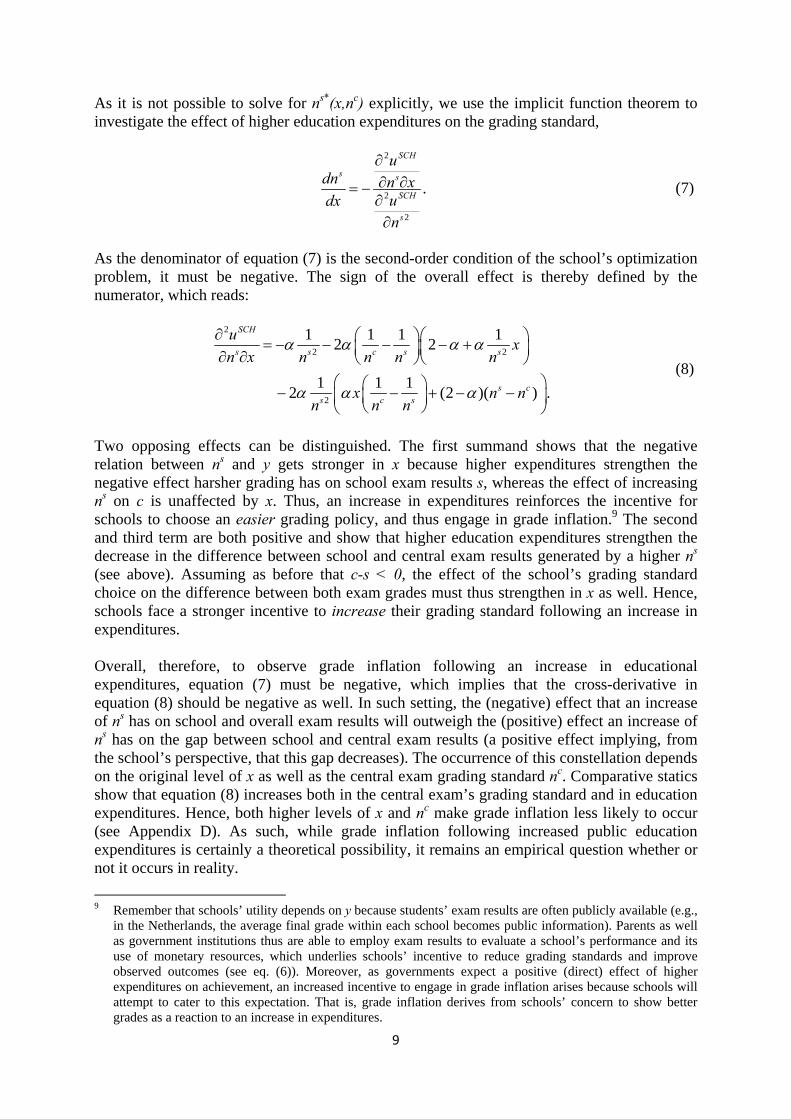
As it is not possible to solve for ns*(x,nc) explicitly, we use the implicit function theorem to investigate the effect of higher education expenditures on the grading standard,

2

2

2

.

SCH

s s

SCH

s

udn n x

udxn

(7)

As the denominator of equation (7) is the second-order condition of the school’s optimization problem, it must be negative. The sign of the overall effect is thereby defined by the numerator, which reads:

2

2 2

2

1 1 1 12 2

1 1 1 2 (2 )( ) .

SCH

s s c s s

s cs c s

ux

n x n n n n

x n nn n n

(8)

Two opposing effects can be distinguished. The first summand shows that the negative relation between ns and y gets stronger in x because higher expenditures strengthen the negative effect harsher grading has on school exam results s, whereas the effect of increasing ns on c is unaffected by x. Thus, an increase in expenditures reinforces the incentive for schools to choose an easier grading policy, and thus engage in grade inflation.9 The second and third term are both positive and show that higher education expenditures strengthen the decrease in the difference between school and central exam results generated by a higher ns (see above). Assuming as before that c-s < 0, the effect of the school’s grading standard choice on the difference between both exam grades must thus strengthen in x as well. Hence, schools face a stronger incentive to increase their grading standard following an increase in expenditures. Overall, therefore, to observe grade inflation following an increase in educational expenditures, equation (7) must be negative, which implies that the cross-derivative in equation (8) should be negative as well. In such setting, the (negative) effect that an increase of ns has on school and overall exam results will outweigh the (positive) effect an increase of ns has on the gap between school and central exam results (a positive effect implying, from the school’s perspective, that this gap decreases). The occurrence of this constellation depends on the original level of x as well as the central exam grading standard nc. Comparative statics show that equation (8) increases both in the central exam’s grading standard and in education expenditures. Hence, both higher levels of x and nc make grade inflation less likely to occur (see Appendix D). As such, while grade inflation following increased public education expenditures is certainly a theoretical possibility, it remains an empirical question whether or not it occurs in reality.

                                                            9 Remember that schools’ utility depends on y because students’ exam results are often publicly available (e.g.,

in the Netherlands, the average final grade within each school becomes public information). Parents as well as government institutions thus are able to employ exam results to evaluate a school’s performance and its use of monetary resources, which underlies schools’ incentive to reduce grading standards and improve observed outcomes (see eq. (6)). Moreover, as governments expect a positive (direct) effect of higher expenditures on achievement, an increased incentive to engage in grade inflation arises because schools will attempt to cater to this expectation. That is, grade inflation derives from schools’ concern to show better grades as a reaction to an increase in expenditures.

10 

 

3.4 Overall effect on attainment

We are now also in a position to assess the overall effect an expenditure change exerts on educational attainment (as extensively discussed in the foregoing literature). Indeed, using the above, equation (1) becomes:

2

1 1 1.

s s s

c s s s

dy e n e n ne x xe

dx n n n x x x n x

(9)

Equation (9) shows the direct effect of an expenditure change, its impact on school-level grading standards as well as the adjustment in student effort (caused by the change in x and the ensuing adjustment of the school’s grading policy). It indicates that the direct effect is unambiguously positive for both exams, whereas the students’ effort decrease (as a reaction to higher expenditures) has a negative impact. Moreover, when an expenditure increase leads to

grade inflation 0sn

x

, the lower level of ns will not only directly improve school exam

results, but also reduce student effort. As the latter effect deteriorates both school and central exam results, the direct and effort effects work in opposite directions at the school level, resulting in a negative overall impact (see section 3.3). In contrast, central exam results will

unambiguously fall as their difficulty does not vary in expenditures. For 0sn

x

, the signs of

these effects are reversed. The theoretical model thus allows us to derive the following predictions, which will be tested empirically in section 4. Hypothesis 1: An increase in educational spending changes the schools’ grading behavior. Hypothesis 2: If nS increases (decreases), results on the central exam improve (deteriorate), whereas results on the school-level exam deteriorate (improve). It is worth highlighting that by these various effects, our simple theoretical framework provides a possible explanation for the diversity of opinion in the empirical literature about the effects of increased educational spending (see section 2). Indeed, even when we start out by assuming that an increase in educational spending has a positive direct influence on student achievement, adjustments in students’ and schools’ behavior in response to changes in available resources may create important counteracting effects, and can reverse the overall impact. The existing literature disregards these behavioral effects. Accounting for such behavioral feedback effects, however, it becomes clear that the overall effect of resource-driven policies depends on the relative strength of the direct and indirect effects outlined above, which is likely to vary substantially across institutional contexts.

11 

 

4. Institutional setting and data

4.1. The outcome: School and central exit exams

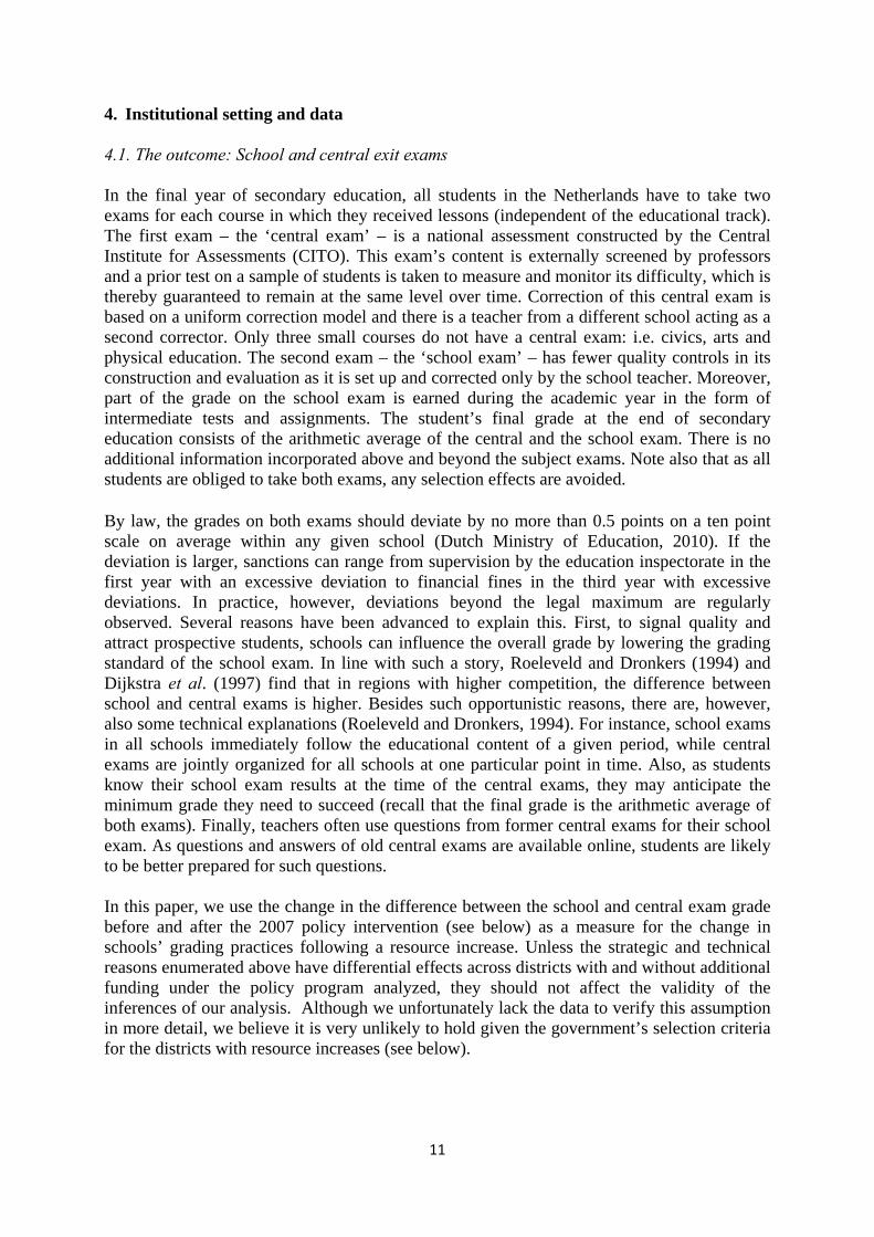
In the final year of secondary education, all students in the Netherlands have to take two exams for each course in which they received lessons (independent of the educational track). The first exam – the ‘central exam’ – is a national assessment constructed by the Central Institute for Assessments (CITO). This exam’s content is externally screened by professors and a prior test on a sample of students is taken to measure and monitor its difficulty, which is thereby guaranteed to remain at the same level over time. Correction of this central exam is based on a uniform correction model and there is a teacher from a different school acting as a second corrector. Only three small courses do not have a central exam: i.e. civics, arts and physical education. The second exam – the ‘school exam’ – has fewer quality controls in its construction and evaluation as it is set up and corrected only by the school teacher. Moreover, part of the grade on the school exam is earned during the academic year in the form of intermediate tests and assignments. The student’s final grade at the end of secondary education consists of the arithmetic average of the central and the school exam. There is no additional information incorporated above and beyond the subject exams. Note also that as all students are obliged to take both exams, any selection effects are avoided.  By law, the grades on both exams should deviate by no more than 0.5 points on a ten point scale on average within any given school (Dutch Ministry of Education, 2010). If the deviation is larger, sanctions can range from supervision by the education inspectorate in the first year with an excessive deviation to financial fines in the third year with excessive deviations. In practice, however, deviations beyond the legal maximum are regularly observed. Several reasons have been advanced to explain this. First, to signal quality and attract prospective students, schools can influence the overall grade by lowering the grading standard of the school exam. In line with such a story, Roeleveld and Dronkers (1994) and Dijkstra et al. (1997) find that in regions with higher competition, the difference between school and central exams is higher. Besides such opportunistic reasons, there are, however, also some technical explanations (Roeleveld and Dronkers, 1994). For instance, school exams in all schools immediately follow the educational content of a given period, while central exams are jointly organized for all schools at one particular point in time. Also, as students know their school exam results at the time of the central exams, they may anticipate the minimum grade they need to succeed (recall that the final grade is the arithmetic average of both exams). Finally, teachers often use questions from former central exams for their school exam. As questions and answers of old central exams are available online, students are likely to be better prepared for such questions. In this paper, we use the change in the difference between the school and central exam grade before and after the 2007 policy intervention (see below) as a measure for the change in schools’ grading practices following a resource increase. Unless the strategic and technical reasons enumerated above have differential effects across districts with and without additional funding under the policy program analyzed, they should not affect the validity of the inferences of our analysis. Although we unfortunately lack the data to verify this assumption in more detail, we believe it is very unlikely to hold given the government’s selection criteria for the districts with resource increases (see below).

12 

 

4.2. The intervention: Earmarked block grants in specific districts

As in most other Western countries, some neighborhoods in the Netherlands are characterized by a combination of poverty, unemployment and social instability. Such neighborhoods have recently been labeled as power districts (‘krachtwijken’ in Dutch). They are also known as ‘attention districts’ (‘aandachtswijken’ in Dutch) or ‘Vogelaar-areas’ (after the responsible minister). Shortly after its appointment on 22 February 2007, the Balkenende IV administration announced a new policy program aimed at addressing key social problems in a pre-specified number of such districts. Specifically, the Ministry of Housing selected 40 neighborhoods – consisting of 83 postcode areas situated in 18 large and medium-sized Dutch cities10 – to receive additional block grants earmarked to improve the social, physical and economic environment of these districts. The total subsidy for the 40 areas amounted to 250 million euro annually (ranging from €1.2 million to €29.3 million across districts, or €333 to €3995 per inhabitant in the districts), and the selection of the districts was driven by a set of 18 indicators including the income, education and unemployment levels within the local population, the incidence of public disorder issues (such as graffiti and vandalism), the average age and condition of the housing stock and the local population’s opinions regarding public safety in the area (Tweede Kamer, 2008-2009). The final decision to include or exclude districts was taken by the minister (i.e., Ella Vogelaar) roughly one month after the new government was inaugurated, and the program was announced and implemented in July 2007. Although the speed and organization of the selection process precluded extensive lobbying efforts by districts desiring to be included (thus mitigating concerns arising from potential self-selection), the selection process obviously was non-random since the government aimed at selecting the worst-performing districts. Fortunately, while schools in selected districts performed worse on our central outcome variables (i.e., exam grades), the pre-treatment trend in exam grades did not differ significantly across selected and unselected districts (see Table C1 in Appendix C). Moreover, the government selected only 40 districts, which left a substantial number of similarly ‘underperforming’ districts outside the chosen sample. As a result, we are left with a quasi-experimental setting where some underperforming districts were selected to receive additional funding while other underperforming districts received no such funding. This is exploited in the empirical analysis below. We should also note that while the various actors involved in the policy program (i.e., schools, local government, housing corporations and the regional government) retained some leeway in setting their objectives, schooling and youth received substantial attention across the board. For instance, in 16 out of the 18 cities with power districts, investments were explicitly aimed at improving the schooling outcomes of local youth. This makes the improvement of education the most central and commonly stated ambition in the power district policy (Tweede Kamer, 2008-2009, 68).11

                                                            10   The selection of postcode areas was based on a long-list with 180 additional postcode areas (which did not

receive additional funding). Information on the excluded postcodes has not been made public, and is considered ‘highly confidential’ by the Dutch government. 

11 Excluding both cities that did not explicitly mention education investments in their power districts policy program leaves our results unaffected (details upon request).

13 

 

4.3. The data

School-level data on student performance (i.e., our dependent variables) originate from the Dutch Ministry of Education. The variables of interest are the results on the central and school exams, where grades are collected on an average level across subjects within schools on an annual basis. Our dataset includes information for 738 schools, which are well spread across the Netherlands, over the period 2004-2009 (although previous years are available, they cannot be included due to data inconsistencies). Since estimation approaches based on a differences-in-differences (DiD) framework – as used below – yield inconsistent standard errors when the data consist of serially correlated outcomes, we follow the suggestion of Bertrand et al. (2004) and average exam results by school over the period before (i.e., 2004-2006) and following (i.e., 2008-2009) the intervention. This approach “works well even for small numbers [of observations]” (Bertrand et al., 2004, p. 249).12 For ease of interpretation, we recalibrate all grades into the 0-10 band. While we unfortunately lack information about, for instance, the number (or quality) of teachers and school provisions (such as the number of computer terminals, the presence/size of a school library, …), we do have information on the size of the student population in a subset (N=523) of schools. Besides information at the school level, we also observe postcode information for each school, such that we can match each school to data on socio-demographic characteristics in its neighborhood (obtained from Statistics Netherlands). This provides us with information on the number of inhabitants, urbanization (5-point scale with 1 urban and 5 rural), percentage of employed residents and welfare recipients (both as share of working-age population), average income (measured as after-tax income in 1000€) and the percentage of young (under 25), old (over 65) and immigrant citizens (all as a share of total population). Descriptive statistics are presented in Table 1. We thereby separate the data on exam results for the period before (2004-06) and after (2008-09) the policy intervention, but present background characteristics only for the post-intervention period. In line with previous observations (see above), the average grades on the central exit exam lie below those on the school exam. This holds both before and after the policy intervention, though the average difference between both types of exams increases over time (from 0.317 points to 0.492 points). This is largely driven by worsening central exam results (see, Dronkers, 2012, for a similar observation). Finally, it is important to note that the mean difference between both exam types hides significant heterogeneity across schools. We exploit this variation in the analysis below.

___________________

Table 1 about here

___________________

                                                            12 Note that we exclude the year of the intervention (i.e., 2007) from the analysis. We deem this most

appropriate even though exams for that year had already passed by the time of the intervention and thus could not possibly be influenced by it.

14 

 

5. Empirical analysis

5.1. Empirical Strategy

As mentioned, our estimation approach is based on a differences-in-differences (DiD) framework, in which we exploit the variation in public investment across space and time due to the July 2007 policy intervention. The existence of comparable neighborhoods without additional funding allows us to infer the counterfactual outcome and to estimate the causal impact of public resources. Particularly, we estimate the causal effect of the policy intervention on the grading by comparing educational outcomes in Dutch schools inside the 40 districts covered by the new legislation (the ‘treated’ group; 35 schools) with those not covered by the new legislation (the ‘control’ group; 703 schools) before/after 2007 using information covering the 2004-2009 period (albeit collapsed into a pre- and post-treatment period; see above). As such, the control group consists of all observed schools not located in one of the power districts.13 This leads to the following baseline specification (with subscript i referring to schools and subscript t to time):

SE_CEi,t = δ + PowerDistricti,t + Timet + PowerDistricti,t * Timet + k k Xi,t + i,t (10)

where SE_CEi,t reflects the difference at time t in the mean result of school i’s pupils on the school exams (SE) and the central exams (CE). Positive numbers indicate that a school’s pupils perform better on the school than the central exams (and vice versa). We also estimate the model separately for SE and CE as this yields an indication on the progress in educational attainment. δ indicates a school and time independent constant intercept. The variable PowerDistricti,t is an indicator variable equal to 1 for the districts receiving additional block grants, and 0 otherwise. Its estimated coefficient indicates the time and school invariant constant effect from the disadvantageous power districts. The indicator variable Timet captures the time fixed effect separating the period before (Timet=0; i.e., the 2004-2006 period) and after the policy intervention (Timet=1; i.e., the 2008-2009 period). The variable of interest is the interaction effect of Timet and PowerDistricti,t. It equals 1 for schools in a power district after 2007, and 0 otherwise. Its coefficient estimates the causal effect from the additional resources of the policy intervention on SE_CEi,t. Xi,t stands for a vector of (k=5) control variables including the district population size and the school’s student number (both in logarithmic form), the share of immigrant, young (i.e., under 25) and old (i.e., over 65) residents in the district population. While these five variables exhaust the information available,14 their inclusion may be critical to adjust for any differences in educational attainment that are a function of the population and student composition (Berrebi and Klor, 2008; Fiva, 2009) – especially when the government’s selection process may have been influenced by such observable socio-demographic indicators.15 Finally, i,t denotes an error term with zero mean and constant variance.

                                                            13 As the similarity of the treated and control groups is critical, we return to the specification of the control

group in more detail when discussing our results. 14 The information on urbanization, employment, income and the share of welfare recipients mentioned above

is only available for the year 2003, and thus cannot be included in our fixed effects estimation (see below). We do, however, use this information in our robustness checks based on a matching estimator.

15 Auxiliary regressions indicate that especially the share of immigrants in the district’s population appears strongly positively correlated with both selection into, and the size of the additional funding provided within, the policy program (details available upon request) – highlighting the importance of directly controlling for this factor.

15 

 

Given the non-random selection of the power districts, schools in the power districts might be different from schools in other areas. To accommodate this, we extend equation (10) with school-specific (i) fixed effects that capture all time-invariant differences across schools. As these fixed effects are perfectly collinear with PowerDistricti,t, we remove the latter to obtain the following model:

SE_CEi,t = i + Timet + PowerDistricti,t * Timet + k k Xi,t + i,t, (11)

where remains the variable of interest with a similar interpretation as above. Including school fixed effects comes at the cost of not being able to report an estimate of the PowerDistricti,t variable. The benefit, however, is that school-specific fixed effects allow us to control for unobserved heterogeneity across schools – also among schools within the power districts. This is critical to obtain valid inferences. Hence, below, we only present results for the fixed effects model (i.e., equation 11). Still, by relying on an indicator variable to distinguish treated and untreated districts, this baseline approach ignores the variation in the intensity of the treatment across power districts (see above). Therefore, we extend the empirical model by explicitly including the level of additional public spending created by the new legislation. Hence, unlike the traditional DiD approach, we exploit this information for identification purposes by “relying on an explanatory variable with differing treatment intensity across localities” (Berrebi and Klor, 2008, p. 208; Angrist and Pischke, 2008). This extends our estimation equation in the following way:

SE_CEi,t = i + Timet + PowerDistricti,t * Timet + 4 Investmenti,t + k k Xi,t + i,t (12)

where Investmenti,t equals the level of annual additional public investment (in million €) in district i at time t deriving from the new policy program. Clearly, this is 0 before the intervention, but varies across districts after the intervention (though remaining 0 in ‘untreated’ districts). Investmenti,t equals the total additional investment in the neighborhood, although taking instead the investment level per inhabitant in the district leaves our results qualitatively unaffected (details upon request). The inclusion of the investment level along with the indicator variable for being located in a power district permits disentangling the effect of receiving the status as ‘Power district’ at time t (3) from the effect of the public expenditures associated with this status (4). The key identifying assumption underlying equations (10) through (12) is that the trends in educational outcomes in treated and untreated districts would be the same except for the intervention (the parallel time trend assumption; Bertrand et al., 2004; Webbink, 2007). This raises two issues. First, as mentioned, the government selected worst-performing districts non-randomly.16 Selection of worst-performing districts implies that the trend in treated

                                                            16 Such selection appears to have been successful. Auxiliary regressions illustrate that the average grade on

central exams in the pre-treatment period rises strongly and significantly with the distance from the selected districts. Exam results are worst when distance is 0; i.e., for the selected districts. Similarly, the level of additional funding within the policy program is significantly negatively related to performance on the central exam (details available upon request).

16 

 

districts may, if anything, have been more negative prior to the intervention. This, however, is unproblematic from our perspective as it would work against finding a positive effect from the policy program in our estimations (making our estimation results reflect a lower bound of the true effect).17 Moreover, auxiliary regressions indicate no evidence that the downward pre-treatment trend in central exam grades (also observed in Dronkers, 2012) is different for our treatment and control groups (see Table C1 in Appendix C). Second, migration flows triggered by the policy intervention may lead to violations of the parallel time trend assumption. In this respect, it is important to note that the list of selected districts was only made publicly available after a lengthy legal proceeding in February 2009. Consequently, any in- or outward mobility between July 2007 and (at least) February 2009 can reasonably be taken as independent of residents’ district being included in the list. This is important as students in the Netherlands have a fully free school choice (there is no catchment area). Even so, data from Statistics Netherlands illustrate that the share of western migrants, non-western migrants, natives, people below the age of 20, citizens above 65 years, employed, unemployed and one-parent-families is stable over time in both treated and untreated districts (i.e., the share of these respective population groups does not change significantly over the 2004-2009 period). This strongly suggests that there were no obvious changes in the underlying population in the 2004-2009 period. 5.2. Empirical Results

Our baseline findings, which exploit the full set of 738 available schools, are summarized in Table 2. Still, given the importance of appropriately circumscribing the control group, section 5.3 below will report on a number of robustness checks with different (and more restrictive) control groups. In Table 2, columns (1) through (3) provide results for the estimation of equation (11). Columns (4) through (6) also include the annual investment level due to the policy program within every district. In each case, the first column (i.e., column (1) and (4)) has as dependent variable the difference between school and central exam results, while the next two columns have, respectively, school and central exam results as their dependent variable. By estimating specifications with all three dependent variables, we can evaluate Hypothesis 1 on the presence/absence of grade inflation from columns (1) and (4), while columns (2), (3), (5) and (6) provide the testing ground for Hypothesis 2.

___________________

Table 2 about here

___________________

The results in Table 2 indicate that when looking at the policy intervention using an indicator variable (columns (1) through (3)), our evidence concerning Hypotheses 1 and 2 is relatively weak. No statistically significant effects are obtained from additional resources on either school (column (2)) or central exams (column (3)): i.e., the interaction effects in columns (2) and (3) remain statistically insignificant at conventional levels. Although one explanation may lie in the fact that we evaluate the policy intervention immediately after the investments

                                                            17 If improvements take some time to fully develop and become visible in exam grades, the fact that we study a

time-period immediately after the policy intervention may exert some additional downward pressure on our coefficient estimates for both exam results. This should not, however, undermine our ability to detect (potential) adjustments in school-level grading practices.

17 

 

started (see above), the direction of both effects – cautiously interpreted – does tell us something. From the theoretical model, we indeed know that this pattern – i.e. the negative coefficient in column (3) and the positive coefficient in column (2) – is suggestive of some degree of grade inflation due to schools reducing the school-level grading standard (nS) (see Hypothesis 2). This is also reflected in column (1). Although the effect is once again relatively weak (p=0.112), given the time span and the estimation of lower bound estimates it provides a first indication that the (general) inability to immediately move grades to a higher level following improved resources may translate into a pressure to adjust grading structures to suggest an (unrealized) improvement (cf. Hypothesis 1). Columns (4) through (6) further explore the effect of the selective resource increase deriving from the policy program by adding the treatment intensity (as in equation (12)). This shows that the level of the additional investment plays a critical mediating role. Indeed, higher investment significantly dampens the relative decline in central exam results that is observed in power districts with ‘no’ additional funding (column (6)). This also becomes clear when illustrating the marginal effect of additional investments over the range of such investments observed in our sample in Figure 1c. Being designated as a power district has a statistically significant negative effect on central exam results until the investment surpasses approximately €11 million (or circa €1250 per resident), but has no significant effect for higher levels of investment. Although the effect of the additional investment on central exam results becomes positive around €17 million (or just over €2000 per resident), this fails to reach statistical significance at conventional levels within the range of spending observed in our sample. Once again, no significant effects are found for school-level exam results (column (5) and Figure 1b). Both results taken together suggest that the policy intervention worked to halt falling central exam results in the selected districts when additional funds were sufficiently elevated, but induced grade inflation when such funds were limited. Figure 1a illustrates that significant grade inflation is observed until the additional investment exceeds €12.5 million (or circa €1500 per resident).

___________________

Figure 1 about here

___________________

Although these results are robust to alternative specifications (see below), we regrettably cannot provide much detail about the underlying mechanism(s). One particularly interesting possibility may be that schools in districts receiving less funding might have used these resources for more basic investments (e.g., sport facilities, library expansion, computer or media rooms) that predominantly have an impact i) in the long run (but unobservable within the short period analysed), ii) on students’ behaviour/civic attitude (which affect teachers’ perceptions of students, and thereby their school-level grades), and iii) on topics not covered by the central test (i.e. civics, sport, art). While the first two of these effects can be categorized as specific forms of grade inflation – as school test results would not reflect students’ real, current academic performance – the latter cannot. Unfortunately, the lack of detailed spending data prevents us from investigating this issue in more detail.

18 

 

5.3. Robustness Checks

While the results in Table 2 remain robust when excluding the number of students from the set of control variables (which has a substantial number of missing observations, see Table 1) or using annual additional investments in per capita terms (as indicated between brackets in the discussion above), we also ran a number of checks on the selection of the control group. The first of these rests simply replicates all estimations in Table 2 restricting the sample to schools in districts that are very similar to the 40 treated districts in some socio-demographic dimension. Specifically, as treated districts where larger, younger and ethnically more diverse than untreated districts, we successively restricted the sample to schools in districts with at least as many inhabitants, young citizens or migrants, and at most the number of older citizens than the 40 treated districts. As can be seen from Table 3, none of these restrictions changes the inferences from those reported in Table 2. The same holds also when we impose all four restrictions at the same time to obtain the most restrictive control group feasible. Secondly, we implemented a matching estimator (using psmatch2 in Stata12; Leuven and Sianesi, 2010) because this a) exploits the purposeful assignment to the treatment and b) allows us to incorporate some additional background characteristics of the districts that do not change over time (see above). Using the results predicting treatment in the matching procedure18 to trim the sample based on the schools’ propensity scores leaves our results unaffected (see Table 4). Note also that the results from a standard matching estimator are consistent with the findings reported above (details provided in Appendix B).

___________________

Tables 3 and 4 about here

___________________

Finally, although the Dutch government did not aim to select districts that had been improving prior to 2007 (rather the reverse was intended), a last robustness check evaluates whether the results in Table 2 are really due to the 2007 policy intervention by implementing a placebo estimation comparing the 2004-05 period to the 2006-07 period. Given that no intervention had yet taken place, nor additional investments been made, in the 40 selected districts prior to July 2007 (when exams for the 2007 school year were already finished), no significant effects should arise in this exercise. As can be seen in the three left-hand side columns of Table 5, this is borne out since none of the coefficients of interest reaches statistical significance at conventional levels. We should note here that this is not due to the reduction in sample size (to 635 rather than 738 schools). In fact, running the original model (i.e., comparing the actual pre- and post-treatment periods) on this reduced sample once again produces significant effects very much in line with those reported in Table 2 (see right-hand side columns of Table 5).

                                                            18 To match treated and untreated districts, we ran a probit regression using population size, percentage

immigrants, the level of urbanization, the percentage of employed residents and welfare recipients (both as share of working-age population) and average income in the district (measured as after-tax income in 1000€) as explanatory variables. We also include squared terms of the share of immigrants and income to satisfy the balancing properties of the matching procedure. Including these variables, there remain no significant differences between the matched set of ‘treated’ and ‘untreated’ districts (details upon request).

19 

 

___________________

Table 5 about here

___________________

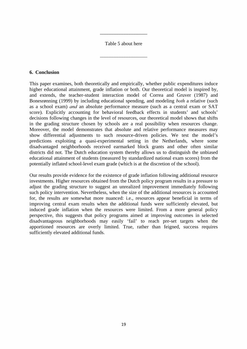
6. Conclusion

This paper examines, both theoretically and empirically, whether public expenditures induce higher educational attainment, grade inflation or both. Our theoretical model is inspired by, and extends, the teacher-student interaction model of Correa and Gruver (1987) and Bonesrønning (1999) by including educational spending, and modeling both a relative (such as a school exam) and an absolute performance measure (such as a central exam or SAT score). Explicitly accounting for behavioral feedback effects in students’ and schools’ decisions following changes in the level of resources, our theoretical model shows that shifts in the grading structure chosen by schools are a real possibility when resources change. Moreover, the model demonstrates that absolute and relative performance measures may show differential adjustments to such resource-driven policies. We test the model’s predictions exploiting a quasi-experimental setting in the Netherlands, where some disadvantaged neighborhoods received earmarked block grants and other often similar districts did not. The Dutch education system thereby allows us to distinguish the unbiased educational attainment of students (measured by standardized national exam scores) from the potentially inflated school-level exam grade (which is at the discretion of the school). Our results provide evidence for the existence of grade inflation following additional resource investments. Higher resources obtained from the Dutch policy program results in a pressure to adjust the grading structure to suggest an unrealized improvement immediately following such policy intervention. Nevertheless, when the size of the additional resources is accounted for, the results are somewhat more nuanced: i.e., resources appear beneficial in terms of improving central exam results when the additional funds were sufficiently elevated, but induced grade inflation when the resources were limited. From a more general policy perspective, this suggests that policy programs aimed at improving outcomes in selected disadvantageous neighborhoods may easily ‘fail’ to reach pre-set targets when the apportioned resources are overly limited. True, rather than feigned, success requires sufficiently elevated additional funds.

20 

 

References

Angrist, J.D. and J. Pischke (2008). Mostly Harmless Econometrics: An Empiricist’s Companion. Princeton: Princeton University Press.

Angrist, J.D. and V. Lavy (1999). Using Maimonides’ Rule to Estimate the Effect of Class Size on Scholastic Achievement. Quarterly Journal of Economics, 114(2): 533-575.

Backes-Gellner, U. and S. Veen (2008). The Consequences of Central Examinations on Educational Quality Standards and Labour Market Outcomes. Oxford Review of Education, 34(5): 569-588.

Berrebi, C. and E.F. Klor (2008). Are Voters Sensitive to Terrorism? Direct Evidence from the Israeli Electorate, American Political Science Review, 102(3): 279-301.

Bertrand, M., E. Duflo and S. Mullainathan (2004). How much should we trust Difference-in-Differences Estimates? Quarterly Journal of Economics 119(1): 249-275.

Betts, J.R. (1998). The Impact of Educational Standards on the Level and Distribution of Earnings. American Economic Review, 88(1): 266-275.

Bishop, J.H. (1999a). Are National Exit Examinations Important for Educational Efficiency? Swedish Economic Policy Review 6(2): 349-398.

Bishop, J.H. and L. Wößmann (2004). Institutional Effects in a Simple Model of Educational Production. Education Economics, 12(1): 17-38.

Bonesrønning, H. (1999). The Variation in Teachers’ Grading Practices: Causes and Consequences. Economics of Education Review, 18: 89-105.

Bonesrønning, H. (2004). Do the Teachers’ Grading Practices Affect Student Achievement? Education Economics, 12: 151-167.

Carnoy, M. and S. Loeb (2002). Does External Accountability Affect Student Outcomes? A Cross-State Analysis. Educational Evaluation and Policy Analysis, 24(4): 305-331.

Case, A. and A. Deaton (1999). School Inputs and Educational Outcomes in South Africa. Quarterly Journal of Economics, 114(3): 1047-1084.

Correa, H. and G.W. Gruver (1987). Teacher-Student Interaction: A Game-Theoretic Extension of the Economic Theory of Education. Mathematical Social Sciences, 13: 19-47.

Das, J., Dercon, S., Habyarimana, J., Krishnan, P., Muralidharan, K. and Sundararaman, V. (2012). School Inputs, Household Substitution, and Test Scores, American Economic Journal: Applied Economics, forthcoming.

DePaola, M. and V. Scoppa (2007). Returns to Skills, Incentives to Study and Optimal Educational Standards. Journal of Economics, 92(3): 229-262.

DePaola, M. and V. Scoppa (2010). A Signalling Model of School Grades under Different Evaluation Systems. Journal of Economics, 101: 199-212.

Dijkstra, A. B., J. Dronkers and R.H. Hofman (1997). Verzuiling in het onderwijs. Actuele verklaringen en analyse. Groningen: Wolters-Noordhoff.

De Witte, K. and Van Klaveren, C. (2012), Comparing Students by a Matching Analysis – On Early School Leaving in Dutch Cities. Applied Economics 44 (28), 3679-3690.

Dronkers, J. (2012). SE-CE verschillen per vak en VWO- en HAVO-locatie. Algemene Onderwijsbond. Utrecht.

21 

 

Dutch Ministry of Education (2010). Examenlicentie kwijt bij grote verschillen examencijfers. Persbericht 25-06-2010.

Figlio, D.N. and M.E. Lucas (2004). Do High Grading Standards affect Student Performance? Journal of Public Economics, 88: 1815-1834.

Fiva, J.H. (2009). Does Welfare Policy Affect Residential Choices? An Empirical Investigation Accounting for Policy Endogeneity, Journal of Public Economics, 93: 529-540.

Gerritsen, S. and D. Webbink (2010). The Effects of Extra Funds for 40 Disadvantaged Neighborhoods. Paper presented at a Centraal Planbureau Conference at Rijksuniversiteit Groningen, March 3, 2010.

Hanushek, E.A. (2003). The Failure of Input-Based Schooling Policies. Economic Journal, 113(February): F64-F98.

Hanushek, E.A. and D.D. Kimko (2000). Schooling, Labor-Force Quality, and the Growth of Nations. American Economic Review, 90(5): 1184-1208.

Himmler, O. and R. Schwager (2012). Double Standards in Educational Standards - Are Disadvantaged Students Being Graded More Leniently? German Economic Review, forthcoming.

Holmlund, H., S. McNally and M. Viarengo (2010). Does Money Matter for Schools? Economics of Education Review, 29(6): 1154-1164.

Houtenville, A.J. and K.S. Conway (2008). Parental Effort, School Resources, and Student Achievement. Journal of Human Resources, 43(2): 437-453.

Hoxby, C.M. (2000). The Effects of Class Size on Student Achievement: New Evidence from Population Variation. Quarterly Journal of Economics, 115(4): 1239-1285.

Jacob, B.A. (2005). Accountability, Incentives and Behavior: The Impact of High-Stakes Testing in the Chicago Public Schools. Journal of Public Economics, 89: 761-796.

Jacob, B.A. and S.D. Levitt (2003). Rotten Apples: An Investigation of the Prevalence and Predictors of Teacher Cheating. Quarterly Journal of Economics, 118(3): 843-877.

Koning, P. and K. van der Wiel (2012). School Responsiveness to Quality Rankings: An Empirical Analysis of Secondary Education in the Netherlands. De Economist, 160(4): 339-355.

Koning, P. and K. van der Wiel (2013). Ranking the Schools: How School-Quality Information Affects School Choice in the Netherlands, Journal of the European Economic Association, forthcoming.

Krueger, A.B. (1999). Experimental Estimates of Education Production Functions. Quarterly Journal of Economics, 114: 497-532.

Krueger, A.B. and D.M. Whitmore (2001). The Effect of Attending a Small Class in the Early Grades on College-Test Taking and Middle School Test Results: Evidence from Project STAR. Economic Journal, 111: 1-28.

Lee, J. and R.J. Barro (2001). Schooling Quality in a Cross-section of Countries. Economica, 68: 465-488.

Leuven, E. and B. Sianesi (2010). PSMATCH2: Stata Module to Perform Full Mahalanobis and Propensity Score Matching, Common Support Graphing, and Covariate Imbalance Testing (version 4.0.4.). http://ideas.repec.org/c/boc/bocode/s432001.html.

22 

 

Martins, P.S. (2009). Individual Teacher Incentives, Student Achievement and Grade Inflation. IZA Discussion Paper Series nr. 4051.

Neal, D. and D. Whitmore Schanzenbach (2010). Left Behind by Design: Proficiency Counts and Test-Based Accountability. Review of Economics and Statistics, 92(2): 263-283.

Rajkumar, A.S. and V. Swaroop (2008). Public Spending and Outcomes: Does Governance Matter? Journal of Development Economics, 86(11): 96-111.

Reback, R. (2008). Teaching to the Rating: School Accountability and the Distribution of Student Achievement. Journal of Public Economics, 92: 1394-1415.

Rockoff, J.E. and L.J. Turner (2010). Short Run Impacts of Accountability on School Quality. American Economic Journal: Economic Policy, 2(4): 119-147.

Roeleveld, J. and J. Dronkers (1994), Bijzondere of buitengewone scholen? Verschillen in effectiviteit van openbare en confessionele scholen in regio's waarin hun richting een meerderheids- of minderheidspositie inneemt, Mens en Maatschappij, 69, 85-108.

Tweede Kamer (2008-2009). Krachtwijken: Monitoring en verantwoording van het beleid, Tweede Kamer der Staten-Generaal, 31.723, nr. 1-2, ‘s Gravenhage.

Wikström, C. and M. Wikström (2005). Grade Inflation and School Competition: An Empirical Analysis based on the Swedish Upper Secondary Schools, Economics of Education Review, 24(3): 309-322.

Wittebrood, K. and M. Permentier (2011). Wonen, wijken en interventies: Krachtwijkenbeleid in perspectief, Sociaal en Cultureel Planbureau.

Wößmann, L. (2003). Schooling Resources, Educational Institutions, and Student Performance: the International Evidence. Oxford Bulletin in Economics and Statistics, 65(2): 117-170.

Walsh, J. (1979). Does High School Grade Inflation Mask a More Alarming Trend? Science 203(4384): 982.

Webbink, D. (2007). Return to University Education: Evidence from a Dutch Institutional Reform, Economica, 74: 113-134.

Wolf, A. (2004). Does Education Matter? Penguin Books Ltd., London.

23 

 

Table 1: Descriptive statistics (N=738)

Min Quartile 1 Median Mean Quartile 3 Max Central exam (pre-intervention: 2004-06) 4.520 5.716 6.550 6.414 7.070 8.914 School exam (pre-intervention: 2004-06) 5.850 6.409 6.683 6.732 6.991 8.563 Diff central & school exam (pre-intervention: 2004-06) -1.612 -0.694 -0.038 0.317 1.267 3.373 Central exam (post-intervention: 2008-09) 4.236 5.590 6.301 6.236 6.867 8.936 School exam (post-intervention: 2008-09) 5.824 6.378 6.656 6.728 6.994 8.700 Diff central & school exam (post-intervention: 2008-09) -1.337 -0.506 0.169 0.492 1.416 3.539 Subsidy (million €) 0.000 0.000 0.000 0.556 0.000 29.300Total population 295 5566 8020 8046.484 10670 20570 Total number of students a 35 431 770 874.941 1256 2603 Income (in 1000€) 9.150 12.000 13.082 13.589 14.400 25.600Share employed 39.000 65.000 69.333 68.729 73.000 85.000Share welfare recipients 6.000 12.100 15.000 16.239 19.000 42.400Urbaneness (5-point scale) 1.000 1.800 2.739 2.808 4.000 5.000 Immigrant population 0.027 0.118 0.186 0.209 0.266 0.861 Share younger than 25 0.012 0.097 0.115 0.113 0.128 0.202 Share older than 65 0.015 0.131 0.169 0.172 0.207 0.488 Note: a We only observe the total number of students for 523 schools.

24 

 

Table 2: Regression results using full sample (N=738 schools)

  Results of equation (11) Results of equation (12)   (1)

SE_CE (2) SE

(3) CE

(4) SE_CE

(5) SE

(6) CE

Power district * 

Time () 0.133 (1.59)

0.042 (0.90)

-0.091 (-1.15)

0.413 *** (2.97)

0.069 (0.89)

-0.344 *** (-2.60)

Investment  

(mio €; 4) 

- - - -0.022 ** (-2.51)

-0.002 (-0.44)

0.019 ** (2.38)

Period 2  

(yes = 1; ) 0.172 ***

(9.15) -0.015 (-1.47)

-0.187 *** (-10.52)

0.172 *** (9.23)

-0.015 (-1.47)

-0.188 *** (-10.60)

Population (log)  0.565 (1.05)

0.260 (0.87)

-0.305 (-0.60)

0.545 (1.02)

0.258 (0.86)

-0.287 (-0.57)

Students (log)  0.936 (1.51)

0.445 (1.28)

-0.491 (-0.83)

0.873 (1.41)

0.438 (1.26)

-0.434 (-0.74)

Students2 (log)  -0.072 (-1.46)

-0.030 (-1.10)

0.042 (0.89)

-0.069 (-1.41)

-0.030 (-1.09)

0.039 (0.84)

Immigrants (%)  12.227 ** (2.44)

4.531 (1.62)

-7.696 (-1.62)

11.971 ** (2.40)

4.506 (1.61)

-7.464 (-1.57)

Immigrants2 (%)  -13.909 * (-1.79)

-5.989 (-1.38)

7.979 (1.07)

-13.669 * (-1.77)

-5.966 (-1.37)

7.703 (1.05)

Young (%)  -1.987 (-0.56)

-4.129 ** (-2.07)

-2.141 (-0.63)

-1.792 (-0.50)

-4.110 ** (-2.06)

-2.319 (-0.69)

Old (%)  -0.260 (-0.10)

-1.061 (-0.73)

-0.801 (-0.32)

-0.051 (-0.02)

-1.041 (-0.72)

-0.989 (-0.40)

  Fixed effects (i)  Yes Yes Yes Yes Yes Yes

 F (joint sign) 

11.99 ***

1.64 *

14.54 ***

11.53 ***

1.49

13.78 ***

Note: t-statistics in brackets; ***, **, * significant at 1%, 5% and 10%, respectively.

25  

Table 3: Regression results using restricted samples based on population characteristics

  SE_CE  SE  CE  SE_CE  SE  CE  SE_CE  SE  CE  SE_CE  SE  CE   Restricted migrant share  Restricted population size  Restricted young population  Restricted elderly population Power district 

* Time () 0.300 * (1.92) 

0.098 (1.11) 

‐0.202 (‐1.56) 

0.319 ** (1.97) 

0.074 (1.02) 

‐0.245 * (‐1.88) 

0.368 ** (2.54) 

0.108 (1.54) 

‐0.261 ** (‐2.12) 

0.359 ** (2.30) 

0.091 (1.26) 

‐0.267 ** (‐2.08) 

Investment  

(mio €; 4) 

‐0.021 ** (‐2.08) 

‐0.003 (‐0.56) 

0.018 ** (2.12) 

‐0.020 * (‐1.86) 

‐0.004 (‐0.89) 

0.016 * (1.81) 

‐0.022 **(‐2.28) 

‐0.005 (‐1.14) 

0.017 ** (2.04) 

‐0.022 **(‐2.10) 

‐0.005 (‐1.03) 

0.017 ** (1.96) 

Period 2  

(yes = 1; ) 0.182 *** (3.81) 

‐0.044 (‐1.62) 

‐0.225 *** (‐5.70) 

0.180 *** (7.90) 

‐0.003 (‐0.33) 

‐0.183 *** (‐9.97) 

0.163 *** (6.94) 

‐0.019 * (‐1.68) 

‐0.182 *** (‐9.11) 

0.164 *** (7.03) 

‐0.009 (‐0.79) 

‐0.172 *** (‐8.94) 

 N F (joint sign) 

 163 

4.75 *** 

 163 1.84* 

 163 

7.14 *** 

 674 

9.43 *** 

 674 1.01 

 674 

14.30 *** 

 539 

8.23 *** 

 539 1.20 

 539 

12.85 *** 

 612 

8.08 *** 

 612 0.57 

 612 

12.53 *** Note: Controls included as in table 2 (except for Students, which is excluded here to maintain sufficient sample sizes). t-statistics in brackets; ***, **, * significant at 1%, 5% and 10%, respectively.

26  

Table 4: Regression results using restricted samples based on propensity scores

  SE_CE  SE  CE  SE_CE  SE  CE  SE_CE  SE  CE   Excluding propensity scores  

<1% and >99% Excluding propensity scores  

<5% and >95% Excluding propensity scores  

<10% and >90% Power district * 

Time () 0.358 ** (2.27) 

0.103 (1.32) 

‐0.254 ** (‐2.00) 

0.419 ** (2.32) 

0.090 (0.98) 

‐0.330 ** (‐2.40) 

0.482 ** (2.13) 

0.160 (1.44) 

‐0.321 * (‐1.91) 

Investment  

(mio €; 4) 

‐0.022 ** (‐2.30) 

‐0.004 (‐0.76) 

0.019 ** (2.40) 

‐0.026 ** (‐2.38) 

‐0.003 (‐0.51) 

0.023 *** (2.79) 

‐0.027 ** (‐2.12) 

‐0.002 (‐0.36) 

0.025 ** (2.61) 

Period 2  

(yes = 1; ) 0.164 *** (2.66) 

‐0.039 (‐1.28) 

‐0.203 *** (‐4.11) 

0.151 * (1.80) 

‐0.030 (‐0.72) 

‐0.181 *** (‐2.84) 

0.071 (0.67) 

‐0.071 (‐1.35) 

‐0.141 * (‐1.79) 

 N F (joint sign) 

 200 

3.35 *** 

 200 0.83 

 200 

5.16 *** 

 138 

2.72 *** 

 138 0.52 

 138 

4.39 *** 

 104 1.66 

 104 0.76 

 104 

2.46 ** Note: Controls included as in table 2 (except for Students, which is excluded here to maintain sufficient sample sizes). t-statistics in brackets; ***,

**, * significant at 1%, 5% and 10%, respectively. Propensity scores obtained from a probit regression using population size and percentage immigrants (and its squared value) as well as the level of urbanization, the percentage of employed residents and welfare recipients (both as share of working-age population) and average income in the district (measured as after-tax income in 1000€; and its squared value) as explanatory variables.

27  

Table 5: Regression results of placebo estimation (2004-05, 2006-07)

  SE_CE  SE  CE  SE_CE  SE  CE   Comparing 2004‐05 to 2006‐07  

(placebo) Comparing 2004‐06 to 2008‐09  

(treatment) Power district * 

Time () 0.168 (1.22) 

0.103 (0.78) 

‐0.064 (‐0.34) 

0.448 *** (2.92) 

0.086 (1.00) 

‐0.361 ** (‐2.47) 

Investment  

(mio €; 4) 

‐0.010 (‐1.27) 

‐0.004 (‐0.48) 

0.007 (0.59) 

‐0.021 ** (‐2.24) 

‐0.003 (‐0.61) 

0.018 ** (1.99) 

Period 2  

(yes = 1; ) 0.178 *** (10.12) 

‐0.063 *** (‐3.77) 

‐0.241 *** (‐9.84) 

0.173 *** (8.74) 

‐0.017 (‐1.50) 

‐0.190 *** (‐10.04) 

 N F (joint sign) 

 635 

12.21 *** 

 635 

3.68 *** 

 635 

12.02 *** 

 636 

10.83 *** 

 636 1.61 

 636 

12.66 *** Note: Controls included as in table 2. t-statistics in brackets; ***, **, * significant at 1%, 5% and 10%, respectively.

28  

Figure 1: Marginal effect of additional investment on SE_CE (a), SE (b) and CE (c) -.4

-.20

.2.4

.6M

argi

nal E

ffect

of I

nves

tmen

t on

SE_C

E

0 5 10 15 20 25 30

Million

90% Confidence Interval

-.2-.1

0.1

.2

Mar

gina

l Effe

ct o

f Inv

estm

ent o

n S

E

0 5 10 15 20 25 30

Million

90% Confidence Interval

-.6-.4

-.20

.2.4

Mar

gina

l Effe

ct o

f Inv

estm

ent o

n C

E

0 5 10 15 20 25 30

Million

90% Confidence Interval

a) SE_CE

b) SE

c) CE

29  

Appendix A: Alternative specification of the exam result function

Apart from the setting presented in the main text, we consider a second possibility to model the functional form of the function describing the overall exam results:

( , )

( , , )

11 .

c e x

s e x n

y xe xen

   (13) 

Again, both the central and the school exam results can be influenced by the students’ effort

choice. Different from before is that students now receive 1

n points on the school exam that

may result from knowing the kind of questions the teacher might ask (remember that teachers appear to recycle central exam questions in school exams; Roeleveld and Dronkers, 1994). Alternatively, it can be interpreted as reflecting the lower average difficulty of school exams (compared to central exams). The students’ maximization problem in equation (2) then gives the following results:

*

*

2

*

2

1,

(1 )

10 and

(1 )

10.

(1 )

ex n

e

n x n

e

x x n

The main difference in results from those presented in the main text is that a change in education expenditures now has a positive effect on student effort. Apart from that, the effects in the first-order condition are qualitatively similar as above. The school’s first-order condition for the optimal grading standard and the cross-derivative with respect to x now become:

* **

2 2

* ** * *

2 2

1 1 1

1 1 1 1 1 2

SCHdu e ex xe x

dn n n n n n

e exe xe x xe x

n n n n n n n

                        (14)

and

2

2 2 2

1 1 1 1 12 1 1

(1 ) (1 )

1 1 1 1 2 1 1 .

1

SCHux

n x n n n n n x n

xn n n n

(15)

30  

It is easy to see that the effects in equations (14) and (15) are qualitatively similar to the ones in equations (6) and (8) presented in the main text. An increase of n leads to better results in the central exam but lowers students’ grades in the school exam. The difference between the results decreases in the grading standard (if n < 1 is assumed, which is equivalent to the assumption of nc > ns from above). Higher educational spending strengthens the negative effect tougher grading has on school exam results, but also leads to a larger decrease in the results’ difference. Again, the overall effect is dependent on the relative strength of both effects, but, as before, grade inflation following increased public education expenditures remains a theoretical possibility.

31  

Appendix B: A matching approach

As an alternative to the difference-in-differences approach implemented in the main text, we replicated our analysis using a propensity-score matching estimator (using psmatch2 in Stata12; Leuven and Sianesi, 2010). While this alternative is quite restrictive in not permitting more than a binary treatment variable, nor an explicit modeling of the temporal shock induced by the policy intervention, it has the benefit of closely linking treated and untreated districts in the analysis (see also Wittebrood and Permentier, 2001; De Witte and Van Klaveren, 2012). As such, it can provide additional insights into the differences between a matched sample of treated and untreated districts before and after the policy intervention. After matching treated and untreated districts, we evaluate the average treatment effect on the treated and untreated both before (when schools in treated districts can be expected to have lower central exam results due to the government’s selection strategy) and after the policy intervention (when we should find significant treatment effects). The results are presented in Table B1. Note that we bootstrapped the estimated standard errors (with 5000 replications) to account for the fact that propensity scores are estimated. Table B1: Results from matching estimator (N=722 schools)   (1) 

SE_CE (2) SE 

(3) CE 

(10) SE_CE 

(11) SE 

(6) CE 

  BEFORE treatment  AFTER treatment Average Treatment Effect on Treated (ATT) 

0.294  6.530  6.236  0.557  6.549  5.992 

Average Treatment Effect on Matched Controls (ATC) 

‐0.255  6.434  6.689  ‐0.091  6.179  6.271 

Difference (ATT – ATC)  0.549 *  0.095  ‐0.453 *  0.648 **  0.370 **  ‐0.279 

Note: significance levels using bootstrapped standard errors; ***, **, * significant at 1%, 5% and 10%. Column (3) in Table B1 illustrates that the government indeed selected the worst-performing districts for additional funding. Compared to similar districts, schools in the 40 selected districts performed significantly worse prior to the policy intervention. Still, as there are no significant differences between both groups on the school grades (column (2)), this also reflects in substantially ‘inflated’ grades in the selected districts. Turning to the post-treatment period, the difference between central exam results in both sets of schools is no longer statistically significant (column (6)), but the school exam grades in treated schools are now significantly more elevated (column (5)). This is driven by the fact that central exam results fall approximately 40% less in treated compared to untreated districts (-0.244 versus -0.418), while school grades remain constant in treated districts despite falling substantially in similar untreated districts (0.019 versus -0.255). This confirms the results reported in Table 2. That is, the policy intervention appears to have slowed down falling central exam results in treated districts, but also induced some additional degree of grade inflation (i.e., the ATT – ATC difference increases from 0.549 before to 0.648 after treatment).19

                                                            19 Judging by the standard errors, this increase fails to reach statistical significance – supporting the absence of

significant effects in the left-hand side columns of Table 2.