nonlinear wave interaction in photonic band gap materials · 2011-06-09 · nonlinear wave...
TRANSCRIPT

Nonlinear wave interaction in photonic band gap materials
Lasha Tkeshelashvili a,b, Jens Niegemann c,d, Suresh Pereira e, Kurt Busch a,d,*a Department of Physics and College of Optics & Photonics, CREOL & FPCE, University of Central Florida,
Orlando, FL 32816, USAb Institut fur Nanotechnologie, Forschungszentrum Karlsruhe in der Helmholtz-Gemeinschaft, Postfach 3640,
D-76021 Karlsruhe, Germanyc Institut fur Theorie der Kondensierten Materie, Universitat Karlsruhe (TH), 76128 Karlsruhe, Germany
d Institut fur Theoretische Festkorperphysik, Universitat Karlsruhe (TH), 76128 Karlsruhe, Germanye Groupe d’Etude des Semiconducteurs, Unite Mixte de Recherche du Centre National de la Recherche Scientifique 5650,
Universite Montpellier II, 34095 Montpellier Cedex 5, France
Received 6 October 2005; accepted 29 January 2006
Available online 20 February 2006
Abstract
We present detailed analytical and numerical studies of nonlinear wave interaction processes in one-dimensional (1D) photonic
band gap (PBG) materials with a Kerr nonlinearity. We demonstrate that some of these processes provide efficient mechanisms for
dynamically controlling so-called gap-solitons. We derive analytical expressions that accurately determine the phase shifts
experienced by nonlinear waves for a large class of non-resonant interaction processes. We also present comprehensive numerical
studies of inelastic interactions, and show that rather distinct regimes of interaction exist. The predicted effects should be
experimentally observable, and can be utilized for probing the existence and parameters of gap solitons. Our results are directly
applicable to other nonlinear periodic structures such as Bose–Einstein condensates in optical lattices.
# 2006 Published by Elsevier B.V.
PACS: 42.70.Qs; 42.65.-k; 42.65.Tg
Keywords: Photonic crystals; Gap soliton; Nonlinear optics
www.elsevier.com/locate/photonics
Photonics and Nanostructures – Fundamentals and Applications 4 (2006) 75–88
1. Introduction
Electromagnetic waves propagating in periodically
micro-structured dielectric materials, photonic crystals
(PCs), share many properties of electron waves in
ordinary semiconductors [1]. In particular, PCs exhibit
multi-branch dispersion relations which may be
separated by photonic band gaps (PBGs) [2]. In the
frequency ranges of these gaps, linear waves decay
exponentially with distance and ordinary (linear) wave
* Corresponding author. Tel.: +49 7216086054;
fax: +49 7216087040.
E-mail address: [email protected] (K. Busch).
1569-4410/$ – see front matter # 2006 Published by Elsevier B.V.
doi:10.1016/j.photonics.2006.01.006
propagation is prohibited. The existence of PBGs and
the rich dispersive behavior near photonic band edges
leads to numerous novel physical phenomena such as
the inhibition of spontaneous emission of atoms [3],
strong localization of light [4], photon-atom bound
states [5], and super-refractive effects [6,7].
In the presence of a Kerr nonlinearity, the
electromagnetic field intensity locally affects the
refractive index of the constituent materials, which
thus modifies the dispersion experienced by light.
Consequently, for sufficiently intense fields nonlinear
periodic structures may become transparent to electro-
magnetic waves with frequencies in the linear band
gaps [8]. Starting with Winful et al. [9], a number of
nonlinear effects, such as optical switching [10]

L. Tkeshelashvili et al. / Photonics and Nanostructures – Fundamentals and Applications 4 (2006) 75–8876
and optical bistability [11], have been proposed
theoretically, and observed experimentally.
One fascinating property of nonlinear PBG materials
is the existence of so-called gap solitons, numerically
discovered by Chen and Mills [12] in one-dimensional
(1D) systems. The central frequency of a gap soliton lies
within a PBG, and, perhaps more importantly, its
propagation velocity can be arbitrarily small. The
properties of gap solitons in one- and higher-dimen-
sional nonlinear PBG materials have been the focus of
much theoretical and experimental effort [13–18].
It has been shown [19–21] that the slowly varying
envelope of an optical pulse with a carrier frequency
within the vicinity of the PBG can be accurately
described by the nonlinear Schrodinger equation (NLSE)
[22]. To date, stationary gap solitons in optical systems
have not been observed experimentally. However, Bragg
solitons [23–25], which have a carrier frequency outside
the PBG, and can travel at velocities much less than the
speed of light in the background medium, have been
observed in optical fiber Bragg gratings [26].
Although the NLSE is quite generally applicable if
the nonlinear effects are sufficiently weak [21,27], it
fails to be valid when the frequency of the light lies deep
within the PBG. In such situations, light is described by
the nonlinear coupled mode equations (NLCMEs) [28],
which account for forward and backward propagating
waves coupled by the Bragg scattering of the PBG
material. The NLCMEs fully account for the linear
dispersion of the system near the PBG. Thus, they
permit the description of much shorter pulses than the
NLSE model. Unfortunately, they are not integrable
and, therefore, analytical tools for their analysis are
strongly limited. However, for sufficiently wide pulses
near the band edge, the NLCMEs can be reduced to the
integrable NLSE model [21].
In this paper, we study theoretically the interaction
of two pulses in Kerr nonlinear 1D PBG materials. We
consider both non-resonant interaction [29], where the
relative velocity between the two pulses is sufficiently
large that the dynamics are insensitive to the relative
phase of the interacting waves, and resonant interaction,
where this phase becomes important. For non-resonant
interaction, we provide details of the analytical calcu-
lations based on an NLSE approximation presented by
some of us in a previous paper [29]. We then turn to
extensive numerical simulations of pulse collisions
using the NLCMEs, and examine the parameter regimes
that lead to either resonant or non-resonant interactions.
A detailed understanding of the interaction of
nonlinear waves provides numerous pathways to the
dynamic control and manipulation of light by light, and
may facilitate applications in optical buffers and delay
lines. For instance, in the NLSE limit, the non-resonant
collision of a Bragg with a gap soliton results in a phase-
shift of the carrier waves which translates into a
corresponding wavefront shift [29]. Thus, it becomes
possible to employ Bragg solitons to control the
position of stationary gap solitons; alternatively, Bragg
solitons may be used as a probe to confirm the existence
and determine the parameters of a stationary gap soliton
[29], as schematically displayed in Fig. 1. For material
parameters consistent with typical Bragg soliton
experiments, the wavefront shift translates into time
delays or advances of tens of picoseconds, which should
be easily observable in the laboratory. Furthermore,
nonlinear wave interaction processes might be useful
for experimentally launching stationary gap solitons
through successive collisions with Bragg solitons that
would pull them into a PBG material [29]. We note that
it was recently suggested to create stationary gap
solitons through the collision of two mobile gap solitons
[30].
This paper is organized as follows: in Section 2, we
briefly describe 1D PBGs, and we give the NLSE
description for a single pulse progating in the presence
of a Kerr nonlinearity. We also introduce the NLCMEs.
Section 3 features a detailed investigation of the
non-resonant interaction of nonlinear waves in PBG
materials. In particular, we derive an analytical
expression for the phase shift of a nonlinear optical
pulse upon collision with another pulse. In Section 4, we
present numerical results of the NLCMEs for resonant
and non-resonant interactions and compare them with
our analytical results. We identify several rather distinct
interaction regimes. In Section 5 we conclude.
2. One-dimensional photonic band gap materials
The propagation of electromagnetic waves in photo-
nic crystals is governed by Maxwell’s equations [31,32].
In this paper we consider 1D systems for which, under
assumptions discussed below, Maxwell’s equations lead
to the wave equation for the electric field, Eðx; tÞ:�
@2
@x2� eðxÞ
c2
@2
@t2
�Eðx; tÞ ¼ 4p
c2
@2
@t2PNLðx; tÞ: (1)
In deriving Eq. (1) we assume the absence of free
charges and currents. We also assume that the PC
exhibits no magnetic response, because for PC materials
of interest to us the relaxation time of a magnetic
moment is several orders of magnitude larger than
the time period of the optical waves [33]. However,
L. Tkeshelashvili et al. / Photonics and Nanostructures – Fundamentals and Applications 4 (2006) 75–88 77
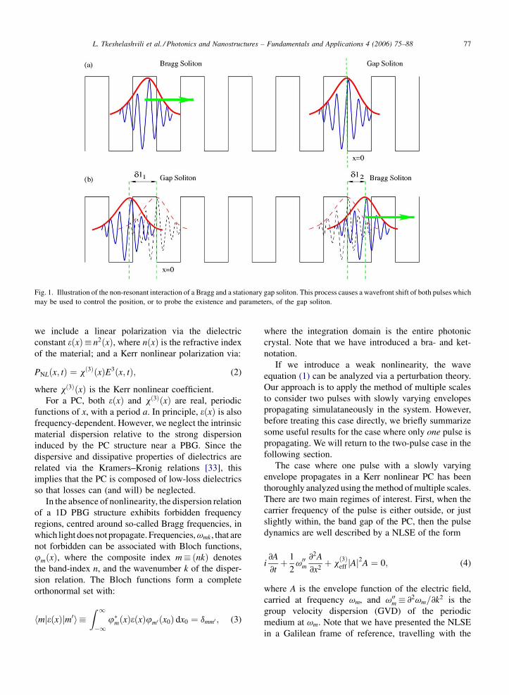
Fig. 1. Illustration of the non-resonant interaction of a Bragg and a stationary gap soliton. This process causes a wavefront shift of both pulses which
may be used to control the position, or to probe the existence and parameters, of the gap soliton.
we include a linear polarization via the dielectric
constant eðxÞ� n2ðxÞ, where nðxÞ is the refractive index
of the material; and a Kerr nonlinear polarization via:
PNLðx; tÞ ¼ xð3ÞðxÞE3ðx; tÞ; (2)
where xð3ÞðxÞ is the Kerr nonlinear coefficient.
For a PC, both eðxÞ and xð3ÞðxÞ are real, periodic
functions of x, with a period a. In principle, eðxÞ is also
frequency-dependent. However, we neglect the intrinsic
material dispersion relative to the strong dispersion
induced by the PC structure near a PBG. Since the
dispersive and dissipative properties of dielectrics are
related via the Kramers–Kronig relations [33], this
implies that the PC is composed of low-loss dielectrics
so that losses can (and will) be neglected.
In the absence of nonlinearity, the dispersion relation
of a 1D PBG structure exhibits forbidden frequency
regions, centred around so-called Bragg frequencies, in
which light does not propagate. Frequencies, vmk, that are
not forbidden can be associated with Bloch functions,
jmðxÞ, where the composite index m�ðnkÞ denotes
the band-index n, and the wavenumber k of the disper-
sion relation. The Bloch functions form a complete
orthonormal set with:
hmjeðxÞjm0i �Z 1�1
j�mðxÞeðxÞjm0 ðx0Þ dx0 ¼ dmm0 ; (3)
where the integration domain is the entire photonic
crystal. Note that we have introduced a bra- and ket-
notation.
If we introduce a weak nonlinearity, the wave
equation (1) can be analyzed via a perturbation theory.
Our approach is to apply the method of multiple scales
to consider two pulses with slowly varying envelopes
propagating simulataneously in the system. However,
before treating this case directly, we briefly summarize
some useful results for the case where only one pulse is
propagating. We will return to the two-pulse case in the
following section.
The case where one pulse with a slowly varying
envelope propagates in a Kerr nonlinear PC has been
thoroughly analyzed using the method of multiple scales.
There are two main regimes of interest. First, when the
carrier frequency of the pulse is either outside, or just
slightly within, the band gap of the PC, then the pulse
dynamics are well described by a NLSE of the form
i@A
@tþ 1
2v00m
@2A
@x2þ x
ð3Þeff jAj
2A ¼ 0; (4)
where A is the envelope function of the electric field,
carried at frequency vm, and v00m� @2vm=@k2 is the
group velocity dispersion (GVD) of the periodic
medium at vm. Note that we have presented the NLSE
in a Galilean frame of reference, travelling with the
L. Tkeshelashvili et al. / Photonics and Nanostructures – Fundamentals and Applications 4 (2006) 75–8878
group velocity (v0m) of the pulse. The effective nonlinear
coefficient in (4) is:
xð3Þeff ¼ 6pvm
Zxð3ÞðxÞjjmðxÞj
4dx: (5)
This overlap integral reflects the fact that the Bloch
functions are not uniformly distributed over the con-
stituent materials of a PC.
The NLSE (4) exhibits soliton solutions with a
familiar sech amplitude profile when the Lighthill
condition, xð3Þeff v
00m > 0, holds [34]. In Fig. 2 we show a
typical dispersion relation for a 1D PC in the vicinity
of a band gap. For frequencies above (below) the gap,
v00m is positive (negative). Therefore, for focusing
(defocusing) nonlinearities, where xð3Þeff > 0 (x
ð3Þeff < 0),
solitons can be formed only if the pulse carrier
frequency is near the upper (lower) band edge.
The NLSE can describe pulses with a carrier
frequency within the band gap. In this case the solition
solution is called a ‘gap soliton’. If the carrier frequency
of the pulse is outside the gap, the soliton is referred to
as a ‘Bragg soliton’. These two solution regimes are
indicated in Fig. 2. It is well known that gap solitons can
exhibit a vanishing propagation velocity [19,28].
Clearly, when the group velocity, vg, vanishes, no
energy is transported and the carrier wave of the pulse is
a standing wave, i.e., a Bloch function at the band edge.
Nonlinear pulses with zero group velocity correspond to
stationary solutions of Eq. (4) of the form:
Aðx; tÞ ¼ AstðxÞexp ð�idtÞ: (6)
The parameter d is the frequency detuning of the carrier
wave from the band edge into the gap [19].
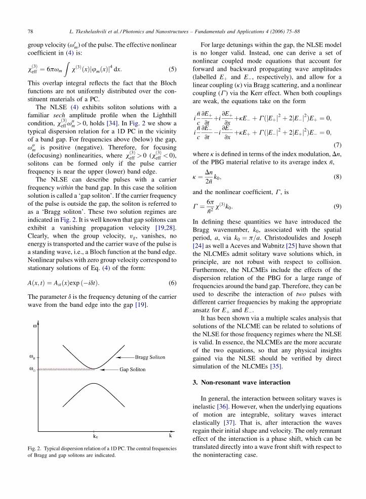
Fig. 2. Typical dispersion relation of a 1D PC. The central frequencies
of Bragg and gap solitons are indicated.
For large detunings within the gap, the NLSE model
is no longer valid. Instead, one can derive a set of
nonlinear coupled mode equations that account for
forward and backward propagating wave amplitudes
(labelled Eþ and E�, respectively), and allow for a
linear coupling (k) via Bragg scattering, and a nonlinear
coupling (G ) via the Kerr effect. When both couplings
are weak, the equations take on the form
in
c
@Eþ@tþi
@Eþ@xþkE� þ G ðjEþj2 þ 2jE�j2ÞEþ ¼ 0;
in
c
@E�@t�i
@E�@xþkEþ þ G ðjE�j2 þ 2jEþj2ÞE� ¼ 0;
(7)
where k is defined in terms of the index modulation, Dn,
of the PBG material relative to its average index n,
k ¼ Dn
2nk0; (8)
and the nonlinear coefficient, G , is
G ¼ 6p
n2xð3Þk0: (9)
In defining these quantities we have introduced the
Bragg wavenumber, k0, associated with the spatial
period, a, via k0 ¼ p=a. Christodoulides and Joseph
[24] as well a Aceves and Wabnitz [25] have shown that
the NLCMEs admit solitary wave solutions which, in
principle, are not robust with respect to collision.
Furthermore, the NLCMEs include the effects of the
dispersion relation of the PBG for a large range of
frequencies around the band gap. Therefore, they can be
used to describe the interaction of two pulses with
different carrier frequencies by making the appropriate
ansatz for Eþ and E�.
It has been shown via a multiple scales analysis that
solutions of the NLCME can be related to solutions of
the NLSE for those frequency regimes where the NLSE
is valid. In essence, the NLCMEs are the more accurate
of the two equations, so that any physical insights
gained via the NLSE should be verified by direct
simulation of the NLCMEs [35].
3. Non-resonant wave interaction
In general, the interaction between solitary waves is
inelastic [36]. However, when the underlying equations
of motion are integrable, solitary waves interact
elastically [37]. That is, after interaction the waves
regain their initial shape and velocity. The only remnant
effect of the interaction is a phase shift, which can be
translated directly into a wave front shift with respect to
the noninteracting case.

L. Tkeshelashvili et al. / Photonics and Nanostructures – Fundamentals and Applications 4 (2006) 75–88 79
Both elastic and inelastic collisions can be realized
within the NLSE model. Elastic collisions, generally
referred to as resonant interactions, take place when
the interacting solitons have very similar carrier
frequencies and, consequently, possess similar group
velocities and GVDs. This means that the interacting
pulses obey the NLSE with the same coefficients; and
the resonant interaction processes can be described
through the N-soliton solution of the NLSE [38,39].
Depending on the initial conditions, various resonant
effects such as soliton trapping and the formation of
bound states can be realized [36]. The spectral overlap
of the interacting solitons is essential for resonant
interaction. If this overlap is zero or negligible, the
solitons do not interfere coherently and resonant
interaction does not occur.
Inelastic collisions occur in the so-called non-
resonant regime [40,41]. In this regime, the interacting
solitons have sufficiently different group velocities that
they pass through each other quickly, thus avoiding
resonant effects. Note, in this regime, the interacting
solitons obey different NLSEs with different coeffi-
cients. In a PBG material, for example, a non-resonant
interaction could involve a stationary gap soliton and a
propagating Bragg soliton, as illustrated in Fig. 1. The
wave front shifts associated with non-resonant interac-
tions in PBG materials may have potential for
applications such as all-optical buffers, logic gates,
etc. [16]. In particular, as discussed in the introduction,
non-resonant interaction in PBG materials may be used:
(i) to launch stationary gap solitons by using Bragg
solitons to pull them into the PBG material; (ii) to probe
the existence and parameters of stationary gap solitons
through the corresponding shift of the colliding Bragg
soliton; and (iii) to control and manipulate the position
of a stationary gap soliton. However, we emphasize
these statements are valid only for the integrable NLSE
limit. When the equations of motion that govern the
nonlinear dynamics are non-integrable, inelastic effects
are present during the interaction processes. Below, we
will use inelastic interaction processes within the
NLCMEs synonymously with resonant processes.
Conversely, elastic processes within the NLCMEs
can be reduced to the NLSE model and may be resonant
or non-resonant. However, the non-resonant regime
remains associated with the NLSE regime only.
3.1. Multiple scales analysis of non-resonant
interaction
Here, we use the method of multiple scales to obtain
general analytical expressions for the nonlinear phase
shift induced by the non-resonant interaction of
solitons. We consider two pulses with different carrier
frequencies vmi (i ¼ 1; 2). These pulses may be in the
same band, n, at different wave vectors, k1 and k2, or in
different bands, n1 and n2, at the same or different wave
vectors.
As mentioned, the method of multiple scales has
been widely used to treat nonlinear problems in PBG
materials, and the reader is referred to those sources for
more details on the method. The basic idea is to
introduce a small parameter, m, that defines the
smallness of the nonlinear wave amplitude. We then
write the electric field, Eðx; tÞ, as [19]
Eðx; tÞ�m eðx; tÞ; (10)
where eðx; tÞ includes all perturbations which arise from
weak nonlinear processes:
eðx; tÞ ¼ e1ðx; tÞ þ m e2ðx; tÞ þ m2 e3ðx; tÞ þ � � � :(11)
Next, we formally replace the space and time variables,
x and t, with sets of independent spatial and temporal
variables fxn�mnxg and ftn�mntg, where n ¼0; 1; 2; . . . [22]. With this replacement, the functions,
ei, depend on all xn and all tn: eiðxÞ� eiðfxng; ftngÞ.However, for a perfectly periodic PC, the material
parameters are functions of the smallest length scale
x0 only, i.e. eðxÞ� eðx0Þ and xð3ÞðxÞ�xð3Þðx0Þ. For the
purposes of differentiation, the different spatial and
temporal variables are considered to be independent.
In our problem, we use the following ansatz for e1:
e1 ¼X2
i¼1
Aiðh1; h2; tÞjmiðx0Þexp ½�ivmi t0 þ imVmi �
þ c:c:; (12)
wherejm1ðx0Þ andjm2
ðx0Þ are the carrier waves (Bloch
functions) of the interacting pulses. Aiðh1; h2; tÞdenotes the slowly varying envelope function of the
ith wave, and Vmi ¼ Vmiðh1; h2; tÞ is the phase shift of
the ith wave after the interaction. The quantities, h1 and
h2, are related to the Galilean frame of reference
travelling with the respective pulses. In the absence
of the second pulse, h1 would be given by
h1 ¼ mðx� vg1tÞ, where vg1 is the group velocity of
pulse one at vm1. However, since the pulses interact, we
assume that Aiðh1; h2; tÞ and Vmiðh1; h2; tÞ depend on
the slow time variable,
t ¼ m2t: (13)

L. Tkeshelashvili et al. / Photonics and Nanostructures – Fundamentals and Applications 4 (2006) 75–8880
This means that the Galilean frames of the respective
pulses will also be slightly affected, at least during their
interaction. Consequently, we allow h1 and h2 to vary
during the interaction:
h1 ¼ mðx� vg1t � mcm1ðh1; h2; tÞÞ; (14)
h2 ¼ mðx� vg2t � mcm2ðh1; h2; tÞÞ: (15)
To generate a NLSE description, it is sufficient to
restrict the analysis to hi (i ¼ 1; 2) and t only. Clearly,
the carrier wave phase and wave front shifts, Vmi and
cmi, are not independent of each other. In the following,
we determine Vmi from the physical parameters of the
system, and subsequently determine cmi.
From Eqs. (13)–(15), the first order derivatives of an
arbitrary function Yðx0; t0; h1; h2; tÞ are
dY
dt¼ @Y
@t0
þ m
�� vg1
@Y
@h1
� vg2
@Y
@h2
�þ m2 @Y
@t; (16)
dY
dx¼ @Y
@x0
þ m
�@Y
@h1
þ @Y
@h2
�; (17)
and the second order derivatives are:
d2Y
dt2¼ @2Y
@t20
þ m2
�v2
g1
@2Y
@h21
þ 2vg1vg2
@2Y
@h1@h2
þ v2g2
@2Y
@h22
�;
(18)
d2Y
dx2¼ @2Y
@x20
þ m2
�@2Y
@h21
þ 2@2Y
@h1@h2
þ @2Y
@h22
�: (19)
Terms of order �m3 and higher are neglected in the
leading order of nonlinear effects considered here.
We now substitute Eqs. (10)–(12) into the wave
Eq. (1) and collect terms with the same power of m. This
determines the equations of motion for the correspond-
ing time and spatial scales.
3.1.1. The first order multi-scale analysis
In the lowest (first) order in m, we find:�� c2 @2
@x20
þ eðx0Þ@2
@t20
�e1 ¼ 0: (20)
Since this is just the wave equation for the PBG mate-
rial in the absence of nonlinearity, we find immedi-
ately that jm1ðx0Þ and jm2
ðx0Þ represent Bloch
functions with corresponding frequencies, vm1and
vm2, respectively.
3.1.2. The second order multi-scale analysis
To second order (terms of order m2), we find
�� c2 @2
@x20
þ eðx0Þ@2
@t20
�e2 ¼ Rð2Þ; (21)
where Rð2Þ is given by
Rð2Þ ¼�
2c2
�@A1
@h1
þ @A1
@h2
�@
@x0
jm1ðx0Þ
� 2ivm1eðx0Þ
�vg1
@A1
@h1
þ vg2
@A1
@h2
�jm1ðx0Þ
�exp ð�ivm1
t0Þ
þ�
2c2
�@A2
@h1
þ @A2
@h2
�@
@x0
jm2ðx0Þ
� 2ivm2eðx0Þ
�vg1
@A2
@h1
þ vg2
@A2
@h2
�jm2ðx0Þ
�exp ð�ivm2
t0Þ þ c:c:
(22)
We analyze Eqs. (21) and (22) using the following
Ansatz for e2
e2 ¼X1l1¼1
Bl1ðh1; h2; tÞjl1ðx0Þexp ð�ivm1
t0Þ
þX1l2¼1
Bl2ðh1; h2; tÞjl2ðx0Þexp ð�ivm2
t0Þ þ c:c:
(23)
Here the sum over l1 runs over all band indices at the
same (fixed) wave vector k1 associated with the carrier
wave m1�ðn1; k1Þ. Similarly, the sum over l2 extends
over all bands at the wave vector k2 associated with the
carrier wave m2�ðn2; k2Þ.Substituting (23) into Eqs. (21) and (22), we find
X1li¼1
ðv2li� v2
miÞeðx0Þjli
ðx0ÞBli
¼ 2i
�c
�@Ai
@h1
þ @Ai
@h2
�ð pjmi
ðx0ÞÞ
� vmieðx0Þ�
vg1
@Ai
@h1
þ vg2
@Ai
@h2
�jmiðx0Þ
�; (24)
where
p ¼ �ic@
@x0
: (25)

L. Tkeshelashvili et al. / Photonics and Nanostructures – Fundamentals and Applications 4 (2006) 75–88 81
Projecting Eq. (24) onto the carrier waves, jmiðx0Þ,
results in:
ðvg1 � vg2Þ@A1
@h2
¼ 0; (26)
ðvg1 � vg2Þ@A2
@h1
¼ 0; (27)
where we have made use of the orthonormality of the
Bloch functions (see Eq. (3)). Eqs. (26) and (27)
determine the quantitative condition for the realization
of the non-resonant interaction regime:
���� vg1 � vg2
vgi
�����m ði ¼ 1; 2Þ: (28)
When the group velocity of one of the interacting
waves, say, the first wave, is zero vg1 ¼ 0, Eq. (28)
must be replaced by nvg2=c�m, where n is the average
background index of refraction. These conditions
ensure that the interaction time of the two pulses is
sufficiently short that no resonant energy transfer can
take place.
We note that, according to Eqs. (26)–(28), in the non-
resonant interaction regime, the nonlinear wave
envelopes, A1 and A2, are decoupled, i.e.,
@A1
@h2
¼ @A2
@h1
¼ 0; (29)
so that Aiðh1; h2; tÞ�Aiðhi; tÞ. In addition, projecting
Eq. (24) onto all other Bloch functions jliðx0Þ at the
same wave vector as band mi (li 6¼mi), we obtain
expressions for the secondary envelope functions Bli ,
Bli �Bliðhi; tÞ ¼hlij pjmiiv2
li� v2
mi
@Ai
@hi
: (30)
Consequently, the secondary envelope functions, Bli ,
associated with the interacting waves are decoupled,
too. These secondary envelope functions ultimately
provide the group velocity dispersion for the primary
amplitudes, Ami (see [19]).
3.1.3. The third order multi-scale analysis
Finally, to third order in m, we find
�� c2 @2
@x20
þ eðx0Þ@2
@t20
�e3
¼ 4pv2m1
xð3Þðx0ÞRð3Þ1 þRð3Þ2 þR
ð3Þ3 ; (31)
where only Rð3Þ1 originates from the nonlinearity,
Rð3Þ1 ¼ ½3jjm1j2jm1
jA1j2A1
þ 6jjm2j2jm1
jA2j2A1�exp ð�ivm1t0Þ
þ ½3jjm2j2jm2
jA2j2A2
þ 6jjm1j2jm2
jA1j2A2�exp ð�ivm2t0Þ þ c:c:
(32)
In deriving Rð3Þ1 we have applied the rotating-wave
approximation.
The expressions for Rð3Þ2 and Rð3Þ3 are
Rð3Þ2 ¼X2
i¼1
2ivmi
X1li¼1
�c
vmi
ð pjliðx0ÞÞ � vgieðx0Þjli
ðx0Þ�
� @Bli
@hi
exp ð�ivmi t0Þ þ c:c:; (33)
and
Rð3Þ3 ¼X2
i¼1
�c2jmi
ðx0Þ@2
@h2i
Ai þ 2ic2
�@Vmi
@h1
þ @Vmi
@h2
�
� Ai@
@x0
jmiðx0Þ � eðx0Þjmi
ðx0Þ@2
@h2i
Ai
þ 2ivmieðx0Þjmiðx0Þ
@
@tAi
þ 2vmi
�vg1
@Vmi
@h1
þ vg2
@Vmi
@h2
�jmiðx0ÞAi
�
� exp ð�ivmi t0Þ þ c:c: (34)
The appropriate Ansatz for e3 is
e3 ¼X1l1¼1
Cl1ðh1; h2; tÞjl1ðx0Þexp ð�ivm1
t0Þ
þX1l2¼1
Cl2ðh1; h2; tÞjl2ðx0Þexp ð�ivm2
t0Þ þ c:c:;
(35)
where the sums obey the same rules as those in Eq.
(23).
Substituting Eq. (35) into Eq. (31) and projecting the
resulting expression onto jmiðx0Þ, we find that, as
expected, the envelope functions Ai of the interacting
pulses each obey the NLSE with corresponding
coefficients
i@Ai
@t2
þ 1
2v00mi
@2Ai
@h2i
þ xð3ÞeffijAij2Ai ¼ 0: (36)
More importantly, we find that the nonlinear phase
shift Vm1of the first wave depends only on the differ-
ence in group velocities, the effective cross phase

L. Tkeshelashvili et al. / Photonics and Nanostructures – Fundamentals and Applications 4 (2006) 75–8882
modulation Dð3Þeffi between the pulses and the amplitude
of the second wave
@
@h2
Vm1¼ D
ð3Þeff1
vg1 � vg2
jA2j2: (37)
The cross-phase modulation constant Deff1 is defined as
(cf. Eq. (5))
Dð3Þeff1 ¼ 12pvm1
Zxð3Þðx0Þjjm1
ðx0Þj2jjm2ðx0Þj2 dx0:
(38)
We note that, as a consequence of Eq. (37), Vm1
depends only on h2 and is independent of h1. The phase
shift of the second wave is given by a completely
analogous expression with the indices 1 and 2 inter-
changed.
Eq. (38) suggests that the interaction between
nonlinear pulses in the non-resonant regime is
determined by the overlap of the carrier Bloch functions
of the pulses. In particular, it is possible that the cross-
phase modulation between the pulses is enhanced, due
to the large overlap of the Bloch functions, jm1ðx0Þ and
jm2ðx0Þ, and the Kerr nonlinearity xð3Þðx0Þ. On the other
hand, when x3ðx0Þ changes sign within the unit cell, it
may happen that for certain pairs of frequencies the
overlap of the corresponding Bloch functions is zero. In
such situations non-resonant interaction effects would
be entirely absent.
3.2. The wave front shift
We now determine the wave front shift cmiasso-
ciated with the nonlinear phase shift Vmi . We consider
the group velocity of the first wave during the
interaction, which can be re-written as
dðvm1þ Dvm1
Þdðk1 þ Dk1Þ
¼�
1� dDk1
dk1
��dvm1
dk1
þ dDvm1
dk1
�ffi d
dk1
vm1
� d
dk1
Dk1
d
dk1
vm1þ d
dk1
Dvm1: (39)
Here, we have introduced the nonlinear wave vector
shift, Dk1, and the nonlinear frequency shift, Dvm1,
experienced by the first wave via interaction with the
second:
Dk1 ¼ m@
@xVm1¼ m2 @
@h2
Vm1(40)
Dvm1¼ �m
@
@tVm1¼ m2vg2
@
@h2
Vm1� vg2Dk1: (41)
In deriving these expressions, we used Eqs. (16) and
(17).
Thus, the nonlinear group velocity shift Dvg1 of the
first pulse during the interaction process becomes
Dvg1�dðvm1
þ Dvm1Þ
dðk1 þ Dk1Þ� d
dk1
vm1
¼ d
dk1
�Dvm1
��
d
dk1
vm1
�Dk1
�
¼ �m2ðvg1 � vg2Þd
dk1
�@
@h2
Vm1
�: (42)
These considerations suggest a clear physical inter-
pretation of the non-resonant wave interaction. The
local distortion of the photonic band structure induced
by one of the pulses appears to the other pulse as a
shift in the local group velocity. This is a reciprocal
effect and must be summed up over the duration of the
interaction process to produce the anticipated wave
fronts shifts of the interacting pulses relative to the
non-interacting case.
To carry out this summation, we derive from Eq. (14)
that
dh1
dt
����h1¼const
¼ dx
dt
����h1¼const
� vg1 � m@
@tcm1¼ 0:
(43)
Thus, we find an alternative expression for the nonlinear
group velocity shift, Dvg1:
Dvg1 ¼dx
dt
����h1¼const
� vg1 ¼ m@
@tcm1
; (44)
which directly implies the relation
Dvg1 ¼ mdh2
dt
����h1¼const
@
@h2
cm1
¼ m2ðvg1 � vg2Þ@
@h2
cm1: (45)
Based on Eqs. (42) and (45), we may now identify
@
@h2
cm1¼ � @
@k1
�@
@h2
Vm1
�: (46)
Eqs. (37), (38), and (46) give a complete description
of non-resonant interaction in the system. For insta-
nce, from Eq. (46) we can calculate the total wave front
shift, Dl1, of the first wave envelope A1:

L. Tkeshelashvili et al. / Photonics and Nanostructures – Fundamentals and Applications 4 (2006) 75–88 83
Dl1 ¼Z þ1�1
@
@h2
cm1dh2
¼ @
@k1
�Dð3Þeff1
ðvg2 � vg1Þ
� Z þ1�1jA2j2dh2: (47)
The second wave envelope, A2, experiences an
analogous shift, with indices changing from 1 to 2
and vice-versa. The implications of Eq. (47) are:
(i) we can control and modify the position of a non-
linear pulse (pulse one) by controlling the duration
and intensity of a collision partner (pulse two) and
(ii) the collision partner (pulse two) acquires a wave
front shift that provides information about the para-
meters of pulse one. Note, Eq. (47) is valid for pulses
well-described by the NLSE, i.e., for collisions of
Bragg solitons with Bragg or gap soliton as well as
for the collision of gap solitons with gap solitons. In
addition, Eq. (47) also describes the interaction of
extended waves with localized pulses. However, in
what follows we concentrate on collisions between
Bragg solitons and stationary gap solitons.
3.3. An example: fiber Bragg gratings
We now apply the formulae derived in the previous
section to a system with the physical parameters of a
fiber Bragg grating, which consists of a periodic
modulation of the index of refraction along the core of
an optical fiber [42]. The refractive index modulation is
usually weak (Dn=n 10�3) and the nonlinear pro-
cesses are well described by the nonlinear coupled
mode equations [28,26].
We consider the wave front shift, Dl1, of a stationary
(vg1� 0) gap soliton induced by a collision with a
propagating Bragg soliton (vg2 6¼ 0). We first note that
[28] for a 1D PC, the properly normalized (see Eq. 3)
Bloch functions in the upper band of the dispersion
relation can be written as:
jmiðx0Þ ¼
exp ðik x0Þffiffiffiffiffiffiffiffi2anp ½
ffiffiffiffiffiffiffiffiffiffiffiffiffiffi1þ vgi
p
�ffiffiffiffiffiffiffiffiffiffiffiffiffiffi1� vgi
pexp ð�2ik0 x0Þ�: (48)
The scaled group velocity, vgi ¼ nvgi=c, is defined with
respect to the group velocity for frequencies well away
from a Bragg resonance. Furthermore, we assume that
the nonlinear Kerr coefficient is constant along the fiber
(xð3Þðx0Þ ¼ xð3Þ0 ). We then find that the cross phase
modulation constant (38) is:
Dð3Þeff1 ¼
12pvm1xð3Þ0
an2
�1þ 1
2
ffiffiffiffiffiffiffiffiffiffiffiffiffiffiffiffiffiffiffiffiffiffiffiffiffiffiffiffiffiffiffiffiffiffiffiffið1� v2
g1Þð1� v2g2Þ
q �:
(49)
The intensity profile of the moving Bragg soliton
with the characteristic width, L2, is given by (see, for
instance, [38]):
jA2j2 ¼v00m2
xð3Þeff2L
22
1
cosh 2ðh2=L2Þ: (50)
And using (5) and (48), the effective nonlinearity (50)
is:
xð3Þeff2 ¼
3pvm2
an2xð3Þ0 ð3� v2
g2Þ: (51)
Substituting Eqs. (49)–(51) into Eq. (47) we arrive at the
wave front shift, Dl1, of the stationary gap soliton shift
after the collision:
Dl1 ¼8
k2L2
ð1� v2g2Þ
2
v2g2ð3� v2
g2Þ
�1þ 1
2
ffiffiffiffiffiffiffiffiffiffiffiffiffiffiffi1� v2
g2
q �: (52)
Analogously, the shift of the Bragg soliton, Dl2, is
Dl2 ¼8
3k2L1
�1� 2v2
g2
v2g2
�1þ 1
2
ffiffiffiffiffiffiffiffiffiffiffiffiffiffiffi1� v2
g2
q �
þ 1
2
ffiffiffiffiffiffiffiffiffiffiffiffiffiffiffi1� v2
g2
q �: (53)
In deriving (53) we have used the analytical expression
in [28] for the dispersion relation to calculate the GVD
of the two pulses.
From Eq. (52) it is apparent that to obtain a large
displacement of the stationary gap soliton, the values of
L2 and vg2 should be as small as possible. This is
expected, because the smaller the value of L2, the larger
the intensity of the moving soliton; similarly, for
smaller values of vg2, solitons interact for a longer time.
The soliton shifts are inversely proportional to the
square of the grating strength, k, because for smaller
values of k, the group velocity dispersion at the band
edge is larger [28], and consequently, the interacting
solitons have more energy. Finally, once the grating
strength, k, and the scaled velocity, vg2, of the Bragg
soliton are known, the Bragg soliton shift, Dl2, allows a
direct determination of the width, L1, of the stationary
gap soliton.
In the following section, we subject Eqs. (52) and
(53) to a detailed comparison with direct numerical
simulations of the NLCMEs (see also [29]).
L. Tkeshelashvili et al. / Photonics and Nanostructures – Fundamentals and Applications 4 (2006) 75–8884
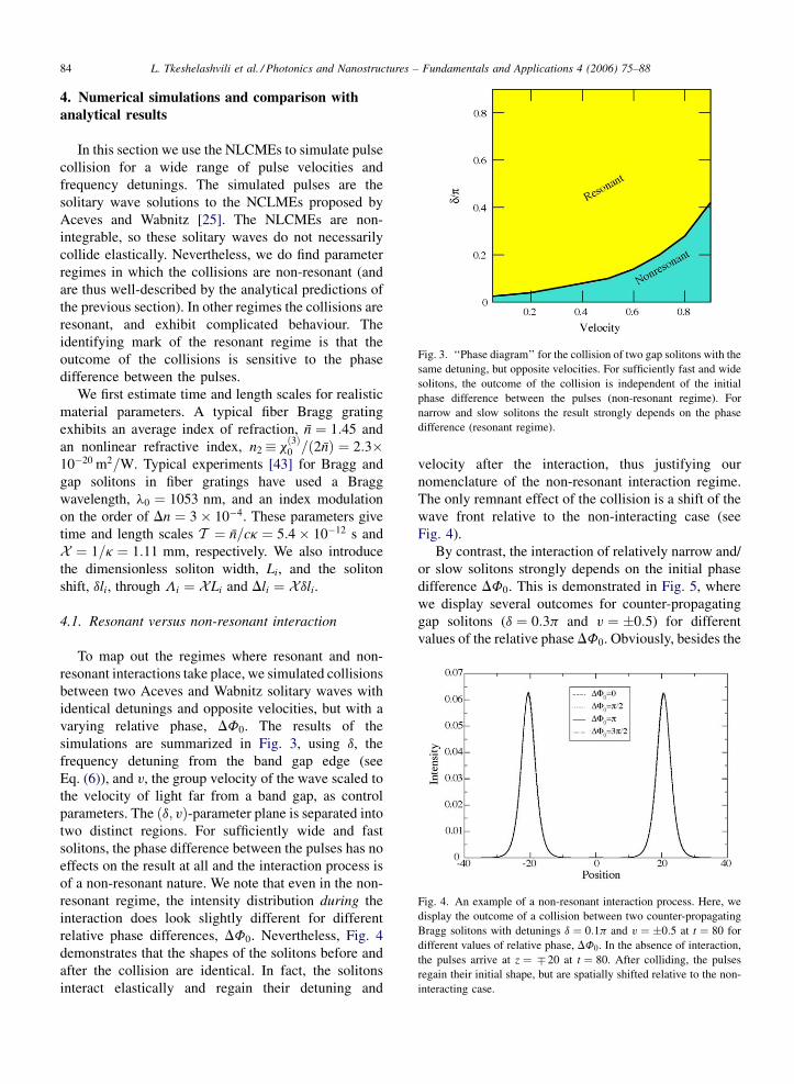
Fig. 3. ‘‘Phase diagram’’ for the collision of two gap solitons with the
same detuning, but opposite velocities. For sufficiently fast and wide
solitons, the outcome of the collision is independent of the initial
phase difference between the pulses (non-resonant regime). For
narrow and slow solitons the result strongly depends on the phase
difference (resonant regime).
Fig. 4. An example of a non-resonant interaction process. Here, we
display the outcome of a collision between two counter-propagating
Bragg solitons with detunings d ¼ 0:1p and v ¼ �0:5 at t ¼ 80 for
different values of relative phase, DF0. In the absence of interaction,
the pulses arrive at z ¼ � 20 at t ¼ 80. After colliding, the pulses
regain their initial shape, but are spatially shifted relative to the non-
interacting case.
4. Numerical simulations and comparison with
analytical results
In this section we use the NLCMEs to simulate pulse
collision for a wide range of pulse velocities and
frequency detunings. The simulated pulses are the
solitary wave solutions to the NCLMEs proposed by
Aceves and Wabnitz [25]. The NLCMEs are non-
integrable, so these solitary waves do not necessarily
collide elastically. Nevertheless, we do find parameter
regimes in which the collisions are non-resonant (and
are thus well-described by the analytical predictions of
the previous section). In other regimes the collisions are
resonant, and exhibit complicated behaviour. The
identifying mark of the resonant regime is that the
outcome of the collisions is sensitive to the phase
difference between the pulses.
We first estimate time and length scales for realistic
material parameters. A typical fiber Bragg grating
exhibits an average index of refraction, n ¼ 1:45 and
an nonlinear refractive index, n2�xð3Þ0 =ð2nÞ ¼ 2:3�
10�20 m2=W. Typical experiments [43] for Bragg and
gap solitons in fiber gratings have used a Bragg
wavelength, l0 ¼ 1053 nm, and an index modulation
on the order of Dn ¼ 3� 10�4. These parameters give
time and length scales T ¼ n=ck ¼ 5:4� 10�12 s and
X ¼ 1=k ¼ 1:11 mm, respectively. We also introduce
the dimensionless soliton width, Li, and the soliton
shift, dli, through Li ¼ XLi and Dli ¼ Xdli.
4.1. Resonant versus non-resonant interaction
To map out the regimes where resonant and non-
resonant interactions take place, we simulated collisions
between two Aceves and Wabnitz solitary waves with
identical detunings and opposite velocities, but with a
varying relative phase, DF0. The results of the
simulations are summarized in Fig. 3, using d, the
frequency detuning from the band gap edge (see
Eq. (6)), and v, the group velocity of the wave scaled to
the velocity of light far from a band gap, as control
parameters. The ðd; vÞ-parameter plane is separated into
two distinct regions. For sufficiently wide and fast
solitons, the phase difference between the pulses has no
effects on the result at all and the interaction process is
of a non-resonant nature. We note that even in the non-
resonant regime, the intensity distribution during the
interaction does look slightly different for different
relative phase differences, DF0. Nevertheless, Fig. 4
demonstrates that the shapes of the solitons before and
after the collision are identical. In fact, the solitons
interact elastically and regain their detuning and
velocity after the interaction, thus justifying our
nomenclature of the non-resonant interaction regime.
The only remnant effect of the collision is a shift of the
wave front relative to the non-interacting case (see
Fig. 4).
By contrast, the interaction of relatively narrow and/
or slow solitons strongly depends on the initial phase
difference DF0. This is demonstrated in Fig. 5, where
we display several outcomes for counter-propagating
gap solitons (d ¼ 0:3p and v ¼ �0:5) for different
values of the relative phase DF0. Obviously, besides the

L. Tkeshelashvili et al. / Photonics and Nanostructures – Fundamentals and Applications 4 (2006) 75–88 85
Fig. 5. Examples of resonant interaction processes. We show the
outcome of a collision between two gap solitons with d ¼ 0:3p and
v ¼ �0:5 at t ¼ 80 for different values of relative phase, DF0. In
contrast to the non-resonant case (Fig. 4), the shapes of the pulses after
interaction vary dramatically with DF0. Also, the velocities of the
emerging solitons strongly deviate from the launching velocity so that
at t ¼ 80, the positions of the pulses vary.
soliton position, the shapes of the pulses after
interaction are significantly different for different
relative phases, DF0. The nonlinear wave interaction
in this case is clearly resonant. In general, we find that
out-of-phase solitons (DF0 ¼ p) interact repulsively.
The centers of the solitons never ‘‘touch’’ and as long as
the solitons are wide and exhibit a sufficiently small
detuning, the interaction remains elastic. If the detuning
is too large, the solitons shed radiation and the collision
ceases to be elastic. The actual value of the velocity is
only of secondary interest in these cases. In some
extreme cases the solitons are completely destroyed. In
Fig. 6. (a) ‘‘Phase diagram’’ for the repulsive interaction of out-of-phase (D
sufficiently high detuning. (b) ‘‘Phase diagram’’ for the attractive interaction
identified. Soliton fusion occurs in the parameter region marked by ‘‘F’’ whi
dashed lines indicate ‘‘continuous’’ (or soft) transitions, between paramete
Fig. 6a, we display the boundary between elastic and
inelastic regime for the repulsive case.
For solitons that are in-phase (DF0 ¼ 0), the
interaction dynamics exhibits a much more compli-
cated behavior. In general, in-phase solitons interact
attractively, which means that during the interaction
all the energy is concentrated into a single sharp
intensity peak. The outcome of the collision depends
strongly on both the detuning and (somewhat less
strong) on the velocity. In the corresponding ‘‘phase
diagram’’ Fig. 6b, we can identify at least four different
interaction regimes.
For low values of the detuning, we are in the NLSE
limit where collisions are elastic. But within a region
of the detuning parameter between 0:18p and 0:3p and
for velocities below v ¼ 0:2, fusion of the colliding
solitons into one stationary pulse takes place. The
transition from the elastic scattering regime to the
fusion regime is rather abrupt. Very close to the border
between these regimes, we observe processes where
the solitons interact multiple times before finally
separating. These processes are accompanied by a
conspicuous spontaneous symmetry breaking, which
means the resulting solitons are no longer symmetric
with respect to the systems’ center of mass. Most
probably the reason for this is numerical noise, which
triggers an instability of the high-intensity peaks that
form during the interaction process. This instability
eventually leads to a breaking of symmetry. In [30],
Mak et al. suggest utilizing soliton fusion for creating
stationary light pulses. However, our detailed numer-
ical calculations indicate that in order to realize this
F0 ¼ p) pulses. The interaction changes from elastic to inelastic for
of in-phase DF0 ¼ 0 solitons. At least four parameter regimes can be
ch is separated from other region by abrupt boundaries. In contrast, the
rs regions of elastic, quasi-elastic, and strongly inelastic processes.

L. Tkeshelashvili et al. / Photonics and Nanostructures – Fundamentals and Applications 4 (2006) 75–8886
soliton fusion, the relative phase difference DF0 ¼ 0
between the pulses needs to be controlled with a
relative precision of better than 10�4. Otherwise, the
fusion to a stationary soliton does not take place and the
interacting pulses eventually separate from each other
after a highly complex interaction process. Therefore,
the experimental realization of the soliton fusion
process may prove to be challenging. As alluded to
above, for small detunings we find a regime of elastic
interactions where the NLSE is valid. However, for
intermediate detunings, the solitons interact quasi-
elastically, meaning their final velocity and energy
after the collision change relative to their launching
values, but their radiation losses are small (typically
below 1% of the total energy). Very close to the borders
with the fusion region, the solitons slow down after
colliding with each other. Everywhere else within the
quasi-elastic regime, the final velocities are higher
than the initial velocities. This difference in velocities
decreases with increasing initial velocities. Finally, for
large detunings, we enter an interaction regime where
the amount of radiation losses becomes so large that
during the interaction the solitons are completely
destroyed. We refer to this strongly inelastic regime as
the region of strong deformation. Except for the
transition to the fusion regime, transitions between any
of the regimes are ‘‘continuous’’ and in both the quasi-
elastic and the strong deformation region all processes
lead to radiation losses.
4.2. Giant soliton shifts
As alluded to in the previous sections, in the non-
resonant limit the collision between solitons is elastic
and their relative phase difference is of no consequence.
The only remnant effects of such interaction processes
Fig. 7. Wave front shifts of the stationary gap soliton (left panel) of fixed wid
Bragg soliton width L2. The dashed lines show the numerical results of the N
model (see Eqs. (52) and (53)).
are phase shifts associated with the soliton carrier
waves. Since the phase shift of a wave can be directly
translated into a corresponding wave front shift, after
the interaction process the center of each soliton will be
shifted relative to the noninteracting case. We have
given the analytical description of these processes
within the NLSE model in the previous section (see also
[29]). Here, we compare the analytical results of
Eqs. (52) and (53) via numerical simulations of colli-
sions between a stationary gap and moving Bragg
solitons using the NLCMEs. The results of these
simulations for widths L1 ¼ 5; and 40 of the stationary
gap soliton and widths L2 ¼ 5; 10; 20; and 40 of the
Bragg soliton are displayed in Figs. 7 and 8. We note
that fixing the width of the soliton uniquely determines
all soliton parameters for any given velocity [35]. In all
the cases described above, the corresponding detunings
are well below 0:15p, which means that the NLSE is
valid. The shifts, dl1, of the stationary gap soliton are
plotted in the left sub-figures; whereas, the correspond-
ing shifts, dl2, of the Bragg soliton are presented in the
right sub-figures. In each case, we fix the width, L1, of
the stationary gap soliton and vary the width, L2, of the
Bragg moving soliton. For comparison, we also plot the
analytic predictions (given by solid lines) based on
Eqs. (52) and (53). From Eqs. (52) and (53), it is
obvious that the analytic expression for the shift of one
soliton depends uniquely on the width of its collision
partner. As a result, we have that because the width of
the stationary gap soliton is fixed for each case, in
Figs. 7 and 8, the analytic predictions on the left panels
are always different; whereas, there is only one
analytical curve on the corresponding right panels.
Figs. 7 and 8 suggest that the wider the solitons, the
better agreement between the NLCMEs and the NLSE
predictions. This is expected, since it is precisely within
th L1 ¼ 5, and the Bragg soliton (right panel) for different values of the
LCMEs and the solid lines show the analytic predictions of the NLSE

L. Tkeshelashvili et al. / Photonics and Nanostructures – Fundamentals and Applications 4 (2006) 75–88 87
Fig. 9. Examples of collisions between gap and Bragg solitons. In the left panel, two solitons (L1 ¼ L2 ¼ 5 and v2 ¼ 0:05) collide non-resonantly,
and both pulses experience a giant wavefront shift relative to the non-interacting case. The right panel depicts a quasi-elastic interaction process
between the solitons (L1 ¼ L2 ¼ 2:5 and v2 ¼ 0:05), in which the initially stationary gap soliton becomes mobile after the collision.
Fig. 8. Wave front shifts of the stationary gap soliton (left panel) of fixed width L1 ¼ 40, and the Bragg soliton (right panel) for different values of the
Bragg soliton width L2. The dashed lines show the numerical results of the NLCMEs and the solid lines show the analytic predictions of the NLSE
model (see Eqs. (52) and (53)).
this limit that the NLCMEs reduce to the NLSE. If both
solitons are very narrow, then both wave front shifts
start to oscillate as a function of the Bragg soliton’s
velocity. This behavior signals that resonant effects are
starting to become increasingly important and/or the
collisions are no longer elastic. A typical example of
non-resonant collisions between gap and Bragg solitons
that lead to giant wave front shifts is depicted in the left
panel of Fig. 9. A typical inelastic interaction process,
as displayed in the right panel of Fig. 9, allows the
initially stationary solitons to become mobile after the
collisions, which makes it very difficult to accurately
define and measure the wave front shifts.
For the typical experimental values given above, the
soliton shifts are of the order of millimeters or even
centimeters. This is several orders of magnitude larger
than the corresponding shifts found in ordinary fibers
(without a grating). This observation makes nonlinear
PBG materials particularly interesting for certain
applications of these effects.
5. Conclusions
In conclusion, we have studied, both analytically and
numerically, nonlinear wave interaction processes in
one-dimensional photonic band gap materials.
The non-resonant interaction of nonlinear pulses
may lead to efficient mechanisms for dynamically
controlling optical waves. In particular, for realistic
systems the analytical formulae predict that the wave
front shift experienced by these pulses is of the order of
millimeters or even centimeters. Such pronounced
effects should be easily observable in the laboratory.
Moreover, the non-resonant interaction processes can
be utilized to control the position of stationary gap
solitons and to probe their very existence as well as their
physical parameters. Furthermore, the direction of this
research suggests that non-resonant interaction might
be useful for launching stationary gap solitons.
Numerical simulations confirm the analytical pre-
dictions for the regime of non-resonant interactions.

L. Tkeshelashvili et al. / Photonics and Nanostructures – Fundamentals and Applications 4 (2006) 75–8888
In addition, these simulations have allowed us to investi-
gate the inelastic wave interaction regime, for which
analytical results are unavailable. Our comprehensive
numerical studies demonstrate that, quite generally,
nonlinear wave interaction processes are very sensitive to
the relative phase of colliding pulses.
Finally, we would like to note that both the NLCMEs
and, in particular, the NLSE govern the nonlinear
dynamics of a large variety of physical systems,
including nonlinear optical and magnetic systems,
Bose–Einstein condensates, etc. This suggests that the
results presented in this paper are directly applicable to
other periodic structures of current interest. Most
notably, Bragg and gap solitons have been discussed
[44,45] and very recently observed [46] in Bose–
Einstein condensates in optical lattices.
Acknowledgements
L.T., J.N. and K.B. acknowledge the support by the
Center for Functional Nanostructures (CFN) of the
Deutsche Forschungsgemeinschaft (DFG) at the Uni-
versitat Karlsruhe within project A1.2. S.P. acknowl-
edges the support of the Natural Sciences and
Engineering Research Council of Canada (NSERC).
References
[1] J.D. Joannopoulos, P.R. Villeneuve, S. Fan, Nature 386 (1997)
143.
[2] S. John, O. Toader, K. Busch, Encyclopedia of Physical Science
and Technology, vol. 12, Academic Press, 2001.
[3] E. Yablonovitch, Phys. Rev. Lett. 58 (1987) 2059.
[4] S. John, Phys. Rev. Lett. 58 (1987) 2486.
[5] S. John, J. Wang, Phys. Rev. Lett. 64 (1990) 2418.
[6] P.St.J. Russell, Phys. Rev. A 33 (1986) 3232.
[7] H. Kosaka, et al. Phys. Rev. B 58 (1999) R10096.
[8] M. Scalora, et al. Phys. Rev. Lett. 73 (1994) 1368.
[9] H.G. Winful, J.H. Marburger, E. Garmire, Appl. Phys. Lett. 35
(1979) 379.
[10] N.D. Sankey, D.F. Prelewsitz, T.G. Brown, Appl. Phys. Lett. 60
(1992) 1427.
[11] C.J. Herbert, M.S. Malcuit, Opt. Lett. 18 (1993) 1783.
[12] W. Chen, D.L. Mills, Phys. Rev. Lett. 58 (1987) 160.
[13] D.L. Mills, S.E. Trullinger, Phys. Rev. B 36 (1987) 947.
[14] S. John, N. Akozbek, Phys. Rev. Lett. 71 (1993) 1168.
[15] S. John, N. Akozbek, Phys. Rev. E 57 (1998) 2287.
[16] A.B. Aceves, Chaos 10 (2000) 584.
[17] A.A. Sukhorukov, Y.S. Kivshar, Phys. Rev. E 65 (2002) 2287.
[18] U. Mohideen, et al. Opt. Lett. 20 (1995) 1674.
[19] C.M. de Sterke, J.E. Sipe, Phys. Rev. A 38 (1988) 5149.
[20] C.M. de Sterke, J.E. Sipe, Phys. Rev. A 39 (1989) 5163.
[21] C.M. de Sterke, J.E. Sipe, Phys. Rev. A 42 (1990) 550.
[22] T. Taniuti, Progr. Theor. Phys. (Suppl.) 55 (1974) 1.
[23] H.G. Winful, Appl. Phys. Lett. 46 (1985) 527.
[24] D.N. Christodoulides, R.I. Joseph, Phys. Rev. Lett. 62 (1989)
1746.
[25] A.B. Aceves, S. Wabnitz, Phys. Lett. A 141 (1989) 37.
[26] B.J. Eggleton, et al. Phys. Rev. Lett. 76 (1996) 1627.
[27] K. Busch, G. Schneider, L. Tkeshelashvili, H. Uecker, Zeitschrift
fur Angewandte Mathematik und Physik (ZAMP), in press.
[28] C.M. de Sterke, J.E. Sipe, in: E. Wolf (Ed.), Progress in Optics,
vol. XXXIII, Elsevier Science, Amsterdam, 1994, p. 203.
[29] L. Tkeshelashvili, S. Pereira, K. Busch, Europhys. Lett. 68
(2004) 205.
[30] W.C.K. Mak, B.A. Malomed, P.L. Chu, Phys. Rev. E 68 (2003)
026609.
[31] J.D. Jackson, Classical Electrodynamics, John Wiley & Sons,
Inc., New York, 1999.
[32] M. Born, E. Wolf, Principles of Optics, Pergamon Press, Oxford,
1964.
[33] C.P. Slichter, Principles of Magnetic Resonance, Springer-
Verlag, Berlin, 1992.
[34] M.J. Lighthill, Proc. R. Soc. A 229 (1967) 28.
[35] R.H. Goodman, R.E. Slusher, M.I. Weinstein, J. Opt. Soc. Am. B
19 (2002) 1635.
[36] G.I. Stegeman, M. Segev, Science 286 (1999) 1518.
[37] M.J. Ablowitz, H. Segur, Solitons and the Inverse Scattering
Transform, SIAM, Philadelphia, 1981.
[38] V.E. Zakharov, A.B. Shabat, Sov. Phys. JETP 34 (1972) 62.
[39] J.P. Gordon, Opt. Lett. 8 (1983) 596.
[40] M. Oikawa, N. Yajima, J. Phys. Soc. Jpn. 37 (1974) 486.
[41] M. Oikawa, N. Yajima, Progr. Theor. Phys. (Suppl.) 55 (1974)
36.
[42] A. Othonos, K. Kalli, Fiber Bragg Gratings, Artech House, Inc.,
Boston, 1999.
[43] B.J. Eggleton, C.M. de Sterke, J. Opt. Soc. Am. B 14 (1997)
2980.
[44] O. Zobay, et al. Phys. Rev. A 59 (1999) 643.
[45] R.G. Scott, et al. Phys. Rev. Lett. 90 (2003) 110404.
[46] B. Eiermann, et al. Phys. Rev. Lett. 92 (2004) 230401.