the age of information in situation awareness …...the age of information in situation awareness...
TRANSCRIPT
The Age of Information in Situation
Awareness Networks
Master internship report MN-420699
Jori Selen* 0637922Supervisors Ivo Adan*, Lachlan Andrew�, Yoni Nazarathy��, Hai Le Vu �
September 22, 2012
*Manufacturing Networks Group, Department of Mechanical Engineering, Eind-hoven University of Technology, Eindhoven, Netherlands
�Centre for Advanced Internet Architectures, Faculty of Information and Com-munication Technologies, Swinburne University of Technology, Melbourne, Aus-tralia
�School of Probability and Statistics, The University of Queensland, Brisbane,Australia
Abstract
In this paper we derive analytical distributions up to a bounding box of theage of information in situation awareness networks. Two special cases ofthese networks are studied which leads to the derivation of two algorithms.We find that each node in a tree structured network has a generalized neg-ative binomial marginal distribution. Finally, we consider two branches ofnodes leading from source to a sink and design an algorithm (using the previ-ous algorithms) that is capable of obtaining joint and marginal distributionsof these nodes. The algorithm iteratively computes segments of the totaljoint distribution and therefore keeps time and memory usage manageable.
Contents
1 Introduction 3
2 A general model 5
2.1 Bernoulli channels 6
2.2 Bernoulli policies 7
2.3 Reception probabilities induced by Bernoulli channels andpolicies 8
2.4 Implication of the transceiver and interference principles ona homogeneous system 10
3 Single hop networks 12
3.1 One single hop 14
3.2 Two single hops 15
3.3 Three single hops 19
3.4 Arbitrary number of single hops 21
3.5 Minimum over a joint distribution of a single hop network 23
4 Line of relays 25
5 A network with two branches 30
5.1 The 3-dimensional case 32
5.2 The 4-dimensional case 35
5.3 Iterating over two branches 37
6 Conclusion 45
A Derivation of the covariance for a network with two singlehops 48
B M-file: Function for computing λj(B) 52
1
C M-file: Computing the 4-dimensional iterate 55
D M-file: Using the iteration scheme 60
2
Chapter 1
Introduction
In broadest generality, a situation awareness network or gossip network canbest be described as a network of nodes that can sense, transmit, relay andreceive information. The type of information can range from weather mea-surements to road traffic conditions to enemy military vehicles. In such anetwork, each node wants a most updated view of all the available informa-tion. Deriving a policy on whether to sense, transmit, relay or receive is oneof the main topics of study.
Situation awareness networks are becoming more prevalent in the researchfields and in practice. A large part of this field is the study of road trafficnetworks, where cars transmit, relay and receive information about con-gestion or blockage. Information propagation in these networks is studiedextensively. A measure of performance for such networks is the time un-til all nodes are fully aware of all information. These networks are usuallystudied through the use of simulation and deriving conjectures from thesesimulations that can later be proven.
This report focuses on an analytic approach of situation awareness networks.We consider static communicating nodes and are interested in the age ofinformation one node has about another node. A general, abstract modelis introduced where the type of information is undefined. The model canlater be specialized towards one type of network, this is beyond the scopeof this study. The main goal is to design an algorithm capable of iteratinga joint distribution of ages of information along two branches of nodes froma source to a sink. Using this algorithm, marginal and joint distributions ofages of information with respect to a chosen source can be studied.
In the literature we find that queuing networks with catastrophes, such as[2], are related to the age of information in situation awareness networks.A study on gossip networks in [1] focuses on propagation of information innetworks with mobile nodes. Another link can be made to PERT, a projectplanning analysis, which is a type of shortest (or critical) path problem.
3
Articles such as [3], [4] and [5] discuss PERT problems with dependentactivities and means of solving these. These different fields are all related toour general model and can be used, yet differ enough for this to be a uniquestudy.
We commence with an introduction of the general model in Chapter 2, themodel will be made more specific by introducing a policy on the receptionand transmission behaviour in one of the later sections. Chapters 3 and 4discuss two special cases of the general model, for both cases an algorithmis sought. The penultimate chapter, Chapter 5, discusses the design of analgorithm that can be used in iterating over two branches of nodes. Thereport is concluded in the final chapter.
4
Chapter 2
A general model
In this chapter we introduce the general model of the situation awarenessnetwork. More structure is given to this model throughout Sections 2.1and 2.2 by introducing assumptions and policies on transmission and recep-tion behaviour. The final sections investigate the effects of the proposedassumptions.
Consider a network of N nodes, N = {1, . . . , N}. Each node performssensing, wireless communication and uses the information sensed by theother nodes of the network. Each node attempts to maintain an updatedsituation awareness view of the information sensed by all other nodes inthe network, yet it may be that the information is not always up to date.Nodes communicate by broadcasting. When a node broadcasts, it sendsa packet that contains a subset of its situation awareness view. This maycontain the information sensed by the node, as well as information takenfrom its situation awareness view regarding other nodes at earlier times.Thus nodes essentially relay sensor information. Note that we assume thatif node i broadcast its situation awareness view about node j, it sent all ofthe information regarding that node as well as a time stamp of the age of thatinformation. Nodes can not receive information when they are broadcastingthemselves, analogous to a transceiver.
We assume the network evolves in discrete (slotted) time n = 0, 1, 2, . . ..The situation awareness age process is {Xn(i, j), n = 0, 1, . . . , (i, j) ∈ N 2}.This is essentially the state of our system. The element Xn(i, j) is the age ofthe information that node i has about node j at time n. Thus for exampleif Xn(1, 3) = 15, we know that at time n, node 1’s most updated viewregarding the sensed information at node 3 is from time n− 15.
Given initial conditions, X0(·), the evolution of Xn(·) is driven by the fol-lowing objects: the binary matrix sequence of information transmissions{In(i, j), n = 0, 1, . . . , (i, j) ∈ N 2}, the binary vector sequence of infor-mation sensing {Fn(i), n = 0, 1, . . . , i ∈ N} and the sequence of channel
5
functions {Cn, n = 0, 1, . . .} where Cn : {0, 1}N → {0, 1}N×N . For the infor-mation transmission sequence, we have that In(i, j) = 1 if and only if at timen node i has broadcasted its information regarding node j. For the sensingsequence, we have that Fn(i) = 1 if and only if at time n node i has updatedits own sensor information (by sensing). For the operation of the chan-nel functions, we use an additional variable, Tn(i) = 1{
∑Nj=1 In(i, j) ≥ 1},
where 1{} is the indicator function. This sequence determines if node ibroadcasted a packet at time n (note that all sensor information that ibroadcasts is assumed to sit on one packet). Now the function Cn(Tn) re-sults in the matrix with elements Rn(i, j) where Rn(i, j) = 1 if and onlyif j received a packet sent by node i. The diagonal elements Rn(i, i) aremeaningless and set to 0. Note that we restrict the sequence Cn to result inRn(i, j) = 1 only if Tn(i) = 1.
Given the above primitives, the evolution of the situation awareness age isas follows:
Xn+1(i, j) =
{ (Xn(i, j) ∧
∧k:Rn(k,i)In(k,j)=1Xn(k, j)
)+ 1 i 6= j,
(1− Fn(i))(Xn(i, i) + 1) i = j.
(2.1)
The symbol∧i is used to indicate taking a minimum over i. Observe that the
variables that drive the recursion are the initial conditions, X0, the broad-casts In, the sensing actions Fn and the channel conditions Cn. A minimumis taken over the set of information pieces regarding node j that have beenreceived by node i. Each node is only interested in the youngest informationand therefore compares the minimum age of information that was receivedwith the current age of information stored in node i. The channel plays arole here in transforming In first to Tn (putting information pieces in trans-mitted packets) and then through Cn (which models packet losses) to Rn.Further note that if we ignore the sensing actions by assuming that eachnode performs sensing at every time instant, we have that Xn(i, i) = 0.
The above model is very general and without probabilistic assumptions. Wenarrow down, but still remain fairly general. First we ignore the degree offreedom of sensing and assume Fn(i) ≡ 1, a node will always have perfectinformation about itself and therefore Xn(i, i) = 0 as stated earlier. In thenext sections Bernoulli channels and policies are introduced. These governthe transmission and reception behaviour.
2.1 Bernoulli channels
An approximation of real-life communication channels is made by introduc-ing a Bernoulli variable governing reception of a signal. We shall assumethe channel functions, Cn are an i.i.d. sequence with the following structure:
6
for all i, j ∈ N and A ⊂ N , let pij(A) indicate the probability of successfulreception at node j of packet transmitted at node i when the set of trans-mitting stations is A, where A = {k : Tn(k) = 1}. Require that pij(A) = 0if i 6∈ A. Now assume that the i, j’th entry of Cn(Tn) is a bernoulli randomvariable taking 1 with probability pij(A) and 0 otherwise, independent of allother random variables. The probability pij(A) is a function of the trans-mitting nodes to incorporate for interference and for the fact that we dealwith nodes that can not receive and transmit at the same time.
It is sensible to assume that if i ∈ A,B and A ⊂ B then pij(A) ≥ pij(B).Thus pij({i}) is the success probability on i→ j without any possible inter-ference from any other node. We denote this probability as pij for short.
We impose a graph structure between the nodes by specifying a set of di-rected links. We can then define the set of neighbours of node j as Kj . Thenodes in the set Kj are the nodes that can influence the reception proba-bility of node j, i.e. nodes that are close by or nodes that have a powerfulsignal, disrupting other communication over large distances. We can modelinterference of other broadcasting nodes by a decreasing interference func-tion L, depending on the transmitting nodes that affect the receiving node.Other broadcasting nodes, which are not neighbours, do not influence thereception probabilities. The proposed success probability is defined as
pij(A) = 1{j /∈ A}L(A ∩Kj)pij . (2.2)
Note that pij(A) = pij(A ∩Kj) which is desired behaviour, and we cannotreceive if we are transmitting. A choice can be made for the interferencefunction L, one can think of mutual exclusiveness, which can be described as,if some neighbouring node of node j is transmitting, node j cannot receive.Another option is a decreasing function over the number of transmittingneighbouring nodes, e.g. L = 1
|A∩Kj |+1 . One can also study the behaviour
when there is no interference by setting L to 1.
2.2 Bernoulli policies
The transmission control of the nodes in the network is governed by In(i, j).Recall that In(i, j) = 1 if and only if at time n node i has broadcasted itsinformation regarding node j. A policy on the transmission probabilities isan engineering decision, not a model of nature. One could opt for a differentpolicy that is not treated in the report. We shall now describe policieswhere In is an i.i.d. sequence, independent of the state and refer to these asBernoulli policies. In greatest generality we have a probability distributionfunction overN 2 indicating the probability of transmission of each subset. Away to define this is to assume that In(i, j) equals 1 with probability qij and0 otherwise, independent of all other i and j. This implies that each node
7
i transmits a random number of information updates, which can also be 0,because qi = 1−
∏j(1− qij) ≤ 1. An alternative way is to assume that each
node will transmit all bits of information with probability qi (independentlyof all other nodes). In this report we solely focus on the first option andlook at just one type of information being sent or relayed, i.e. j is a nodethat does not change, labeled as the source.
2.3 Reception probabilities induced by Bernoullichannels and policies
In the previous two sections the Bernoulli channels and policies were intro-duced. These channels and policies induce a successful reception probabil-ity. Let {γj(B) : B ⊂ N} be the one-step probability distribution indicatingfrom which sensors reception will occur at node j, where B is the set of nodesfrom which the successful reception occurs. We can write this in terms ofthe given parameters as
γj(B) =∑
D:B⊂D⊂N
∏i∈N\D
(1− qi)∏i∈D
qi∏i∈B
pij(D)∏
i∈D\B
(1− pij(D)). (2.3)
One can edit equation (2.3) by interchanging qi for qik for a specific nodek to obtain the probabilities of receiving a specific packet of information(about node k). This is useful in assessing the probabilities of updates onXn(j, k). Let us also define, for B ⊂ C ⊂ N
γj(B;C) =∑
D:D⊂N\C
γj(B ∪D).
This is the modified probability of reception γj , given that we only take thenodes in set C into account, i.e. we look at a subset of the whole networkand want to know the probabilities of reception.
Equation (2.3) can also be altered to obtain the probability of successfulreception of one specific type of information throughout the whole network.Let {λj(B) : B ⊂ N} be the one-step probability distribution over allsubsets of N indicating which sensor receives information about source j.Specifically, this can only be used in networks that have a tree-structure. Insuch networks, each node has only one possible incoming transmission butis allowed to transmit to multiple nodes.
λj(B) =∑
D:A⊂D⊂N
∏i∈N\D
(1− qij)∏i∈D
qij∏i∈B
pi(D)∏
i∈D\B
(1− pi(D)) (2.4)
Note that there is only a subtle difference between γj and λj . We haveintroduced the probability pi(A) which denotes the probability of reception
8
at node i given that nodes A are transmitting. It is defined analogous to(2.2), where Kj is now defined as the set of neighbours that could causeinterference at node j and pij is interchanged for pi. Recall that there isonly one possible incoming transmission at node i. The variable λj will beused to great extent in analyzing networks that have a tree-structure. Onceagain, let us also define, for B ⊂ C ⊂ N
λj(B;C) =∑
D:D⊂N\C
λj(B ∪D). (2.5)
Throughout the rest of this report, tree structures will be studied to greatextent and therefore the variable λj(B) is used in numerous cases. The M-file used to compute these probabilities of successful reception is shown inAppendix B.
9
2.4 Implication of the transceiver and interferenceprinciples on a homogeneous system
The general model introduced the principle of a transceiver, nodes cannotreceive information when they are transmitting information themselves. Onecould argue that there should be some optimal value for probability of trans-mission qi. If we set qi to either 0 or 1 for all i, there will not be reception onany of the nodes. We illustrate this optimal value by treating an example.
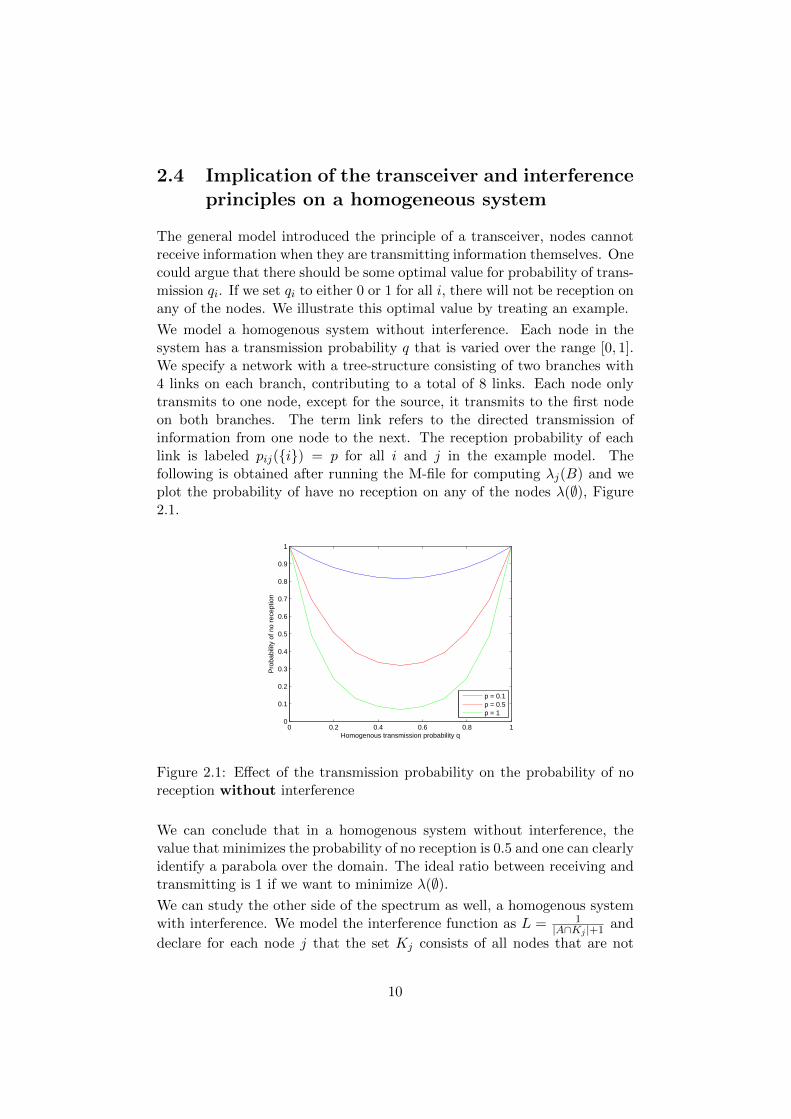
We model a homogenous system without interference. Each node in thesystem has a transmission probability q that is varied over the range [0, 1].We specify a network with a tree-structure consisting of two branches with4 links on each branch, contributing to a total of 8 links. Each node onlytransmits to one node, except for the source, it transmits to the first nodeon both branches. The term link refers to the directed transmission ofinformation from one node to the next. The reception probability of eachlink is labeled pij({i}) = p for all i and j in the example model. Thefollowing is obtained after running the M-file for computing λj(B) and weplot the probability of have no reception on any of the nodes λ(∅), Figure2.1.
0 0.2 0.4 0.6 0.8 10
0.1
0.2
0.3
0.4
0.5
0.6
0.7
0.8
0.9
1
Homogenous transmission probability q
Pro
babi
lity
of n
o re
cept
ion
p = 0.1p = 0.5p = 1
Figure 2.1: Effect of the transmission probability on the probability of noreception without interference
We can conclude that in a homogenous system without interference, thevalue that minimizes the probability of no reception is 0.5 and one can clearlyidentify a parabola over the domain. The ideal ratio between receiving andtransmitting is 1 if we want to minimize λ(∅).We can study the other side of the spectrum as well, a homogenous systemwith interference. We model the interference function as L = 1
|A∩Kj |+1 and
declare for each node j that the set Kj consists of all nodes that are not
10
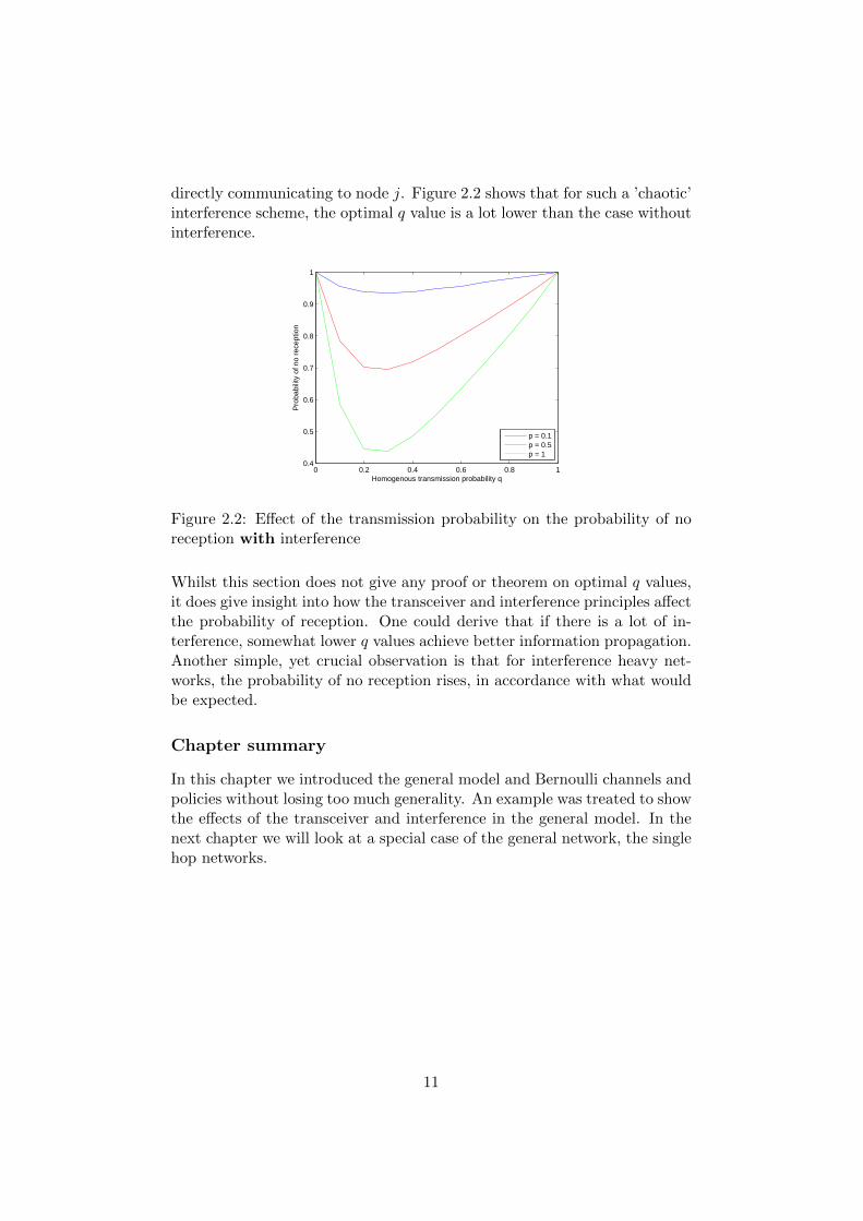
directly communicating to node j. Figure 2.2 shows that for such a ’chaotic’interference scheme, the optimal q value is a lot lower than the case withoutinterference.
0 0.2 0.4 0.6 0.8 10.4
0.5
0.6
0.7
0.8
0.9
1
Homogenous transmission probability q
Pro
babi
lity
of n
o re
cept
ion
p = 0.1p = 0.5p = 1
Figure 2.2: Effect of the transmission probability on the probability of noreception with interference
Whilst this section does not give any proof or theorem on optimal q values,it does give insight into how the transceiver and interference principles affectthe probability of reception. One could derive that if there is a lot of in-terference, somewhat lower q values achieve better information propagation.Another simple, yet crucial observation is that for interference heavy net-works, the probability of no reception rises, in accordance with what wouldbe expected.
Chapter summary
In this chapter we introduced the general model and Bernoulli channels andpolicies without losing too much generality. An example was treated to showthe effects of the transceiver and interference in the general model. In thenext chapter we will look at a special case of the general network, the singlehop networks.
11
Chapter 3
Single hop networks
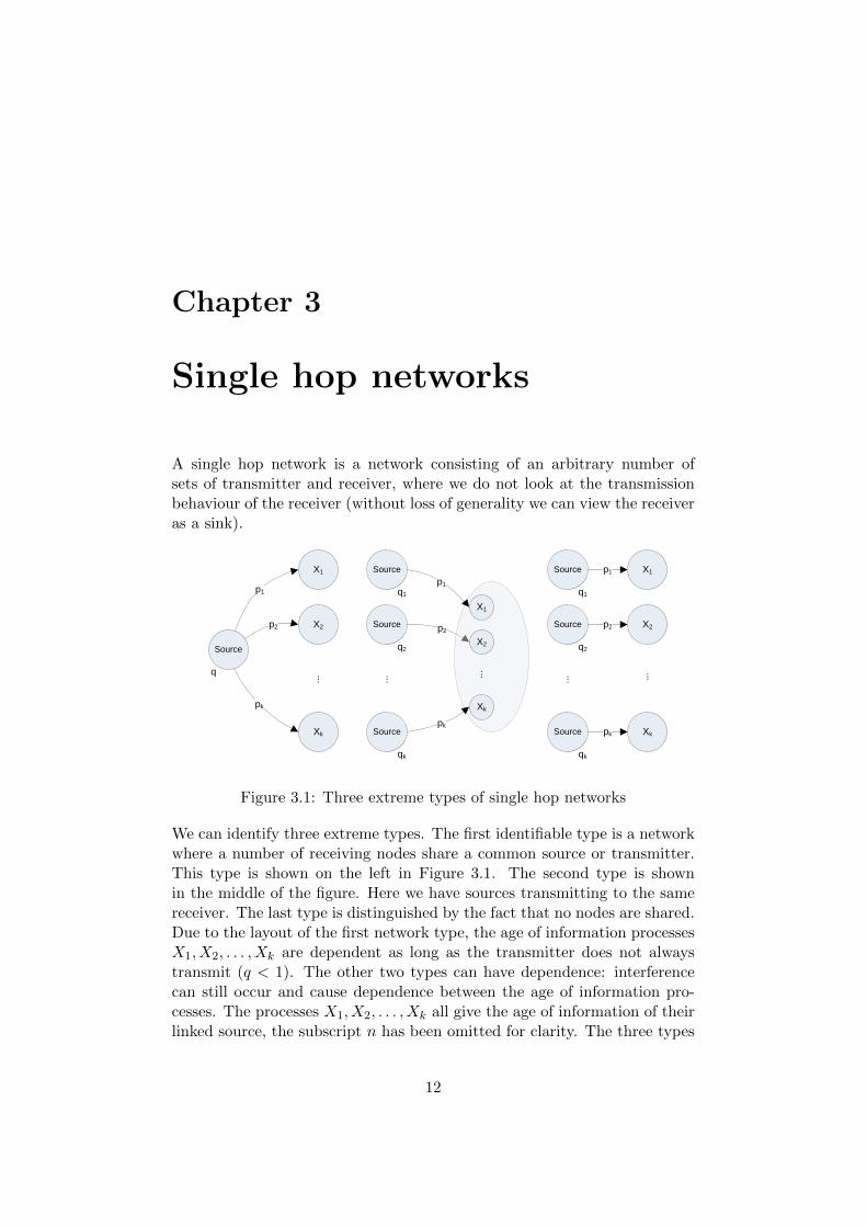
A single hop network is a network consisting of an arbitrary number ofsets of transmitter and receiver, where we do not look at the transmissionbehaviour of the receiver (without loss of generality we can view the receiveras a sink).
Source
X1
X2
Xk
p1
p2
...
pk
q
q1
qk
Source
Source
Source
X2
Xk
...
X1
...
p1
pk
q2
X1
X2
Xk
...
q1
qk
Source
Source
Source
q2
...
p1
p2
pk
p2
Figure 3.1: Three extreme types of single hop networks
We can identify three extreme types. The first identifiable type is a networkwhere a number of receiving nodes share a common source or transmitter.This type is shown on the left in Figure 3.1. The second type is shownin the middle of the figure. Here we have sources transmitting to the samereceiver. The last type is distinguished by the fact that no nodes are shared.Due to the layout of the first network type, the age of information processesX1, X2, . . . , Xk are dependent as long as the transmitter does not alwaystransmit (q < 1). The other two types can have dependence: interferencecan still occur and cause dependence between the age of information pro-cesses. The processes X1, X2, . . . , Xk all give the age of information of theirlinked source, the subscript n has been omitted for clarity. The three types
12
of single hop networks share the same underlying Markov chains with thesame transitions, this allows us to group these types and derive a way toanalyze them. One can also think of combinations of the three presentedtypes, which will still give us the same structure.
On a side note, the underlying Markov chain is related to a queueing networkwith arrivals to a number of workstations with a probability of a catastrophejob arriving to a queue, ‘killing’ all the jobs in the line. The catastrophe ina single hop network occurs when a packet of information is successfully re-ceived at a receiver and it updates its age of information to 0, thus ‘emptyingthe queue’.
In this chapter we start of by deriving analytic results for single hop net-works with 1, 2 and 3 age of information processes. For the two single hopswe derive the equilibrium distribution and validate it by showing that themarginal distribution information is still contained within the joint distri-bution. An expression for the covariance is derived for the two single hopscase and it is shown how interference affects the joint distribution. Also, weare interested in what reception probabilities allow for the joint distributionto be the product of the two marginal distributions. We study the singlehop network with 3 age of information processes and continue to extend thesearch for joint distributions of single hop networks to an arbitrary numberof links. The chapter is concluded with some remarks on how to computethe minimum of a discrete joint distribution and an illustrative example.
13
3.1 One single hop
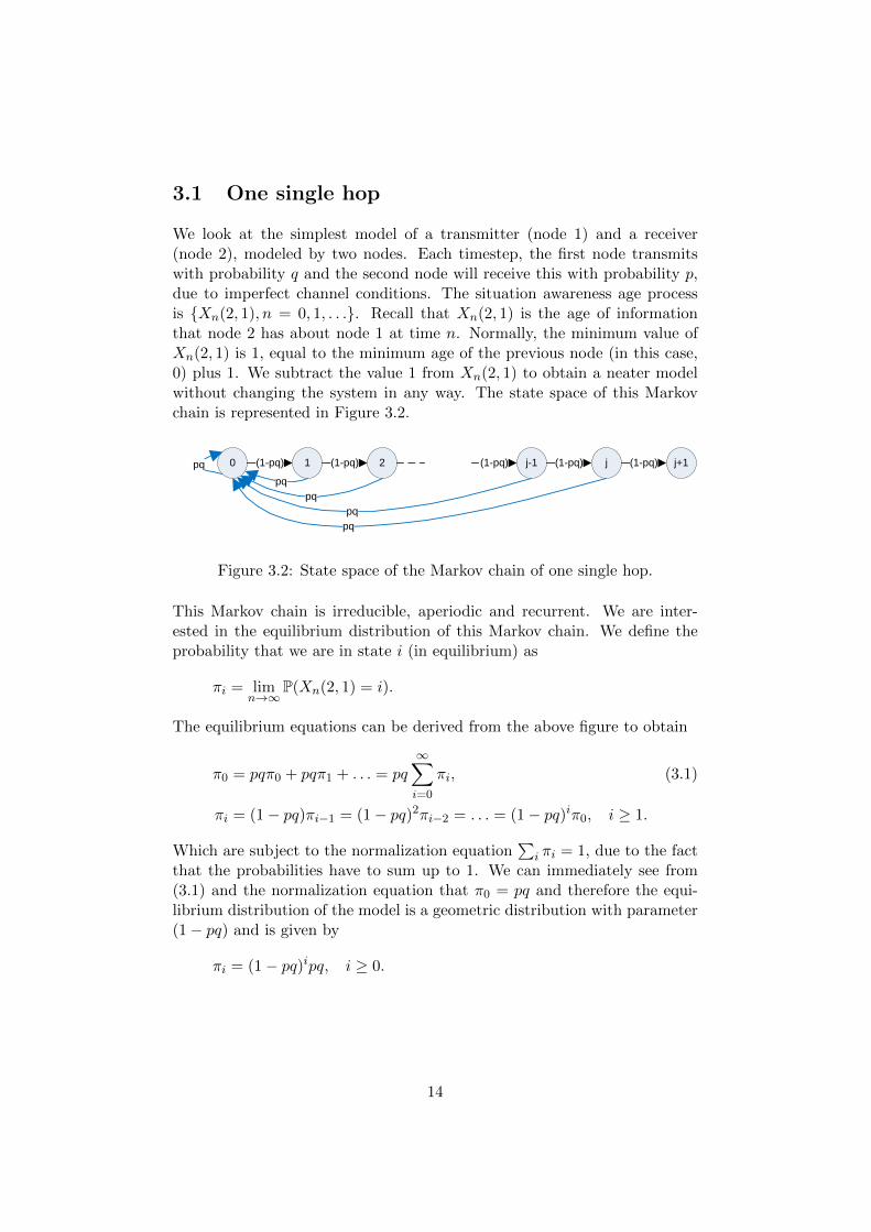
We look at the simplest model of a transmitter (node 1) and a receiver(node 2), modeled by two nodes. Each timestep, the first node transmitswith probability q and the second node will receive this with probability p,due to imperfect channel conditions. The situation awareness age processis {Xn(2, 1), n = 0, 1, . . .}. Recall that Xn(2, 1) is the age of informationthat node 2 has about node 1 at time n. Normally, the minimum value ofXn(2, 1) is 1, equal to the minimum age of the previous node (in this case,0) plus 1. We subtract the value 1 from Xn(2, 1) to obtain a neater modelwithout changing the system in any way. The state space of this Markovchain is represented in Figure 3.2.
0 1 2 j-1 j j+1(1-pq) (1-pq) (1-pq) (1-pq)
pq
pq
pq
pq
pq (1-pq)
Figure 3.2: State space of the Markov chain of one single hop.
This Markov chain is irreducible, aperiodic and recurrent. We are inter-ested in the equilibrium distribution of this Markov chain. We define theprobability that we are in state i (in equilibrium) as
πi = limn→∞
P(Xn(2, 1) = i).
The equilibrium equations can be derived from the above figure to obtain
π0 = pqπ0 + pqπ1 + . . . = pq∞∑i=0
πi, (3.1)
πi = (1− pq)πi−1 = (1− pq)2πi−2 = . . . = (1− pq)iπ0, i ≥ 1.
Which are subject to the normalization equation∑
i πi = 1, due to the factthat the probabilities have to sum up to 1. We can immediately see from(3.1) and the normalization equation that π0 = pq and therefore the equi-librium distribution of the model is a geometric distribution with parameter(1− pq) and is given by
πi = (1− pq)ipq, i ≥ 0.
14
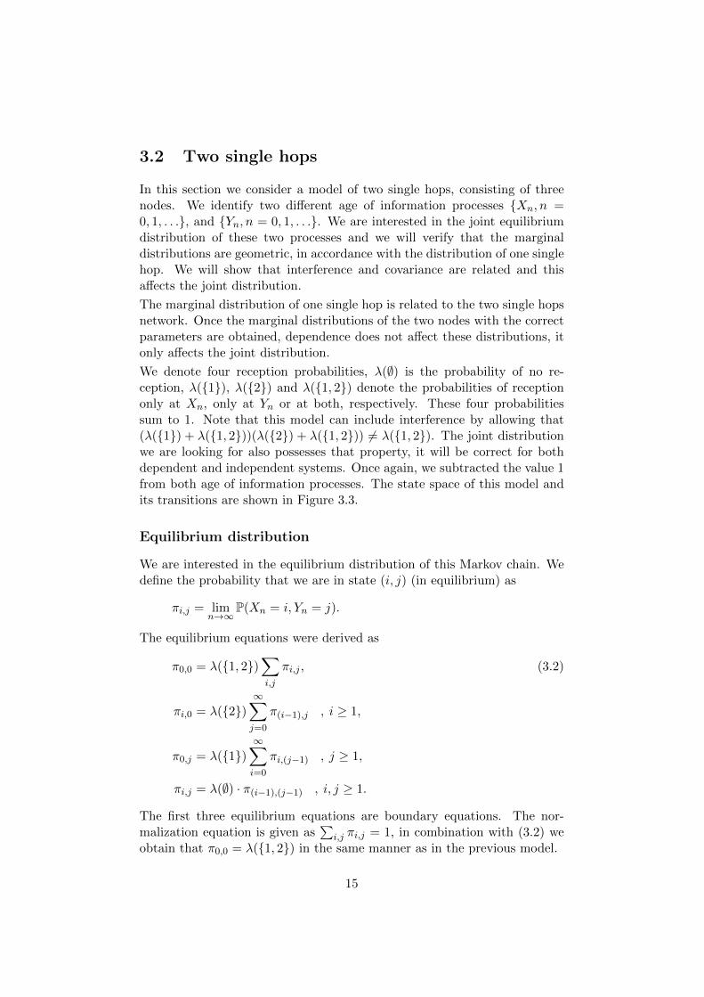
3.2 Two single hops
In this section we consider a model of two single hops, consisting of threenodes. We identify two different age of information processes {Xn, n =0, 1, . . .}, and {Yn, n = 0, 1, . . .}. We are interested in the joint equilibriumdistribution of these two processes and we will verify that the marginaldistributions are geometric, in accordance with the distribution of one singlehop. We will show that interference and covariance are related and thisaffects the joint distribution.
The marginal distribution of one single hop is related to the two single hopsnetwork. Once the marginal distributions of the two nodes with the correctparameters are obtained, dependence does not affect these distributions, itonly affects the joint distribution.
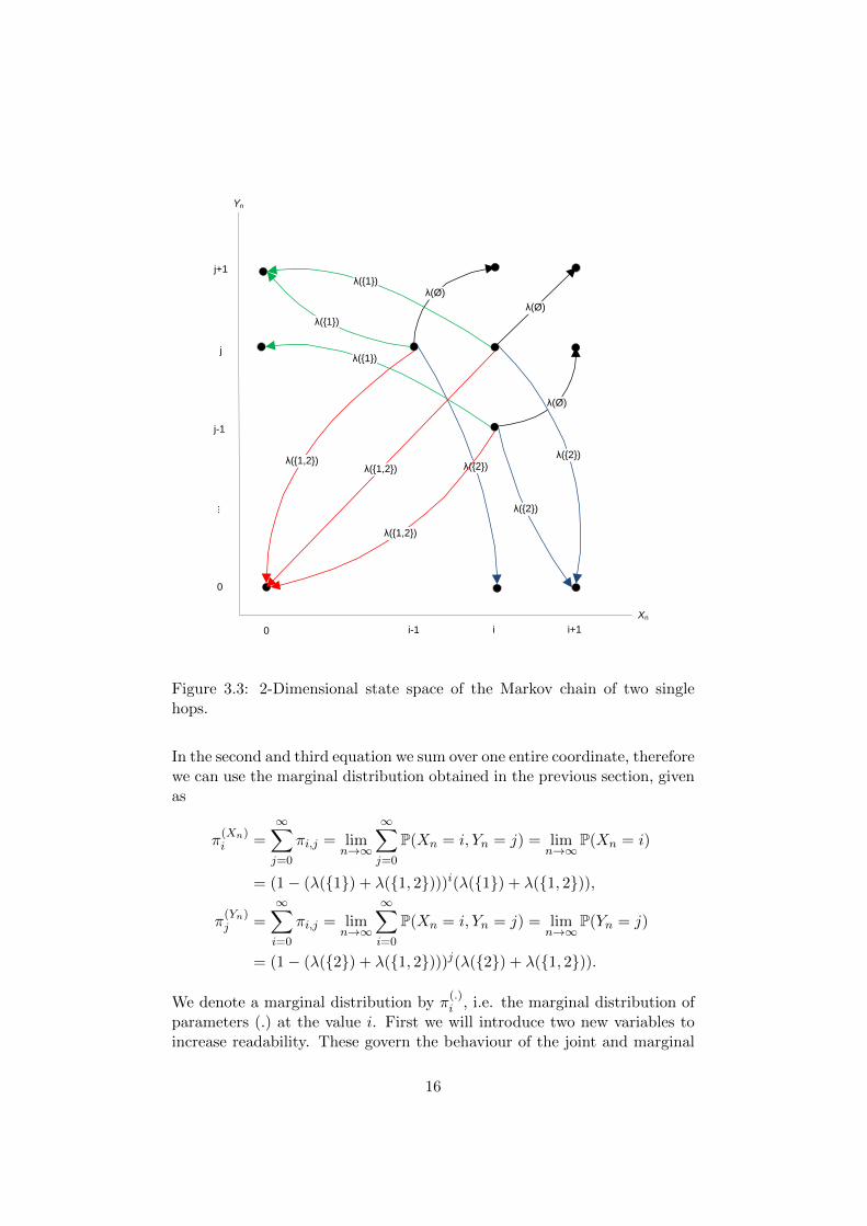
We denote four reception probabilities, λ(∅) is the probability of no re-ception, λ({1}), λ({2}) and λ({1, 2}) denote the probabilities of receptiononly at Xn, only at Yn or at both, respectively. These four probabilitiessum to 1. Note that this model can include interference by allowing that(λ({1}) + λ({1, 2}))(λ({2}) + λ({1, 2})) 6= λ({1, 2}). The joint distributionwe are looking for also possesses that property, it will be correct for bothdependent and independent systems. Once again, we subtracted the value 1from both age of information processes. The state space of this model andits transitions are shown in Figure 3.3.
Equilibrium distribution
We are interested in the equilibrium distribution of this Markov chain. Wedefine the probability that we are in state (i, j) (in equilibrium) as
πi,j = limn→∞
P(Xn = i, Yn = j).
The equilibrium equations were derived as
π0,0 = λ({1, 2})∑i,j
πi,j , (3.2)
πi,0 = λ({2})∞∑j=0
π(i−1),j , i ≥ 1,
π0,j = λ({1})∞∑i=0
πi,(j−1) , j ≥ 1,
πi,j = λ(∅) · π(i−1),(j−1) , i, j ≥ 1.
The first three equilibrium equations are boundary equations. The nor-malization equation is given as
∑i,j πi,j = 1, in combination with (3.2) we
obtain that π0,0 = λ({1, 2}) in the same manner as in the previous model.
15
Xn
Yn
0 ii-1
0
j-1
j
i+1
j+1
λ(Ø)
λ({2})
λ(Ø)
λ(Ø)
λ({2})λ({2})
λ({1})
λ({1})
λ({1})
λ({1,2})λ({1,2})
λ({1,2})
...
Figure 3.3: 2-Dimensional state space of the Markov chain of two singlehops.
In the second and third equation we sum over one entire coordinate, thereforewe can use the marginal distribution obtained in the previous section, givenas
π(Xn)i =
∞∑j=0
πi,j = limn→∞
∞∑j=0
P(Xn = i, Yn = j) = limn→∞
P(Xn = i)
= (1− (λ({1}) + λ({1, 2})))i(λ({1}) + λ({1, 2})),
π(Yn)j =
∞∑i=0
πi,j = limn→∞
∞∑i=0
P(Xn = i, Yn = j) = limn→∞
P(Yn = j)
= (1− (λ({2}) + λ({1, 2})))j(λ({2}) + λ({1, 2})).
We denote a marginal distribution by π(.)i , i.e. the marginal distribution of
parameters (.) at the value i. First we will introduce two new variables toincrease readability. These govern the behaviour of the joint and marginal
16
distributions
c1 = 1− (λ({2}) + λ({1, 2})),c2 = 1− (λ({1}) + λ({1, 2})).
The physical interpretation of these variables is that c1 the probability ofhaving no reception on the second node, and c2 is the probability of having noreception on the first node. Using these two new variables and the marginaldistributions, the equilibrium equations simplify to
π0,0 = λ({1, 2}),
πi,0 = λ({2})π(Xn)i−1 = λ({2})ci−12 (1− c2) , i ≥ 1,
π0,j = λ({1})π(Yn)j−1 = λ({1})cj−11 (1− c1) , j ≥ 1,
πi,j = λ(∅) · π(i−1),(j−1) , i, j ≥ 1.
This can be rewritten to obtain a general geometric formula over the diag-onals
πi,j =
λ(∅)iλ({1, 2}) for i = j,
λ(∅)jλ({2})ci−j−12 (1− c2) for i > j,
λ(∅)iλ({1})cj−i−11 (1− c1) for i < j.
(3.3)
Marginal distribution from the joint distribution
As a sanity check, we will show that the joint distribution indeed possessesthe two marginal distributions we used earlier. We can obtain the marginalof Xn by summing over the Yn coordinate, namely j. The state space alongthis line is partitioned into three sets, as the expression for πi,j also consistsof three parts.
π(Xn)i =
∞∑j=0
πi,j =i−1∑j=0
πi,j + πi,i +∞∑
j=i+1
πi,j
= λ({2})(1− c2)i−1∑j=0
ci−12
(λ(∅)c2
)j+ λ(∅)iλ({1, 2})
+ λ(∅)iλ({1})∞∑
j=i+1
(1− c1)c−(i+1)1 cj1
= (1− c2)(ci2 − λ(∅)i) + λ(∅)iλ({1, 2}) + λ(∅)iλ({1}) = (1− c2)ci2.
The marginal distribution of Xn is, as expected, a geometric distributionwith parameter c2. Note that no assumptions were made on interference ordependence, Xn and Yn could be dependent, yet still the same geometricmarginal distribution is obtained. Similar to the derivation of the marginaldistribution for Xn, we can derive the expression for Yn and find that isgeometric with parameter c1.
17
Interference and covariance
A measure of the dependence is the covariance between the two variables Xand Y (the subscript n is omitted for clarity). It is defined as
Cov(X,Y ) = E((X − E(X))(Y − E(Y )))
= E(XY −XE(Y )− Y E(X) + E(X)E(Y ))
= E(XY )− E(X)E(Y ). (3.4)
Independent variables X and Y ensure the covariance is zero. However, acovariance of zero does not mean that the two variables are independent,it is a one-way relation. The expected value of the joint and the marginaldistributions are needed to calculate the covariance. See Appendix A forthe derivations. The covariance is symmetric and can then be expressed as
Cov(X,Y ) =λ(∅)λ({1, 2})− λ({1})λ({2})
(λ({1}) + λ({1, 2}))(λ({2}) + λ({1, 2}))(1− λ(∅)).
If there is no interference between the two transmitters, the covariance has tobe equal to 0 and the joint distribution is the product of the two marginal dis-
tributions, πi,j = π(X)i π
(Y )j . For no interference (λ({1})+λ({1, 2}))(λ({2})+
λ({1, 2})) = λ({1, 2}) has to hold, meaning that the probability of recep-tion of both is the product of the (independent) probability that one ofthem receives. As this is a quadratic equation, there are two possible val-ues for λ({1, 2}) that satisfy this equation. These two values that satisfythe previous equation, are also the only two values for λ({1, 2}) that satisfyCov(X,Y ) = 0. We deduced that in the independent case one of the twogave an infeasible result and thus we can conclude that the value
λ({1, 2}) =1
2
(((λ({1})− λ({2})
)2− 2λ({1})− 2λ({2}) + 1
) 12
+ (1− λ({1})− λ({2})))
(3.5)
is the parameter value that sets the covariance equal to 0 and the jointdistribution is the product of the two marginal distributions. The infeasibleresult for λ({1, 2}) indeed does not give a joint distribution that is theproduct of the two marginal distributions. We can conclude that if andonly if (3.5) holds, the joint distribution is the product of the two marginaldistributions.
18
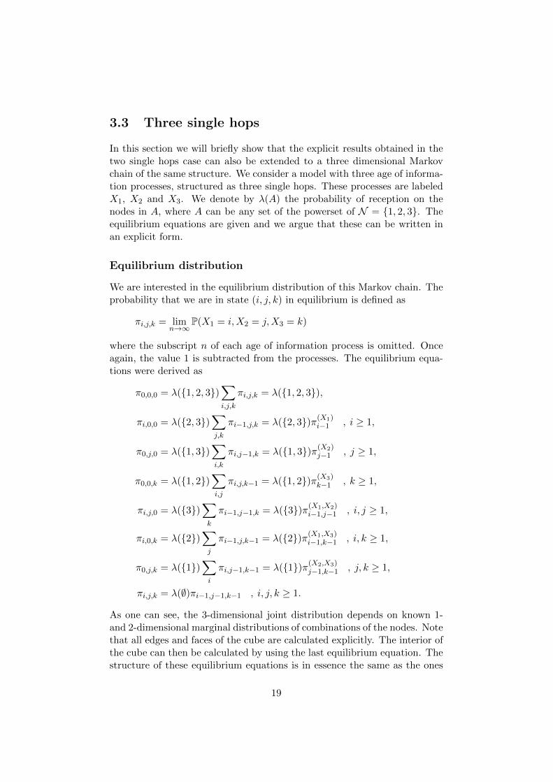
3.3 Three single hops
In this section we will briefly show that the explicit results obtained in thetwo single hops case can also be extended to a three dimensional Markovchain of the same structure. We consider a model with three age of informa-tion processes, structured as three single hops. These processes are labeledX1, X2 and X3. We denote by λ(A) the probability of reception on thenodes in A, where A can be any set of the powerset of N = {1, 2, 3}. Theequilibrium equations are given and we argue that these can be written inan explicit form.
Equilibrium distribution
We are interested in the equilibrium distribution of this Markov chain. Theprobability that we are in state (i, j, k) in equilibrium is defined as
πi,j,k = limn→∞
P(X1 = i,X2 = j,X3 = k)
where the subscript n of each age of information process is omitted. Onceagain, the value 1 is subtracted from the processes. The equilibrium equa-tions were derived as
π0,0,0 = λ({1, 2, 3})∑i,j,k
πi,j,k = λ({1, 2, 3}),
πi,0,0 = λ({2, 3})∑j,k
πi−1,j,k = λ({2, 3})π(X1)i−1 , i ≥ 1,
π0,j,0 = λ({1, 3})∑i,k
πi,j−1,k = λ({1, 3})π(X2)j−1 , j ≥ 1,
π0,0,k = λ({1, 2})∑i,j
πi,j,k−1 = λ({1, 2})π(X3)k−1 , k ≥ 1,
πi,j,0 = λ({3})∑k
πi−1,j−1,k = λ({3})π(X1,X2)i−1,j−1 , i, j ≥ 1,
πi,0,k = λ({2})∑j
πi−1,j,k−1 = λ({2})π(X1,X3)i−1,k−1 , i, k ≥ 1,
π0,j,k = λ({1})∑i
πi,j−1,k−1 = λ({1})π(X2,X3)j−1,k−1 , j, k ≥ 1,
πi,j,k = λ(∅)πi−1,j−1,k−1 , i, j, k ≥ 1.
As one can see, the 3-dimensional joint distribution depends on known 1-and 2-dimensional marginal distributions of combinations of the nodes. Notethat all edges and faces of the cube are calculated explicitly. The interior ofthe cube can then be calculated by using the last equilibrium equation. Thestructure of these equilibrium equations is in essence the same as the ones
19
obtained from the two single hops case. In that 2-dimensional Markov chainthe edges are known explicitly and the interior is computed from these edges.Thus, using the same methodology a general geometric expression over thediagonals can be obtained. One can split the state space into 13 subsets, inthe same manner the formula for πi,j was split into three parts. We refrainfrom deriving these subsets and their corresponding explicit expressions asthere is little gain in showing them after it was derived that such explicitformulaes exist.
20
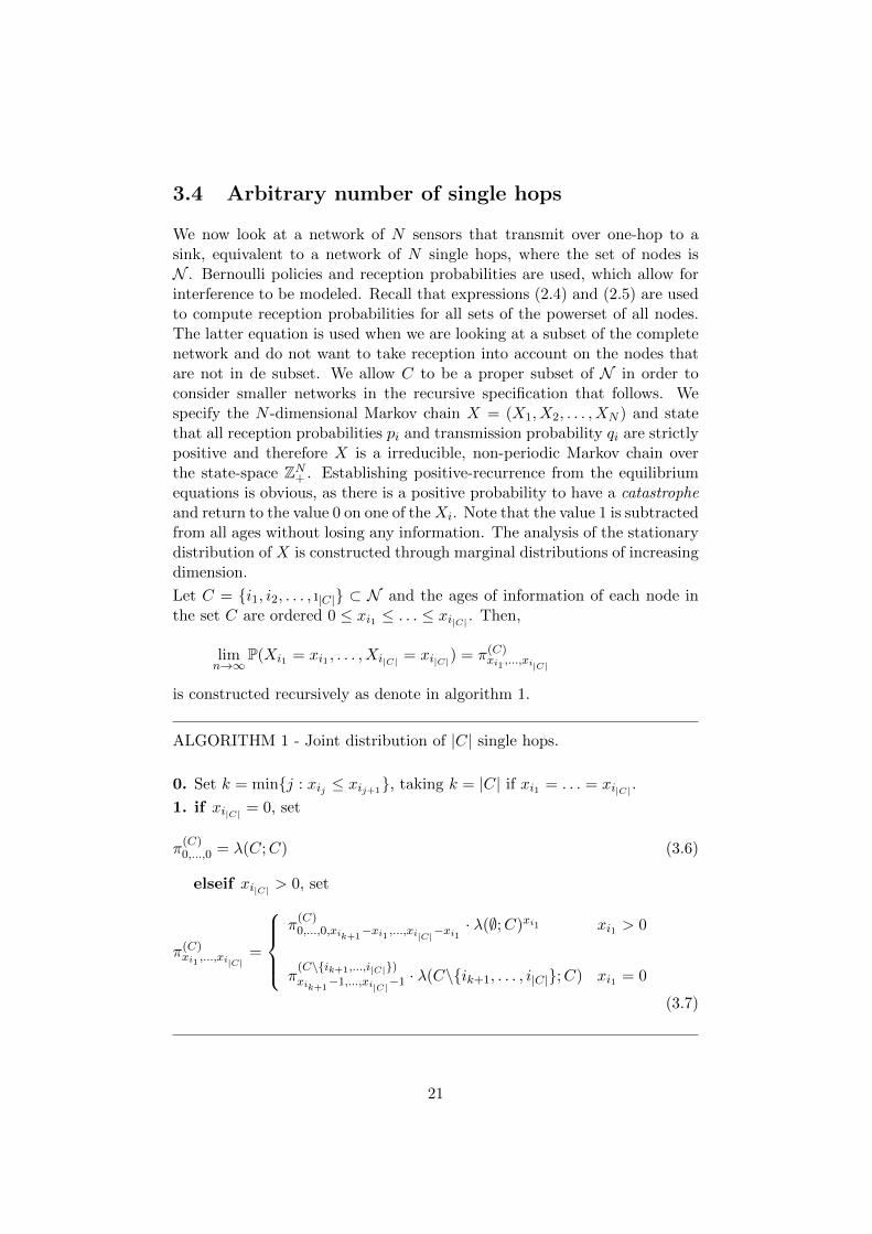
3.4 Arbitrary number of single hops
We now look at a network of N sensors that transmit over one-hop to asink, equivalent to a network of N single hops, where the set of nodes isN . Bernoulli policies and reception probabilities are used, which allow forinterference to be modeled. Recall that expressions (2.4) and (2.5) are usedto compute reception probabilities for all sets of the powerset of all nodes.The latter equation is used when we are looking at a subset of the completenetwork and do not want to take reception into account on the nodes thatare not in de subset. We allow C to be a proper subset of N in order toconsider smaller networks in the recursive specification that follows. Wespecify the N -dimensional Markov chain X = (X1, X2, . . . , XN ) and statethat all reception probabilities pi and transmission probability qi are strictlypositive and therefore X is a irreducible, non-periodic Markov chain overthe state-space ZN+ . Establishing positive-recurrence from the equilibriumequations is obvious, as there is a positive probability to have a catastropheand return to the value 0 on one of theXi. Note that the value 1 is subtractedfrom all ages without losing any information. The analysis of the stationarydistribution of X is constructed through marginal distributions of increasingdimension.
Let C = {i1, i2, . . . , ı|C|} ⊂ N and the ages of information of each node inthe set C are ordered 0 ≤ xi1 ≤ . . . ≤ xi|C| . Then,
limn→∞
P(Xi1 = xi1 , . . . , Xi|C| = xi|C|) = π(C)xi1 ,...,xi|C|
is constructed recursively as denote in algorithm 1.
ALGORITHM 1 - Joint distribution of |C| single hops.
0. Set k = min{j : xij ≤ xij+1}, taking k = |C| if xi1 = . . . = xi|C| .
1. if xi|C| = 0, set
π(C)0,...,0 = λ(C;C) (3.6)
elseif xi|C| > 0, set
π(C)xi1 ,...,xi|C|
=
π(C)0,...,0,xik+1
−xi1 ,...,xi|C|−xi1· λ(∅;C)xi1 xi1 > 0
π(C\{ik+1,...,i|C|})xik+1
−1,...,xi|C|−1· λ(C\{ik+1, . . . , i|C|};C) xi1 = 0
(3.7)
21
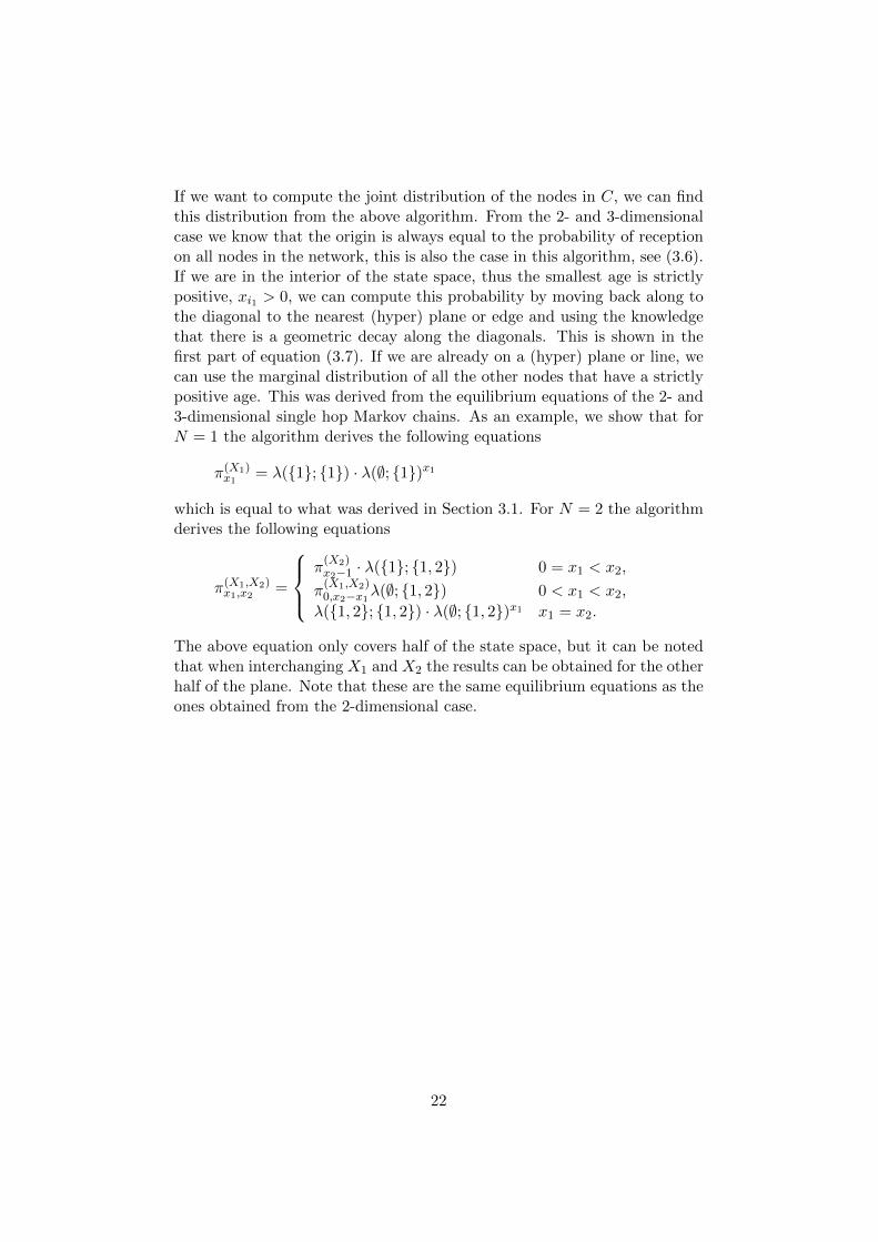
If we want to compute the joint distribution of the nodes in C, we can findthis distribution from the above algorithm. From the 2- and 3-dimensionalcase we know that the origin is always equal to the probability of receptionon all nodes in the network, this is also the case in this algorithm, see (3.6).If we are in the interior of the state space, thus the smallest age is strictlypositive, xi1 > 0, we can compute this probability by moving back along tothe diagonal to the nearest (hyper) plane or edge and using the knowledgethat there is a geometric decay along the diagonals. This is shown in thefirst part of equation (3.7). If we are already on a (hyper) plane or line, wecan use the marginal distribution of all the other nodes that have a strictlypositive age. This was derived from the equilibrium equations of the 2- and3-dimensional single hop Markov chains. As an example, we show that forN = 1 the algorithm derives the following equations
π(X1)x1 = λ({1}; {1}) · λ(∅; {1})x1
which is equal to what was derived in Section 3.1. For N = 2 the algorithmderives the following equations
π(X1,X2)x1,x2 =
π(X2)x2−1 · λ({1}; {1, 2}) 0 = x1 < x2,
π(X1,X2)0,x2−x1λ(∅; {1, 2}) 0 < x1 < x2,
λ({1, 2}; {1, 2}) · λ(∅; {1, 2})x1 x1 = x2.
The above equation only covers half of the state space, but it can be notedthat when interchanging X1 and X2 the results can be obtained for the otherhalf of the plane. Note that these are the same equilibrium equations as theones obtained from the 2-dimensional case.
22
3.5 Minimum over a joint distribution of a singlehop network
Once one has obtained the joint distribution of the nodes that are withina sink, e.g. think of the second type of single hop network in Figure 3.1,where all sources share the same sensing information from a sensor, theminimum has to be taken to get the marginal distribution of the sink. Thisphenomenon is explained by the fact that a node always wants the mostupdated information and if it receives from two previous at the same time,it will only take the most up-to-date information. The minimum in a discretestate space can be computed by setting one of the ages to a specific valueand summing over all larger values in the other dimensions. Setting an ageto a specific value should be done for all dimensions and the minimum forthat specific value is then equal to the summation of the computed sums.One should note not to count any state more than once. An example istreated to illustrate the above explanation.
We consider the two single hops network of Section 3.2. Recall that thereare two age of information processes Xn and Yn (with the value 1 subtractedfrom their ages), if we consider these to be part of the sink we can take theminimum to obtain the marginal distribution, let us define the correspondingstochastic variable as
Zn = min(Xn, Yn).
We are interested in π(Z)z = limn→∞ P(Zn = z), the equilibrium distribution
of Zn. The minimum over the 2-dimensional Markov chain can be computedby summing over 2 lines.
The computation of the equilibrium distribution can be expressed as
π(Z)z = limn→∞
( ∞∑k=1
P(Xn = z, Yn = z + k)
+
∞∑k=1
P(Xn = z + k, Yn = z) + P(Xn = z, Yn = z)
)
=
∞∑k=1
πz,z+k +
∞∑k=1
πz+k,z + πz,z.
If we now use the derived expressions for πi,j , the above computation can
23
be expressed as
π(Z)z = λ(∅)zλ({1})(1− c1)∞∑k=0
ck1 + λ(∅)zλ({2})(1− c2)∞∑k=0
ck2
+ λ(∅)zλ({1, 2})= λ(∅)z (λ({1}) + λ({2}) + λ({1, 2}))= λ(∅)z(1− λ(∅)).
We can conclude that for two geometric stochastic variables and any depen-dence structure, the minimum of these two variables also has a geometricdistribution. The interference can also be found in the above expression, asλ(∅) is larger when there is interference and more probability mass is presentat higher levels.
The same methodology can be applied to an N -dimensional Markov chainsas long as their joint distribution is known.
Chapter summary
In this chapter we studied the single hop networks and finally we were ableto derive an algorithm that computes the joint distribution of an arbitrarynumber of single hops. The 2-dimensional case was analyzed in greater detailand it was found that the joint distribution is the product of its marginaldistribution for one value of λ({1, 2}). The chapter was concluded with anexplanation on how to obtain the marginal distribution of a sink. In thenext chapter a line of relays is studied and an algorithm is derived thatiteratively computes joint distributions of two succeeding nodes.
24
Chapter 4
Line of relays
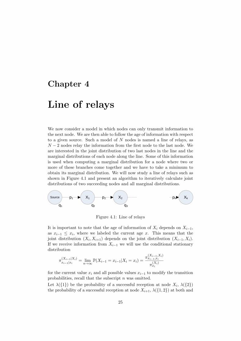
We now consider a model in which nodes can only transmit information tothe next node. We are then able to follow the age of information with respectto a given source. Such a model of N nodes is named a line of relays, asN − 2 nodes relay the information from the first node to the last node. Weare interested in the joint distribution of two last nodes in the line and themarginal distributions of each node along the line. Some of this informationis used when computing a marginal distribution for a node where two ormore of these branches come together and we have to take a minimum toobtain its marginal distribution. We will now study a line of relays such asshown in Figure 4.1 and present an algorithm to iteratively calculate jointdistributions of two succeeding nodes and all marginal distributions.
Source X1 X2 Xkp1 p2 pk
q1 q2 q3
Figure 4.1: Line of relays
It is important to note that the age of information of Xi depends on Xi−1,as xi−1 ≤ xi, where we labeled the current age x. This means that thejoint distribution (Xi, Xi+1) depends on the joint distribution (Xi−1, Xi).If we receive information from Xi−1 we will use the conditional stationarydistribution
π(Xi−1|Xi)xi−1|xi = lim
n→∞P(Xi−1 = xi−1|Xi = xi) =
π(Xi−1,Xi)xi−1,xi
π(Xi)xi
for the current value xi and all possible values xi−1 to modify the transitionprobabilities, recall that the subscript n was omitted.
Let λ({1}) be the probability of a successful reception at node Xi, λ({2})the probability of a successful reception at node Xi+1, λ({1, 2}) at both and
25
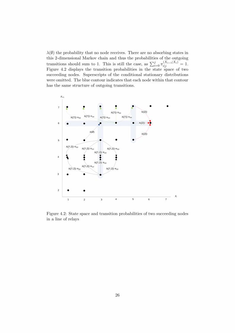
λ(∅) the probability that no node receives. There are no absorbing states inthis 2-dimensional Markov chain and thus the probabilities of the outgoing
transitions should sum to 1. This is still the case, as∑j
i=0 π(Xi−1|Xi)i|j = 1.
Figure 4.2 displays the transition probabilities in the state space of twosucceeding nodes. Superscripts of the conditional stationary distributionswere omitted. The blue contour indicates that each node within that contourhas the same structure of outgoing transitions.
Xi
Xi+1
1 43
2
4
5
5
6
3
2
7
6 7
λ({1,2}) π0|3
λ({1,2}) π1|3
λ({1,2}) π2|3
λ({1,2}) π3|3
λ({1}) π0|4λ({1}) π1|4 λ({1}) π2|4
λ({1}) π3|4
λ({2})
λ({2})
λ({2})
λ(Ø)
λ({1}) π4|4
λ({1,2}) π0|3λ({1,2}) π1|3
λ({1,2}) π2|3
λ({1,2}) π3|3
Figure 4.2: State space and transition probabilities of two succeeding nodesin a line of relays
26
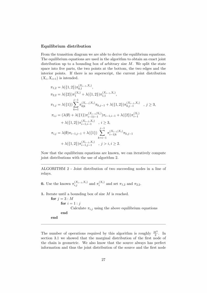
Equilibrium distribution
From the transition diagram we are able to derive the equilibrium equations.The equilibrium equations are used in the algorithm to obtain an exact jointdistribution up to a bounding box of arbitrary size M . We split the statespace into five parts, the two points at the bottom, the two edges and theinterior points. If there is no superscript, the current joint distribution(Xi, Xi+1) is intended.
π1,2 = λ({1, 2})π(Xi−1,Xi)0,1 ,
π2,2 = λ({2})π(Xi)1 + λ({1, 2})π(Xi−1,Xi)
1,1 ,
π1,j = λ({1})j−1∑k=1
π(Xi−1|Xi)0|k πk,j−1 + λ({1, 2})π(Xi−1,Xi)
0,j−1 , j ≥ 3,
πi,i = (λ(∅) + λ({1})π(Xi−1|Xi)i−1|i−1 )πi−1,i−1 + λ({2})π(Xi)
i−1
+ λ({1, 2})π(Xi−1,Xi)i−1,i−1 , i ≥ 3,
πi,j = λ(∅)πi−1,j−1 + λ({1})j−1∑k=i−1
π(Xi−1|Xi)i−1|k πk,j−1
+ λ({1, 2})π(Xi−1,Xi)i−1,j−1 , j > i, i ≥ 2.
Now that the equilibrium equations are known, we can iteratively computejoint distributions with the use of algorithm 2.
ALGORITHM 2 - Joint distribution of two succeeding nodes in a line ofrelays.
0. Use the known π(Xi−1,Xi)i,j and π
(Xi)i and set π1,2 and π2,2.
1. Iterate until a bounding box of size M is reached.for j = 3 : M
for i = 1 : jCalculate πi,j using the above equilibrium equations
endend
The number of operations required by this algorithm is roughly M2
2 . Insection 3.1 we showed that the marginal distribution of the first node ofthe chain is geometric. We also know that the source always has perfectinformation and thus the joint distribution of the source and the first node
27
is exactly the geometric distribution along the axis where the age of infor-mation of the source is 0. Supplying this joint and marginal distribution tothe algorithm allows us to calculate all joint distributions of two succeedingnodes of a line of relays.
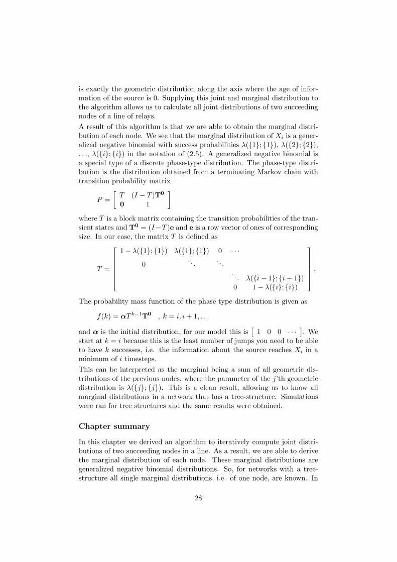
A result of this algorithm is that we are able to obtain the marginal distri-bution of each node. We see that the marginal distribution of Xi is a gener-alized negative binomial with success probabilities λ({1}; {1}), λ({2}; {2}),. . ., λ({i}; {i}) in the notation of (2.5). A generalized negative binomial isa special type of a discrete phase-type distribution. The phase-type distri-bution is the distribution obtained from a terminating Markov chain withtransition probability matrix
P =
[T (I − T )T0
0 1
]where T is a block matrix containing the transition probabilities of the tran-sient states and T0 = (I−T )e and e is a row vector of ones of correspondingsize. In our case, the matrix T is defined as
T =
1− λ({1}; {1}) λ({1}; {1}) 0 · · ·
0. . .
. . .
. . . λ({i− 1}; {i− 1})0 1− λ({i}; {i})
.The probability mass function of the phase type distribution is given as
f(k) = αT k−1T0 , k = i, i+ 1, . . .
and α is the initial distribution, for our model this is[
1 0 0 · · ·]. We
start at k = i because this is the least number of jumps you need to be ableto have k successes, i.e. the information about the source reaches Xi in aminimum of i timesteps.
This can be interpreted as the marginal being a sum of all geometric dis-tributions of the previous nodes, where the parameter of the j’th geometricdistribution is λ({j}; {j}). This is a clean result, allowing us to know allmarginal distributions in a network that has a tree-structure. Simulationswere ran for tree structures and the same results were obtained.
Chapter summary
In this chapter we derived an algorithm to iteratively compute joint distri-butions of two succeeding nodes in a line. As a result, we are able to derivethe marginal distribution of each node. These marginal distributions aregeneralized negative binomial distributions. So, for networks with a tree-structure all single marginal distributions, i.e. of one node, are known. In
28

the next chapter we will analyze a network with two branches, where we usethe knowledge obtained in the previous chapters.
29

Chapter 5
A network with two branches
In the previous two chapters we derived the steady state distributions ofsingle hop networks and the joint distribution of two nodes in a line of relays.We also looked at ways to compute the minimum over a joint distribution oftwo nodes. This knowledge is used in obtaining the distribution of the age ofinformation at a sink given there are two routes from the source to the sink.Note that we deal with a tree structure right up until the point we reachthe sink. Dependence between the links occurs due to the fact that the twobranches are connected at the source, as we have already discovered in thesingle hops network. Interference can still occur between the two branchesor from other nodes in the surrounding network. Figure 5.1 shows the modelwe are describing. The motivation for looking at such a model is the analogywith an intelligent transport system in a city grid, where we want to sendinformation from one intersection to the next intersection through the twoshortest routes.
Source
X11 X12p12
q12 q13
p11
X21 X22p22 p2k
q22 q23
p21
q1
p1k X1k
X2k
Figure 5.1: Two branches of a tree-structured network
The main goal is to be able to iterate over these two branches by continuallycalculating a four dimensional joint distribution, starting at the source. Forthis iteration we first need to gain insight in the three- and four-dimensionaljoint distributions. The first section of this chapter discusses the algorithm
30

and equilibrium equations used to calculate the three-dimensional distri-bution. We continue by showing the four-dimensional case and finally wepresent the main iteration algorithm.
31
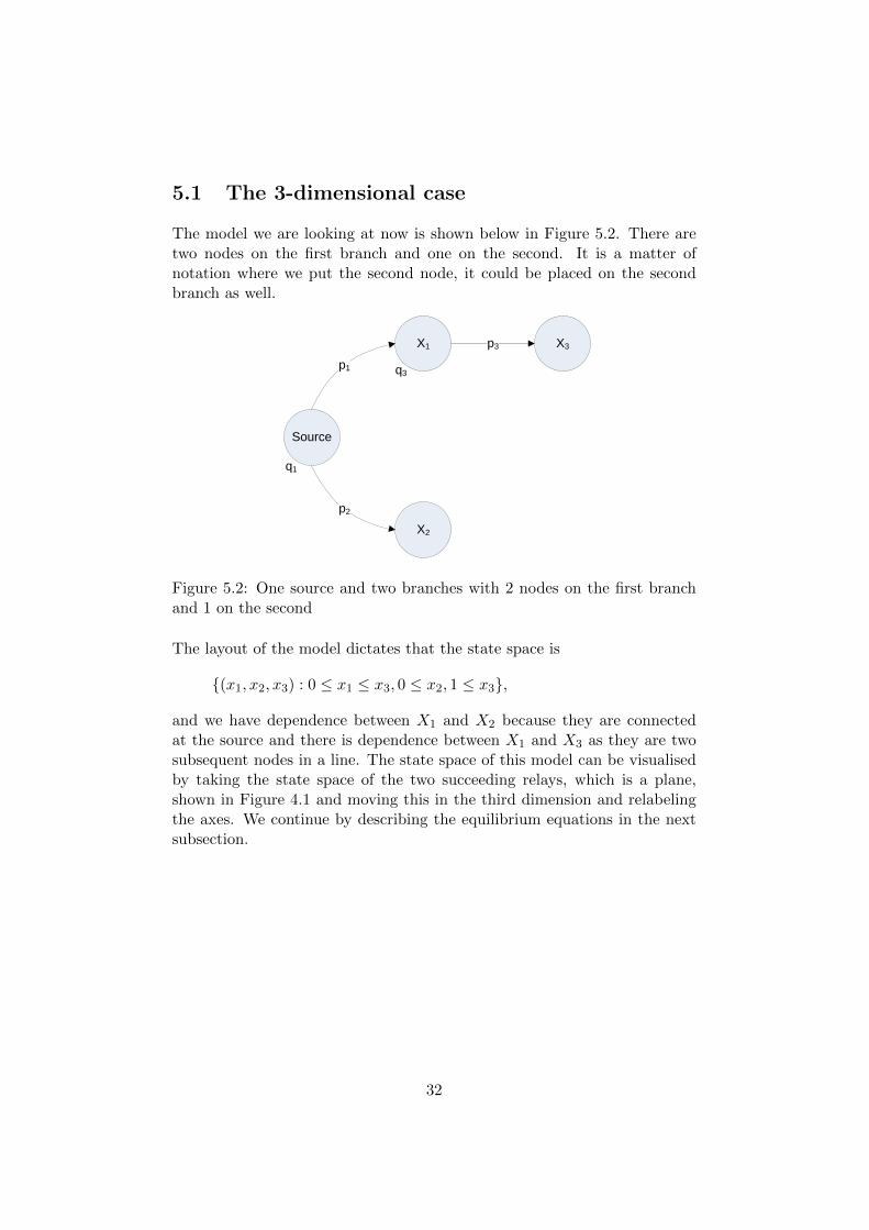
5.1 The 3-dimensional case
The model we are looking at now is shown below in Figure 5.2. There aretwo nodes on the first branch and one on the second. It is a matter ofnotation where we put the second node, it could be placed on the secondbranch as well.
Source
X1
X2
X3
p1
p2
p3
q3
q1
Figure 5.2: One source and two branches with 2 nodes on the first branchand 1 on the second
The layout of the model dictates that the state space is
{(x1, x2, x3) : 0 ≤ x1 ≤ x3, 0 ≤ x2, 1 ≤ x3},
and we have dependence between X1 and X2 because they are connectedat the source and there is dependence between X1 and X3 as they are twosubsequent nodes in a line. The state space of this model can be visualisedby taking the state space of the two succeeding relays, which is a plane,shown in Figure 4.1 and moving this in the third dimension and relabelingthe axes. We continue by describing the equilibrium equations in the nextsubsection.
32
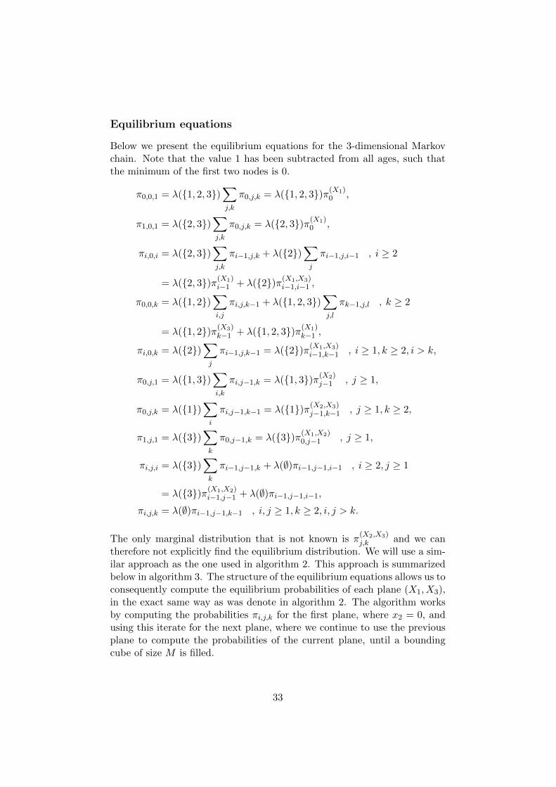
Equilibrium equations
Below we present the equilibrium equations for the 3-dimensional Markovchain. Note that the value 1 has been subtracted from all ages, such thatthe minimum of the first two nodes is 0.
π0,0,1 = λ({1, 2, 3})∑j,k
π0,j,k = λ({1, 2, 3})π(X1)0 ,
π1,0,1 = λ({2, 3})∑j,k
π0,j,k = λ({2, 3})π(X1)0 ,
πi,0,i = λ({2, 3})∑j,k
πi−1,j,k + λ({2})∑j
πi−1,j,i−1 , i ≥ 2
= λ({2, 3})π(X1)i−1 + λ({2})π(X1,X3)
i−1,i−1 ,
π0,0,k = λ({1, 2})∑i,j
πi,j,k−1 + λ({1, 2, 3})∑j,l
πk−1,j,l , k ≥ 2
= λ({1, 2})π(X3)k−1 + λ({1, 2, 3})π(X1)
k−1 ,
πi,0,k = λ({2})∑j
πi−1,j,k−1 = λ({2})π(X1,X3)i−1,k−1 , i ≥ 1, k ≥ 2, i > k,
π0,j,1 = λ({1, 3})∑i,k
πi,j−1,k = λ({1, 3})π(X2)j−1 , j ≥ 1,
π0,j,k = λ({1})∑i
πi,j−1,k−1 = λ({1})π(X2,X3)j−1,k−1 , j ≥ 1, k ≥ 2,
π1,j,1 = λ({3})∑k
π0,j−1,k = λ({3})π(X1,X2)0,j−1 , j ≥ 1,
πi,j,i = λ({3})∑k
πi−1,j−1,k + λ(∅)πi−1,j−1,i−1 , i ≥ 2, j ≥ 1
= λ({3})π(X1,X2)i−1,j−1 + λ(∅)πi−1,j−1,i−1,
πi,j,k = λ(∅)πi−1,j−1,k−1 , i, j ≥ 1, k ≥ 2, i, j > k.
The only marginal distribution that is not known is π(X2,X3)j,k and we can
therefore not explicitly find the equilibrium distribution. We will use a sim-ilar approach as the one used in algorithm 2. This approach is summarizedbelow in algorithm 3. The structure of the equilibrium equations allows us toconsequently compute the equilibrium probabilities of each plane (X1, X3),in the exact same way as was denote in algorithm 2. The algorithm worksby computing the probabilities πi,j,k for the first plane, where x2 = 0, andusing this iterate for the next plane, where we continue to use the previousplane to compute the probabilities of the current plane, until a boundingcube of size M is filled.
33
ALGORITHM 3 - Joint distribution of a network with 2 branches, 2 nodeson the first branch and 1 on the second.
0. Obtain the marginal and joint distributions π(X1,X2)i,j , π
(X1,X3)i,k , π
(X1)i , π
(X2)j
and π(X3)k from earlier results or using algorithm 2 and set π0,0,1 and π1,0,1.
1. Find πi,0,k in the same fashion as algorithm 2, until a bounding box ofsize M is reached.
for k = 2 : Mfor i = 0 : k
Calculate πi,0,kend
end
2. Iterate this plane by increasing j by one each step, until a cube of sizeM is filled.
for j = 1 : MSet π0,j,1 and π1,j,1for k = 2 : M
for i = 0 : kCalculate πi,j,k
endend
end
This algorithm gives us the exact values for πi,j,k up until a bounding cubeof size M . We can validate the joint distribution by comparing it to thejoint distribution of two succeeding nodes in a line by summing out thesingle node on the second branch. Another check that is performed, is ob-taining the marginal for one node from the joint distribution and checkingthis against the generalized negative binomial expression. Both validationchecks hold and the above algorithm has been shown to work correctly.
34
5.2 The 4-dimensional case
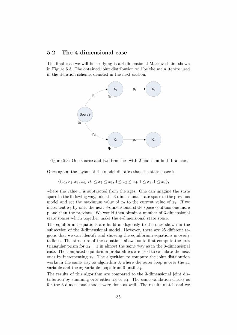
The final case we will be studying is a 4-dimensional Markov chain, shownin Figure 5.3. The obtained joint distribution will be the main iterate usedin the iteration scheme, denoted in the next section.
Source
X1
X2
X3
p1
p2
p3
q3
q1
X4p4
q4
Figure 5.3: One source and two branches with 2 nodes on both branches
Once again, the layout of the model dictates that the state space is
{(x1, x2, x3, x4) : 0 ≤ x1 ≤ x3, 0 ≤ x2 ≤ x4, 1 ≤ x3, 1 ≤ x4},
where the value 1 is subtracted from the ages. One can imagine the statespace in the following way, take the 3-dimensional state space of the previousmodel and set the maximum value of x2 to the current value of x4. If weincrement x4 by one, the next 3-dimensional state space contains one moreplane than the previous. We would then obtain a number of 3-dimensionalstate spaces which together make the 4-dimensional state space.
The equilibrium equations are build analogously to the ones shown in thesubsection of the 3-dimensional model. However, there are 25 different re-gions that we can identify and showing the equilibrium equations is overlytedious. The structure of the equations allows us to first compute the firsttriangular prism for x4 = 1 in almost the same way as in the 3-dimensionalcase. The computed equilibrium probabilities are used to calculate the nextones by incrementing x4. The algorithm to compute the joint distributionworks in the same way as algorithm 3, where the outer loop is over the x4variable and the x2 variable loops from 0 until x4.
The results of this algorithm are compared to the 3-dimensional joint dis-tribution by summing over either x3 or x4. The same validation checks asfor the 3-dimensional model were done as well. The results match and we
35

conclude that this algorithm is successful. In the next section we will usethe obtained knowledge on 3- and 4-dimensional joint distributions, togetherwith the conditioning used for the two succeeding relays, to iterate the latterdistribution over a tree network with two branches.
36
5.3 Iterating over two branches
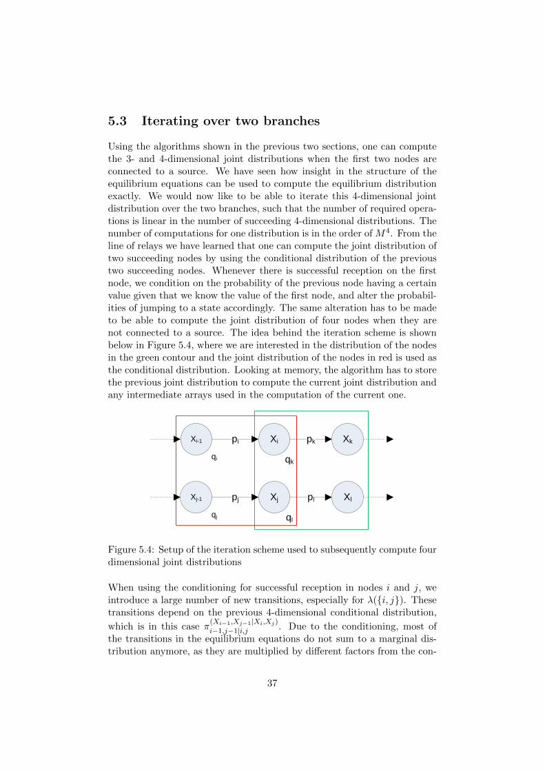
Using the algorithms shown in the previous two sections, one can computethe 3- and 4-dimensional joint distributions when the first two nodes areconnected to a source. We have seen how insight in the structure of theequilibrium equations can be used to compute the equilibrium distributionexactly. We would now like to be able to iterate this 4-dimensional jointdistribution over the two branches, such that the number of required opera-tions is linear in the number of succeeding 4-dimensional distributions. Thenumber of computations for one distribution is in the order of M4. From theline of relays we have learned that one can compute the joint distribution oftwo succeeding nodes by using the conditional distribution of the previoustwo succeeding nodes. Whenever there is successful reception on the firstnode, we condition on the probability of the previous node having a certainvalue given that we know the value of the first node, and alter the probabil-ities of jumping to a state accordingly. The same alteration has to be madeto be able to compute the joint distribution of four nodes when they arenot connected to a source. The idea behind the iteration scheme is shownbelow in Figure 5.4, where we are interested in the distribution of the nodesin the green contour and the joint distribution of the nodes in red is used asthe conditional distribution. Looking at memory, the algorithm has to storethe previous joint distribution to compute the current joint distribution andany intermediate arrays used in the computation of the current one.
Xi-1 Xi Xkpi
qi qk
Xj-1 Xj Xlpj
qj ql
pk
pl
Figure 5.4: Setup of the iteration scheme used to subsequently compute fourdimensional joint distributions
When using the conditioning for successful reception in nodes i and j, weintroduce a large number of new transitions, especially for λ({i, j}). Thesetransitions depend on the previous 4-dimensional conditional distribution,
which is in this case π(Xi−1,Xj−1|Xi,Xj)
i−1,j−1|i,j . Due to the conditioning, most ofthe transitions in the equilibrium equations do not sum to a marginal dis-tribution anymore, as they are multiplied by different factors from the con-
37
ditional distribution. Therefore, equilibrium equations usually depend on alarge subset of the state space and there is no neat structure that can beexploited with a previously obtained algorithm such as algorithm 3. Mostof the points in the state space have incoming transitions from states veryfar away, which cannot be summed to a marginal distribution. Truncationhas to be used at a level M to be able to get a joint distribution. Then weare able to construct a system of linear equations that is of the form
Ax = b
where x is a lexicographical ordering of the state,
x = [π0,0,1,1, π0,1,1,1, . . . , π0,M,1,1, π1,0,1,1, . . . , πM,M,1,1, π0,0,2,1, . . . ,
πM,M,M,1, π0,0,1,2, . . .].
Each row of the matrix A is an equilibrium equation, note that some rowsexplicitly state that a value πi,j,k,l = 0, as they are outside the feasible statespace domain. One would expect the vector b only has zeros, as we aredealing with a Markov chain. This is not the case for this system. If wehave reception on nodes k and/or l, we can sum out this variable and weare left with a marginal distribution of nodes i, j and possibly node k orl that did not receive a packet. These marginal distributions can be com-puted beforehand and supplied to the algorithm that constructs the A andb matrices, such that they end up on the right hand side of the equation.Hence, the vector b has non-zero elements and using normalization is notnecessary; increasing the size of the bounding box will ensure the summationover the equilibrium probabilities converges to 1, and thus the approximatesolution converges to the exact solution. The M-file that computes eachiterate can be found in Appendix C and the main M-file for running theiteration scheme can be found in Appendix D. In the next subsection weaddress memory and time constraint problems we encountered, the subsec-tion after that validates the proposed iteration scheme and M-file. The finalsubsection concludes with some remarks on the length of the two branches.
Memory and time constraints
In the iteration scheme we are dealing with a joint distribution of length Min all four dimensions. This leads to an A matrix of size M4-by-M4. For amoderate value for M , a full matrix would lead to out of memory errors ona 2 GB RAM system. We therefore need to gain insight into how Matlabhandles memory and study the algorithm, as initially, the computation ofone iterate would take 18 hours on an Intel Dual Core T7200 2.00 GHzlaptop. We use [6] as a guide to the optimization.
Matlab uses copy on write, which means that in an assignment of one vari-able to the other, it only passes a pointer as long as the data is unaltered.
38

Once we change the contents, it copies the array to a different memory lo-cation and implements the changes, hence the name copy on write. In mostnewer versions of Matlab the in-place computation functionality has beenadded. In an assignment A = A + 1, Matlab does not have to copy thematrix A to a new memory location and add the value 1 to each entry, itnotices we are using the same memory address and it will append the matrixwithout having to copy it. This is especially useful when working with largematrices which would flood the memory when they need to be copied.
Matlab is column oriented and it therefore prefers to store elements columnby column, or use vectors instead of row vectors. For small arrays no realdifference can be noted, in our case where we are constructing the A matrixa significant difference can be seen when storing elements row or columnwise.
Matlab prefers matrix and vector multiplication over loops, hence the nameMatrix Laboratory. As of version 6.5 (2002), MathWorks introduced a Just-In-Time (JIT) Accelerator that accelerates loops by an enormous amount,decreasing computation time by a factor 80. Still, Matlab prefers matrixmultiplication over loops with JIT acceleration by a fair margin.
In a coding situation that cannot be optimized any further, keep in mindthat the Matlab language is intended primarily for easy prototyping ratherthan high-speed computation. In some cases, an appropriate solution isMatlab Executable (MEX) external interface functions. With a C or For-tran compiler, it is possible to produce a MEX function that can be calledfrom within Matlab in the same way as an M-function. The typical speedimprovement over equivalent M-code is easily ten-fold.
The profiler tool in Matlab allows us to identify bottlenecks in the code, afterrunning the code it shows a report of what lines where called, the number oftimes these lines were called and where the most time was spent. This is anextremely useful feature when trying to optimize an M-file. While using thistool, a lot was learned about what functions are slow when pushing memoryusage and computation time to its limits. Some of the main findings arediscussed below.
Do not concatenate. Matlab has to find a new continuous block of memoryof a larger size and it has to copy the contents. Preallocating vectors andmatrices can be used to avoid this problem. If the final size of the matrixis unknown, one can run the code a few times and get an upper bound onthe dimensions, which can then be used in the preallocation. If this is notan option, there are user-supplied M-files that handle memory managementin a more efficient way than Matlab, adding a predefined size of memory tothe current memory address when the vector or array is nearly filled.
Do not predefine a sparse matrix and index into a sparse matrix afterwards,this is computationally expensive. Instead, use three vectors that describe
39
the row, column and value of each element in the sparse matrix and usethese three vectors to build the sparse matrix afterwards.
Some built-in functions can be slow, these functions have to perform checksand should work for many more different types of input than the single onewe are supplying to the function. Inlining a function such that it does nothave to perform any checks and specifically writing it for one purpose is agood way to save computation time. As an example, the find function wasused on a vector of size M4, by instead using logical indexing on a vectorind = 1 : M4 a simpler approach was introduced and the computation timewas reduced by a factor 10. The methodology of writing own versions offunctions and reducing time was used for numerous other built-in functionsas well. In one part of the code, some transpose of a 4-dimensional array wasneeded, this was solved by using the built-in function permute. It appearedto be slow, so, when constructing this 4-dimensional array, indexing into thematrix was swapped and the array was already transposed when outputtedto the main function again.
The only remaining bottleneck is the logical indexing of a large vector, whichcan not easily be modified in a computationally attractive way. The logicalindexing is called in the order of M4 times and takes up about 91% compu-tation time of the algorithm. When trying to improve the code, one couldlook into using a MEX function.
After having studied the memory management and using the profiler exten-sively, the computation time has been cut by more than a factor 30 and wecan handle systems for which the bounding box is of size M = 27, all on thesame system as described before. Using a better system and the newest ver-sion of Matlab allows us to increase the size of the bounding box. For now,this maximum size works well and it captures almost all of the equilibriumprobabilities.
40
Validation of the iteration scheme
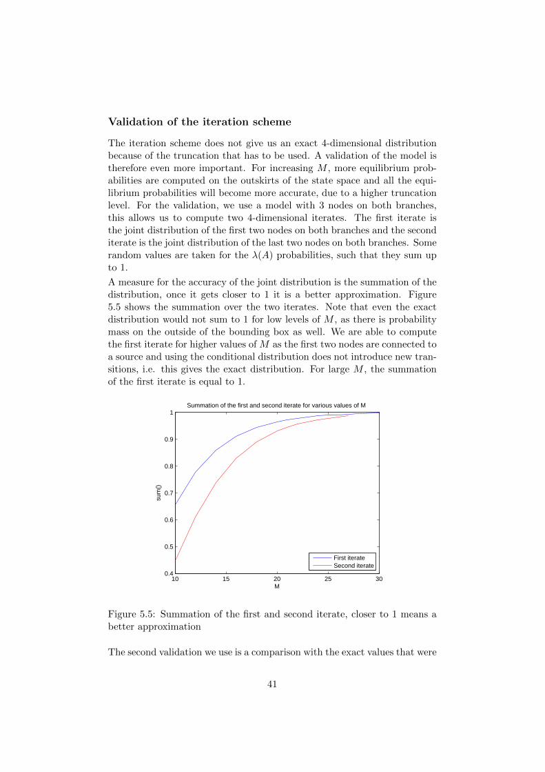
The iteration scheme does not give us an exact 4-dimensional distributionbecause of the truncation that has to be used. A validation of the model istherefore even more important. For increasing M , more equilibrium prob-abilities are computed on the outskirts of the state space and all the equi-librium probabilities will become more accurate, due to a higher truncationlevel. For the validation, we use a model with 3 nodes on both branches,this allows us to compute two 4-dimensional iterates. The first iterate isthe joint distribution of the first two nodes on both branches and the seconditerate is the joint distribution of the last two nodes on both branches. Somerandom values are taken for the λ(A) probabilities, such that they sum upto 1.
A measure for the accuracy of the joint distribution is the summation of thedistribution, once it gets closer to 1 it is a better approximation. Figure5.5 shows the summation over the two iterates. Note that even the exactdistribution would not sum to 1 for low levels of M , as there is probabilitymass on the outside of the bounding box as well. We are able to computethe first iterate for higher values of M as the first two nodes are connected toa source and using the conditional distribution does not introduce new tran-sitions, i.e. this gives the exact distribution. For large M , the summationof the first iterate is equal to 1.
10 15 20 25 300.4
0.5
0.6
0.7
0.8
0.9
1
M
sum
()
Summation of the first and second iterate for various values of M
First iterateSecond iterate
Figure 5.5: Summation of the first and second iterate, closer to 1 means abetter approximation
The second validation we use is a comparison with the exact values that were
41
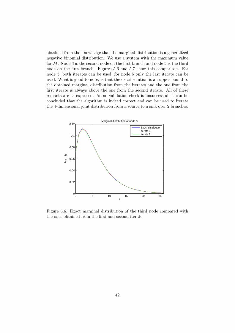
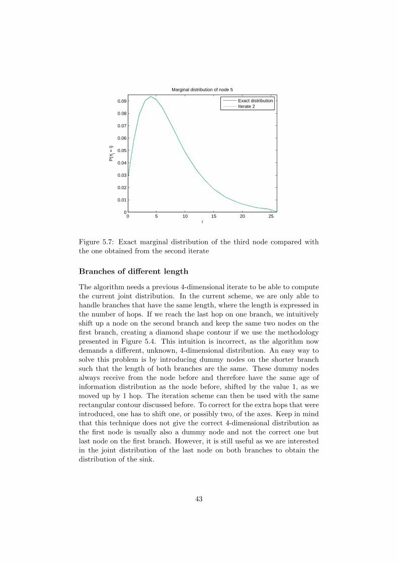
obtained from the knowledge that the marginal distribution is a generalizednegative binomial distribution. We use a system with the maximum valuefor M . Node 3 is the second node on the first branch and node 5 is the thirdnode on the first branch. Figures 5.6 and 5.7 show this comparison. Fornode 3, both iterates can be used, for node 5 only the last iterate can beused. What is good to note, is that the exact solution is an upper bound tothe obtained marginal distribution from the iterates and the one from thefirst iterate is always above the one from the second iterate. All of theseremarks are as expected. As no validation check is unsuccessful, it can beconcluded that the algorithm is indeed correct and can be used to iteratethe 4-dimensional joint distribution from a source to a sink over 2 branches.
0 5 10 15 20 250
0.02
0.04
0.06
0.08
0.1
0.12
i
P(π
i = i)
Marginal distribution of node 3
Exact distributionIterate 1Iterate 2
Figure 5.6: Exact marginal distribution of the third node compared withthe ones obtained from the first and second iterate
42
0 5 10 15 20 250
0.01
0.02
0.03
0.04
0.05
0.06
0.07
0.08
0.09
i
P(π
i = i)
Marginal distribution of node 5
Exact distributionIterate 2
Figure 5.7: Exact marginal distribution of the third node compared withthe one obtained from the second iterate
Branches of different length
The algorithm needs a previous 4-dimensional iterate to be able to computethe current joint distribution. In the current scheme, we are only able tohandle branches that have the same length, where the length is expressed inthe number of hops. If we reach the last hop on one branch, we intuitivelyshift up a node on the second branch and keep the same two nodes on thefirst branch, creating a diamond shape contour if we use the methodologypresented in Figure 5.4. This intuition is incorrect, as the algorithm nowdemands a different, unknown, 4-dimensional distribution. An easy way tosolve this problem is by introducing dummy nodes on the shorter branchsuch that the length of both branches are the same. These dummy nodesalways receive from the node before and therefore have the same age ofinformation distribution as the node before, shifted by the value 1, as wemoved up by 1 hop. The iteration scheme can then be used with the samerectangular contour discussed before. To correct for the extra hops that wereintroduced, one has to shift one, or possibly two, of the axes. Keep in mindthat this technique does not give the correct 4-dimensional distribution asthe first node is usually also a dummy node and not the correct one butlast node on the first branch. However, it is still useful as we are interestedin the joint distribution of the last node on both branches to obtain thedistribution of the sink.
43
Chapter summary
This chapter discussed a network consisting of two paths leading from sourceto the sink. We were interested in the marginal distribution of the sink.An algorithm was derived and validated to iteratively compute joint dis-tributions of four dimensions, such that the number of operations is linearin the number joint distributions. Problems concerning memory and timewere tackled by gaining insight into Matlab routines and memory manage-ment. We have validated the iteration scheme and the obtained results areas expected. Finally, it was shown that the algorithm is able to derive themarginal distribution for branches of different length.
44
Chapter 6
Conclusion
In this report we have introduced an abstract model of situation awarenessnetworks and have specifically limited us to Bernoulli channel and receptionpolicies. Even though this is a simplification of policies used in practice,the performance analysis done still gives great insights into possible solvingmethods. Using this model, the age of information was studied in greatdetail.
We have distinguished between two types of models. The first type are thesingle hop networks, consisting of sets of two nodes. By using the knowledgeobtained from small numbers of single hops, an algorithm was derived thatcan compute the joint distribution of an arbitrary number of single hops.The second type is the line of relays. By studying this network, it was foundthat the marginal distribution of a node in a tree-structured network is ageneralized negative binomial. An algorithm capable of finding joint distri-butions of sets of succeeding nodes in these lines of relays was introducedand validated as well.
Finally, a network consisting of two branches from source to sink was studied.We have succeeding in deriving an algorithm that computes joint distribu-tions of four dimensions, such that the number of operations is linear in thenumber of joint distributions. Each iterate we move one hop closer (on eachbranch) to the sink. Problems concerning memory and time were tackled bygaining insight into Matlab routines and memory management. The algo-rithm is also capable of handling branches of different length by introducingdummy links, without changing the joint distribution of the last two nodes,needed for the marginal distribution of the sink. This iteration scheme wasvalidated with the help of the generalized negative binomial expressions andthe already validated algorithms of the single hop networks and the line ofrelays.
A first step has been set in the field of analysis of age of information insituation awareness networks. For future work, one should improve the
45
algorithm to be able to deal with an arbitrary number of paths from sourceto sink. Ultimately, a scheme should be used that can obtain mean ages ofinformation and marginal distribution for every layout of the network. Ifone succeeds herein, the next thing to do is tackle real-time control problemsconcerning the transmission probabilities q where the age of informationis minimized. Another option would be to study different, more complexpolicies or even moving nodes such as in road traffic situation awarenessnetworks. The analysis could be coupled with more extensive simulationsto give evidence for the algorithms.
46

Bibliography
[1] Augustin Chaintreau, Jean-Yves Le Boudec, Nikodin Ristanovic TheAge of Gossip: Spatial Mean Field Regime. SIGMETRICS ’09, 2009, pp.109-120.
[2] Xiuli Chao A queueing network model with catastrophes and product formsolution. Operations Research Letters 18, 1995, pp. 75-79.
[3] Gideon Weiss Stochastic bounds on distributions of optimal value func-tions with applications to pert, network flows and reliability. Annals ofOperations Research 1, 1984, pp. 59-65.
[4] Pierpaolo Pontrandolfo Project duration in stochastic networks by thePERT-path technique. International Journal of Project Management 18,2000, pp. 215-222.
[5] Arunava Banerjee, Anand Paul On path correlation and PERT bias.European Journal of Operational Research 189, 2008, pp. 1208-1216
[6] Pascal Getreuer Writing fast MATLAB code. MathWorks, 2009
47
Appendix A
Derivation of the covariancefor a network with two singlehops
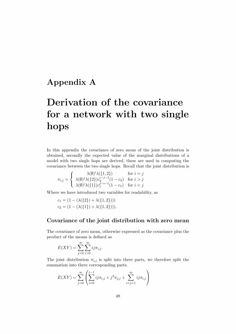
In this appendix the covariance of zero mean of the joint distribution isobtained, secondly the expected value of the marginal distributions of amodel with two single hops are derived, these are used in computing thecovariance between the two single hops. Recall that the joint distribution is
πi,j =
λ(∅)iλ({1, 2}) for i = j
λ(∅)jλ({2})ci−j−12 (1− c2) for i > j
λ(∅)iλ({1})cj−i−11 (1− c1) for i < j
Where we have introduced two variables for readability, as
c1 = (1− (λ({2}) + λ({1, 2})))c2 = (1− (λ({1}) + λ({1, 2}))).
Covariance of the joint distribution with zero mean
The covariance of zero mean, otherwise expressed as the covariance plus theproduct of the means is defined as
E(XY ) =∞∑j=0
∞∑i=0
ijπi,j .
The joint distribution πi,j is split into three parts, we therefore split thesummation into three corresponding parts.
E(XY ) =
∞∑j=0
j−1∑i=0
ijπi,j + j2πj,j +
∞∑i=j+1
ijπi,j
48
For clarity, we solve the summations part by part.
∞∑j=0
j−1∑i=0
ijπi,j =∞∑y=0
y−1∑i=0
ijλ({1})(1− c1)
c1λ(∅)i c
j1
ci1
=λ({1})(1− c1)
c1
∞∑j=0
jcj1
j−1∑i=0
i
(λ(∅)c1
)i=λ({1})(1− c1)c1(
λ(∅)c1− 1)2
∞∑j=0
jcj1
(j
(λ(∅)c1
)j(λ(∅)c1− 1)
−(λ(∅)c1
)j λ(∅)c1
+λ(∅)c1
)=λ({1})(1− c1)c1(
λ(∅)c1− 1)2
(−λ(∅)(λ(∅) + 1)(λ(∅)c1
− 1)
(λ(∅)− 1)3
− λ(∅)2
c1(λ(∅)− 1)2+
λ(∅)(c1 − 1)2
)If we use
∞∑j=0
∞∑i=j+1
ijπi,j =
∞∑i=0
i−1∑j=0
ijπi,j
and the above result for the first part of the summation, we can analogouslyderive the expression for the last part of the summation, where i > j.
∞∑j=0
∞∑i=j+1
ijπi,j =λ({2})(1− c2)c2(
λ(∅)c2− 1)2
(−λ(∅)(λ(∅) + 1)(λ(∅)c2
− 1)
(λ(∅)− 1)3
− λ(∅)2
c2(λ(∅)− 1)2+
λ(∅)(c2 − 1)2
)The simpler term of the summation is the second term, where i = j, whichcan be expressed as
∞∑j=0
j2πj,j =
∞∑j=0
λ({1, 2})j2λ(∅)j = λ({1, 2})−λ(∅)(λ(∅) + 1)
(λ(∅)− 1)3.
49
The summation of these three terms is equal to E(XY ).
E(XY ) =λ({1})(1− c1)c1(
λ(∅)c1− 1)2
(−λ(∅)(λ(∅) + 1)(λ(∅)c1
− 1)
(λ(∅)− 1)3− λ(∅)2
c1(λ(∅)− 1)2
+λ(∅)
(c1 − 1)2
)+ λ({1, 2})−λ(∅)(λ(∅) + 1)
(λ(∅)− 1)3
+λ({2})(1− c2)c2(
λ(∅)c2− 1)2
(−λ(∅)(λ(∅) + 1)(λ(∅)c2
− 1)
(λ(∅)− 1)3− λ(∅)2
c2(λ(∅)− 1)2
+λ(∅)
(c2 − 1)2
)
Expected value of the marginal distributions
Recall that the marginal distributions were given as
π(X)i = (1− (λ({1}) + λ({1, 2})))i(λ({1}) + λ({1, 2})) = (1− c2)ci2π(Y )j = (1− (λ({2}) + λ({1, 2})))j(λ({2}) + λ({1, 2})) = (1− c1)cj1.
The expected value of the two discrete marginal distributions are obtainedas follows
E(X) =
∞∑i=0
iπ(X)i = (1− c2)
∞∑i=0
ici2 =c2
1− c2
E(Y ) =
∞∑j=0
jπ(Y )j = (1− c1)
∞∑j=0
jcj1 =c1
1− c1.
Covariance
A measure of interference of two random variables X and Y is the covariance.Covariance is defined as
Cov(X,Y ) = E((X − E(X))(Y − E(Y )))
= E(XY −XE(Y )− Y E(X) + E(X)E(Y ))
= E(XY )− E(X)E(Y ).
50
If we now use the expected value of the joint distribution and the marginaldistribution, we get
Cov(X,Y ) =λ({1})(1− c1)c1(
λ(∅)c1− 1)2
(−λ(∅)(λ(∅) + 1)(λ(∅)c1
− 1)
(λ(∅)− 1)3− λ(∅)2
c1(λ(∅)− 1)2
+λ(∅)
(c1 − 1)2
)+ λ({1, 2})−λ(∅)(λ(∅) + 1)
(λ(∅)− 1)3
+λ({2})(1− c2)c2(
λ(∅)c2− 1)2
(−λ(∅)(λ(∅) + 1)(λ(∅)c2
− 1)
(λ(∅)− 1)3− λ(∅)2
c2(λ(∅)− 1)2
+λ(∅)
(c2 − 1)2
)− c2
1− c2c1
1− c1.
Using the symbolic toolbox in Matlab, we can simplify this expression to
Cov(X,Y ) =λ(∅)λ({1, 2})− λ({1})λ({2})
(λ({1}) + λ({1, 2}))(λ({2}) + λ({1, 2}))(1− λ(∅))
51
Appendix B
M-file: Function forcomputing λj(B)
This M-file computes the probability of successful reception for networksthat have at most one coupled node. Note that some lines were broken off,such that they fit on the page.
1 function [ lambdaSet lambdaProb ] = lambdaLinks(link,coupled,2 nodeTransProb,K)3 %%%%%%%%%%%%%%%%%%%%%%%%%%%%%%%%%%%%%%%%%%%%%%%%%%%%%%%%%%%%%%%%%%%%%%%%%%4 % Computes lambda for links, the input arguments are5 % o link = [ ID From To Prob ], the last two should always be dummy6 % links with p = 1 and their correct q.7 % o coupled are sets of nodes (supplied as a cell) that are connected to8 % the same transmitting node.9 % o nodeTransProb is the probability 'q' of transmission for all nodes,
10 % note that we include the source, node 0, as the first element of11 % this vector and therefore all indices are shifted by 1.12 % o K is a cell with neighbouring nodes for all nodes13 %%%%%%%%%%%%%%%%%%%%%%%%%%%%%%%%%%%%%%%%%%%%%%%%%%%%%%%%%%%%%%%%%%%%%%%%%%14
15 Nlink = link(:,1);16 linkFrom = link(:,2); linkTo = link(:,3); linkProb = link(:,4);17
18 lambdaSet = nchoose(Nlink);19 lambdaProb = zeros(numel(lambdaSet),1);20
21 for i = 1:numel(lambdaSet)22
23 B = lambdaSet{i};24
25 clear DSet DSubSet26
27 DSubSet = nchoose(setxor(Nlink,B)); DSubSet(end+1) = {[]}; %#ok<AGROW>28
52
29 DSet = cell(numel(DSubSet),1);30 for ii = 1:numel(DSubSet)31 DSet(ii,:) = {[ B DSubSet{ii} ]};32 end33
34 for iii = 1:numel(coupled)35 DSet = cellfun(@(c)addTx(c,coupled{iii}),DSet,36 'UniformOutput',false);37 end38
39 DSet = uniqueCellArray(DSet);40
41 for j = 1:numel(DSet)42 D = DSet{j};43
44 setTx = unique(linkFrom(D));45 setNoTx = setxor(linkFrom,setTx);46 setRx = B;47 tmpSet = [];48 for jj = 1:numel(setTx)49 tmpSet = [ tmpSet find(linkFrom == setTx(jj))' ]; %#ok<AGROW>50 end51 setNoRx = setxor(setRx,tmpSet);52
53 tmp = 1;54 for k = 1:length(setNoTx)55 tmp = tmp*(1−nodeTransProb(setNoTx(k)+1));56 end57 for k = 1:length(setTx)58 tmp = tmp*nodeTransProb(setTx(k)+1);59 end60 for k = 1:length(setRx)61 tmp = tmp*rInt(setRx(k));62 end63 for k = 1:length(setNoRx)64 tmp = tmp*(1−rInt(setNoRx(k)));65 end66
67 lambdaProb(i) = lambdaProb(i) + tmp;68
69 end70
71 end72
73 lambdaProb(end+1) = 1 − sum(lambdaProb);74 lambdaSet(end+1) = {[]};75
76 [ lambdaSet lambdaProb ] = lambdaSmallerNetwork(lambdaSet,77 lambdaProb,Nlink(1:(end−1)),Nlink);78
79 function pInt = rInt(j)80
81 if ismember(linkTo(j),linkFrom(D))82 pInt = 0;
53
83 else84 L = intFact;85 pInt = L*linkProb(j);86 end87
88 function L = intFact89 L = 1/(numel(intersect(D,K{linkTo(j)}))+1);90 end91
92 end93
94 end
54
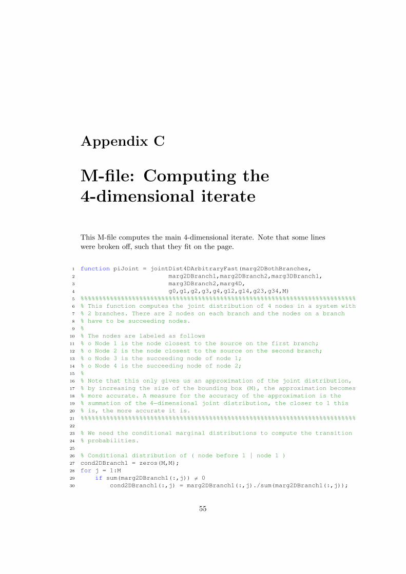
Appendix C
M-file: Computing the4-dimensional iterate
This M-file computes the main 4-dimensional iterate. Note that some lineswere broken off, such that they fit on the page.
1 function piJoint = jointDist4DArbitraryFast(marg2DBothBranches,2 marg2DBranch1,marg2DBranch2,marg3DBranch1,3 marg3DBranch2,marg4D,4 g0,g1,g2,g3,g4,g12,g14,g23,g34,M)5 %%%%%%%%%%%%%%%%%%%%%%%%%%%%%%%%%%%%%%%%%%%%%%%%%%%%%%%%%%%%%%%%%%%%%%%%%%%6 % This function computes the joint distribution of 4 nodes in a system with7 % 2 branches. There are 2 nodes on each branch and the nodes on a branch8 % have to be succeeding nodes.9 %
10 % The nodes are labeled as follows11 % o Node 1 is the node closest to the source on the first branch;12 % o Node 2 is the node closest to the source on the second branch;13 % o Node 3 is the succeeding node of node 1;14 % o Node 4 is the succeeding node of node 2;15 %16 % Note that this only gives us an approximation of the joint distribution,17 % by increasing the size of the bounding box (M), the approximation becomes18 % more accurate. A measure for the accuracy of the approximation is the19 % summation of the 4−dimensional joint distribution, the closer to 1 this20 % is, the more accurate it is.21 %%%%%%%%%%%%%%%%%%%%%%%%%%%%%%%%%%%%%%%%%%%%%%%%%%%%%%%%%%%%%%%%%%%%%%%%%%%22
23 % We need the conditional marginal distributions to compute the transition24 % probabilities.25
26 % Conditional distribution of ( node before 1 | node 1 )27 cond2DBranch1 = zeros(M,M);28 for j = 1:M29 if sum(marg2DBranch1(:,j)) 6= 030 cond2DBranch1(:,j) = marg2DBranch1(:,j)./sum(marg2DBranch1(:,j));
55
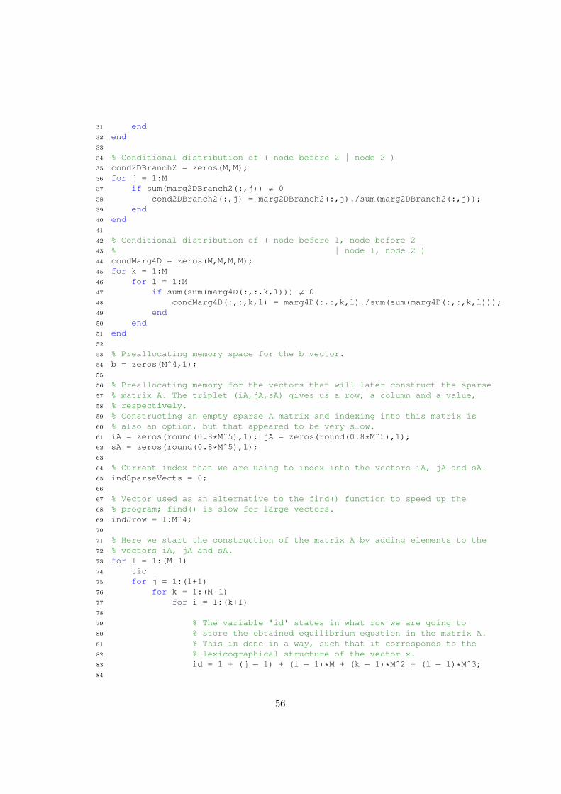
31 end32 end33
34 % Conditional distribution of ( node before 2 | node 2 )35 cond2DBranch2 = zeros(M,M);36 for j = 1:M37 if sum(marg2DBranch2(:,j)) 6= 038 cond2DBranch2(:,j) = marg2DBranch2(:,j)./sum(marg2DBranch2(:,j));39 end40 end41
42 % Conditional distribution of ( node before 1, node before 243 % | node 1, node 2 )44 condMarg4D = zeros(M,M,M,M);45 for k = 1:M46 for l = 1:M47 if sum(sum(marg4D(:,:,k,l))) 6= 048 condMarg4D(:,:,k,l) = marg4D(:,:,k,l)./sum(sum(marg4D(:,:,k,l)));49 end50 end51 end52
53 % Preallocating memory space for the b vector.54 b = zeros(Mˆ4,1);55
56 % Preallocating memory for the vectors that will later construct the sparse57 % matrix A. The triplet (iA,jA,sA) gives us a row, a column and a value,58 % respectively.59 % Constructing an empty sparse A matrix and indexing into this matrix is60 % also an option, but that appeared to be very slow.61 iA = zeros(round(0.8*Mˆ5),1); jA = zeros(round(0.8*Mˆ5),1);62 sA = zeros(round(0.8*Mˆ5),1);63
64 % Current index that we are using to index into the vectors iA, jA and sA.65 indSparseVects = 0;66
67 % Vector used as an alternative to the find() function to speed up the68 % program; find() is slow for large vectors.69 indJrow = 1:Mˆ4;70
71 % Here we start the construction of the matrix A by adding elements to the72 % vectors iA, jA and sA.73 for l = 1:(M−1)74 tic75 for j = 1:(l+1)76 for k = 1:(M−1)77 for i = 1:(k+1)78
79 % The variable 'id' states in what row we are going to80 % store the obtained equilibrium equation in the matrix A.81 % This in done in a way, such that it corresponds to the82 % lexicographical structure of the vector x.83 id = 1 + (j − 1) + (i − 1)*M + (k − 1)*Mˆ2 + (l − 1)*Mˆ3;84
56
85 % The state space is split into 25 different regions, each86 % region has its own incoming transitions. We call a87 % nested subfunction tr4D (transition probabilities in88 % 4 dimensions) to compute a J matrix and an entry in the b89 % vector.90 % The J matrix is M−by−M−by−M−by−M, it contains the91 % coefficients of the equilibrium equation in matrix form.92 if isequal([ i j k l ],[ 2 2 1 1 ]) % 793 [ J b(id) ] = tr4D([ 0 0 0 1 0 0 0 0 0 ]);94 elseif isequal([ i j k ],[ 2 1 1 ]) && l ≥ 2 % 895 [ J b(id) ] = tr4D([ 0 0 1 0 0 0 0 0 0 ]);96 elseif isequal([ i k ],[ 2 1 ]) && j == (l+1) && j ≥
3 % 997 [ J b(id) ] = tr4D([ 0 0 1 1 0 0 1 0 0 ]);98 elseif isequal([ i k ],[ 2 1 ]) && l ≥ j && j ≥ 2 % 1099 [ J b(id) ] = tr4D([ 0 0 1 0 0 0 1 0 0 ]);
100 elseif isequal([ i j l ],[ 1 2 1 ]) && k ≥ 2 % 12101 [ J b(id) ] = tr4D([ 0 1 0 0 0 0 0 0 0 ]);102 elseif isequal([ i j ],[ 1 1 ]) && k ≥ 2 && l ≥ 2 % 13103 [ J b(id) ] = tr4D([ 1 0 0 0 0 0 0 0 0 ]);104 elseif i == 1 && k ≥ 2 && j == (l+1) && j ≥ 3 % 14105 [ J b(id) ] = tr4D([ 1 1 0 0 1 0 0 0 0 ]);106 elseif i == 1 && k ≥ 2 && l ≥ j && j ≥ 2 % 15107 [ J b(id) ] = tr4D([ 1 0 0 0 1 0 0 0 0 ]);108 elseif i == (k+1) && i ≥ 3 && isequal([ j l ],[ 2 1 ]) % 17109 [ J b(id) ] = tr4D([ 0 1 0 1 0 0 0 1 0 ]);110 elseif i == (k+1) && i ≥ 3 && j == 1 && l ≥ 2 % 18111 [ J b(id) ] = tr4D([ 1 0 1 0 0 1 0 0 0 ]);112 elseif i == (k+1) && i ≥ 3 && j == (l+1) && j ≥ 3 % 19113 [ J b(id) ] = tr4D([ 1 1 1 1 1 1 1 1 1 ]);114 elseif i == (k+1) && i ≥ 3 && l ≥ j && j ≥ 2 % 20115 [ J b(id) ] = tr4D([ 1 0 1 0 1 1 1 0 1 ]);116 elseif k ≥ i && i ≥ 2 && isequal([ j l ],[ 2 1 ]) % 22117 [ J b(id) ] = tr4D([ 0 1 0 0 0 0 0 1 0 ]);118 elseif k ≥ i && i ≥ 2 && j == 1 && l ≥ 2 % 23119 [ J b(id) ] = tr4D([ 1 0 0 0 0 1 0 0 0 ]);120 elseif k ≥ i && i ≥ 2 && j == (l+1) && j ≥ 3 % 24121 [ J b(id) ] = tr4D([ 1 1 0 0 1 1 0 1 1 ]);122 elseif k ≥ i && i ≥ 2 && l ≥ j && j ≥ 2 % 25123 [ J b(id) ] = tr4D([ 1 0 0 0 1 1 0 0 1 ]);124 else125 [ J b(id) ] = tr4D([ 0 0 0 0 0 0 0 0 0 ]);126 end127
128 % The matrix J has to rearranged into a row and the129 % non−zero elements (J only contains non−negative values)130 % are stored in sA, the location of the element is stored131 % in iA (row) and jA (column).132 Jrow = J(:);133 JrowPos = indJrow(Jrow > 0);134 JrowPosNum = numel(JrowPos);135
136 iA( (indSparseVects+1):(indSparseVects+JrowPosNum) ) =137 id*ones(1,JrowPosNum);
57
138 jA( (indSparseVects+1):(indSparseVects+JrowPosNum) ) =139 JrowPos;140 sA( (indSparseVects+1):(indSparseVects+JrowPosNum) ) =141 Jrow(JrowPos);142
143 % We update the index used to store the positive values of144 % J in iA, jA and sA.145 indSparseVects = indSparseVects + JrowPosNum;146
147 end148 end149 end150
151 % Iteration progress and memory usage is printed to the command window152 display(sprintf('Iteration %d out of %d \t−−\t %0.5g seconds\n'153 'Storage used \t %0.5g, \t out of \t %0.5g\n'154 ,l,M−1,toc,nnz(iA),length(iA)))155
156 end157
158 % Clear all temporary files, such that we have more memory available for159 % the matrix A to be added to the memory.160 clear Jrow JrowPos JrowPosNum indSparseVects J161 clear condMarg4D cond2DBranch1 cond2DBranch2162
163 % Construct the matrix A by using the indices iA and jA and the164 % corresponding values sA. We subtract the value 1 from each row, as we165 % want all variables x on one side.166 % (The system is actually Ax − b = x, which leads to (A−I)x = b )167 A = sparse(iA(1:nnz(iA)),jA(1:nnz(jA)),sA(1:nnz(sA)),Mˆ4,Mˆ4);168 A = A − spdiags(ones(Mˆ4,1),0,Mˆ4,Mˆ4);169
170 % Solve the system171 x = A\b;172
173 % Reconstruct the 4−dimensional joint distribution by obtaining the i, j, k174 % and l value from the row number.175 piJoint = zeros(M,M,M,M);176 for n = 1:Mˆ4177 l = ceil(n/Mˆ3);178 k = ceil( (n − (l−1)*Mˆ3) / Mˆ2 );179 i = ceil( (n − (l−1)*Mˆ3 − (k−1)*Mˆ2 ) / M );180 j = n − (l−1)*Mˆ3 − (k−1)*Mˆ2 − (i−1)*M;181 piJoint(i,j,k,l) = x(n);182 end183
184 %% Nested function to compute the transition probabilities185
186 function [ J, b ] = tr4D(r)187 % The variable r is a list describing type of incoming transitions188 % [ lambda(1,2) lambda(1,4) lambda(2,3) lambda(3,4) ...189 % lambda(1) lambda(2) lambda(3) lambda(4) lambda(\emptyset) ]190
191 % Preallocating memory for J and b.
58
192 J = zeros(M,M,M,M);193 b = 0;194
195 % Indices used for the conditional distribution, this has to be used196 % due to the structure of the equilibrium equations.197 iB = max(i−1,1):k; jB = max(j−1,1):l;198
199 % We check for all possible incoming transitions and compute the ones200 % that are needed for that region.201 if r(1)202 J(jB,iB,k−1,l−1) = J(jB,iB,k−1,l−1) + ...203 g12*reshape(condMarg4D(i,j,iB,jB),numel(iB),numel(jB))';204 end205 if r(2)206 b = b − g14 * cond2DBranch1(i,iB) * marg3DBranch1(iB,j−1,k−1);207 end208 if r(3)209 b = b − g23 * cond2DBranch2(j,jB) * marg3DBranch2(i−1,jB,l−1)';210 end211 if r(4)212 b = b − g34 * marg2DBothBranches(i−1,j−1);213 end214 if r(5)215 J(j−1,iB,k−1,l−1) = J(j−1,iB,k−1,l−1) + g1 * cond2DBranch1(i,iB);216 end217 if r(6)218 J(jB,i−1,k−1,l−1) = J(jB,i−1,k−1,l−1) + g2 * cond2DBranch2(j,jB)';219 end220 if r(7)221 b = b − g3 * marg3DBranch2(i−1,j−1,l−1);222 end223 if r(8)224 b = b − g4 * marg3DBranch1(i−1,j−1,k−1);225 end226 if r(9)227 J(j−1,i−1,k−1,l−1) = J(j−1,i−1,k−1,l−1) + g0;228 end229
230 end231
232 end
59

Appendix D
M-file: Using the iterationscheme
This M-file is used to run the iteration scheme, it calls all the necessaryfunctions. In the current state, it runs the example shown in the proof ofconcept section. Note that some lines were broken off, such that they fit onthe page.
1 %% Iteration run file2 %3 % We look at a model consisting of 2 branches, both connected to the same4 % source.5 % o The node closest to the source on the first branch is node 1;6 % o The node closest to the source on the second branch is node 2;7 % o The succeeding node on the first branch is node 3;8 % o The succeeding node on the second branch is node 4.9 %
10 % This file iteratively computes a 4−dimensional joint distribution of two11 % succeeding nodes on the first branch and two succeeding nodes on the12 % second branch.13
14 clc, clear all15
16 %% System parameters17
18 % Homogenous system19 p = 0.9;20 q = 0.5;21
22 % Specifying the links [ ID from to prob ]23 link = [ 1 0 1 p ;24 2 0 2 p ;25 3 1 3 p ;26 4 2 4 p ;27 5 3 5 p ;
60
28 6 4 6 p ;29 7 5 7 p ;30 8 6 8 p ;31 9 7 9 p ;32 10 8 9 p ;33 11 9 10 1 ]; % dummy link34
35 Nmax = link(end,1); N = 1:(Nmax − 1);36
37 Nhops = 4;38
39 % The two links that are coupled at the source40 coupled = { [ 1 2 ] };41
42 % Probability of transmission for each node43 nodeTransProb = ones(Nmax+1,1)*q;44
45 % Neighbouring nodes that affect successful reception probabilities46 K = cell(Nmax,1);47
48 [ lambdaSet lambdaProb ] = lambdaLinks(link,coupled,nodeTransProb,K);49
50 %% Iteration parameters51
52 % Size of the bounding box53 M = 20;54
55 %% Creating the input for the iteration scheme56
57 % Reception probabilities for the first four nodess of the system58 [ lambdaSetCurr lambdaProbCurr ] = lambdaSmallerNetwork(lambdaSet,59 lambdaProb,[1 2 3 4],N);60
61 l0 = lambdaProbCurr(fI(lambdaSetCurr,[]));62 l1 = lambdaProbCurr(fI(lambdaSetCurr,[1]));63 l2 = lambdaProbCurr(fI(lambdaSetCurr,[2]));64 l3 = lambdaProbCurr(fI(lambdaSetCurr,[3]));65 l4 = lambdaProbCurr(fI(lambdaSetCurr,[4]));66 l12 = lambdaProbCurr(fI(lambdaSetCurr,[1 2]));67 l14 = lambdaProbCurr(fI(lambdaSetCurr,[1 4]));68 l23 = lambdaProbCurr(fI(lambdaSetCurr,[2 3]));69 l34 = lambdaProbCurr(fI(lambdaSetCurr,[3 4]));70
71 % Joint distribution of ( node 1, node 2)72 marg2DBothBranches = jointDistSameTx(l0+l3+l4+l34,l1+l14,l2+l23,l12,M);73
74 % Joint distribution of ( source, node 1 )75 marg2DBranch1 = zeros(M,M);76 marg2DBranch1(1,:) = sum(marg2DBothBranches,2);77
78 % Joint distribution of ( source, node 2 )79 marg2DBranch2 = zeros(M,M);80 marg2DBranch2(1,:) = sum(marg2DBothBranches,2);81
61
82 % Joint distribution of ( source, source, node 1, node 2 )83 marg4D = zeros(M,M,M,M);84 marg4D(1,1,:,:) = marg2DBothBranches;85
86 % Joint distribution of ( node 1, node 2, node 3 )87 marg3DBranch1 = jointDist3DArbitraryFast(marg2DBothBranches,88 marg2DBranch1,marg2DBranch2,marg4D,89 l0+l4,l1+l14,l2,l3+l34,l12,l23,M);90
91 % Joint distribution of ( node 1, node 2, node 4 )92 marg3DBranch2 = jointDist3DArbitraryFastAlt(marg2DBothBranches,93 marg2DBranch1,marg2DBranch2,marg4D,94 l0+l3,l1,l2+l23,l4+l34,l12,l14,M);95
96 %% First iterate97
98 display(sprintf('\n\t Iterate number: \t %g',1))99
100 % Joint disitrubtion of ( node 1, node 2, node 3, node 4 )101 marg4DIter = jointDist4DArbitraryFast(marg2DBothBranches,marg2DBranch1,102 marg2DBranch2,marg3DBranch1,marg3DBranch2,marg4D,103 l0,l1,l2,l3,l4,l12,l14,l23,l34,M);104
105 sum(sum(sum(sum(marg4DIter))))106
107 %% Obtaining the input for the next iterate108
109 for iter = 2:Nhops110
111 % Number of the links we are considering for this iterate112 n = [ 2*(iter−1)+1 2*(iter−1)+2 2*(iter−1)+3 2*(iter−1)+4 ];113
114 % Reception probabilities for the current iterate115 [ lambdaSetCurr lambdaProbCurr ] =116 lambdaSmallerNetwork(lambdaSet,lambdaProb,n,N);117
118 l0 = lambdaProbCurr(fI(lambdaSetCurr,[]));119 l1 = lambdaProbCurr(fI(lambdaSetCurr,[ n(1) ]));120 l2 = lambdaProbCurr(fI(lambdaSetCurr,[ n(2) ]));121 l3 = lambdaProbCurr(fI(lambdaSetCurr,[ n(3) ]));122 l4 = lambdaProbCurr(fI(lambdaSetCurr,[ n(4) ]));123 l12 = lambdaProbCurr(fI(lambdaSetCurr,[ n(1) n(2) ]));124 l14 = lambdaProbCurr(fI(lambdaSetCurr,[ n(1) n(4) ]));125 l23 = lambdaProbCurr(fI(lambdaSetCurr,[ n(2) n(3) ]));126 l34 = lambdaProbCurr(fI(lambdaSetCurr,[ n(3) n(4) ]));127
128 % Setting up for a new iterate129 marg4DIterPrev = marg4DIter;130
131 % 2−dimensional joint distributions132 marg2DBothBranches = squeeze(sum(sum(marg4DIterPrev,2),1));133 marg2DBranch1 = squeeze(sum(sum(marg4DIterPrev,4),2));134 marg2DBranch2 = squeeze(sum(sum(marg4DIterPrev,3),1));135
62
136 % 3−dimensional joint distributions137 marg3DBranch1 = jointDist3DArbitraryFast(marg2DBothBranches,138 marg2DBranch1,marg2DBranch2,marg4D,139 l0+l4,l1+l14,l2,l3+l34,l12,l23,M);140 marg3DBranch2 = jointDist3DArbitraryFastAlt(marg2DBothBranches,141 marg2DBranch1,marg2DBranch2,marg4D,142 l0+l3,l1,l2+l23,l4+l34,l12,l14,M);143
144 % New iterate145 display(sprintf('\n\t Iterate number: \t %g',iter))146 marg4DIter = jointDist4DArbitraryFast(marg2DBothBranches,147 marg2DBranch1,marg2DBranch2,marg3DBranch1,148 marg3DBranch2,marg4DIterPrev,149 l0,l1,l2,l3,l4,l12,l14,l23,l34,M);150
151 sum(sum(sum(sum(marg4DIter))))152 end
63