a fracture mechanics study of tungsten failure under high ... · lehrstuhl fur werkstoffkunde und...
TRANSCRIPT
Lehrstuhl fur Werkstoffkunde und Werkstoffmechanik mit
Materialprufamt fur den Maschinenbau
Technische Universitat Munchen
A Fracture Mechanics Study of Tungsten
Failure under High Heat Flux Loads
Muyuan Li
Vollstandiger Abdruck der von der Fakultat fur Maschinenwesen
der Technischen Universitat Munchen
zur Erlangung des akademischen Grades eines
Doktor-Ingenieurs (Dr.-Ing.)
genehmigten Dissertation.
Vorsitzender: Univ.-Prof. dr. ir. Daniel J. Rixen
Prufer der Dissertation:
1. Univ.-Prof. Dr. mont. habil. Dr. rer. nat. h. c. Ewald Werner
2. Univ.-Prof. Dr. rer. nat. Rudolf Neu
Die Dissertation wurde am 28.10.2014 bei der Technischen Universitat Munchen
eingereicht und durch die Fakultat fur Maschinenwesen
am 20.02.2015 angenommen.

iii
Announcement
Parts of the results presented in this dissertation have been published in the following articles:
Muyuan Li, Ewald Werner, Jeong-Ha You, Fracture mechanicalanalysis of tungsten armor failure
of a water-cooled divertor target, Fusion Engineering Design, 89 (2014) 2716-2725.
Muyuan Li, Mathias Sommerer, Ewald Werner, Stefan Lampenscherf, Thorsten Steinkopff, Philipp
Wolfrum, Jeong-Ha You, Experimental and computational study of damage behavior of tungsten
under high energy electron beam irradiation, Engineering Fracture Mechanics, 135 (2015) 64-80.
Muyuan Li, Ewald Werner, Jeong-Ha You, Cracking behavior of tungsten armor under ELM-like
thermal shock loads: A computational study, Nuclear Materials and Energy, 2 (2015) 1-11.
Muyuan Li, Ewald Werner, Jeong-Ha You, Influence of heat flux loading patterns on the surface
cracking features of tungsten armor under ELM-like thermalshocks, Journal of Nuclear Materials,
457 (2015) 256-265.

v
Abstract
The performance of fusion devices is highly dependent on plasma-facing components, which have
to withstand stationary thermal loads as well as the thermaltransients induced by the instabilities
of the plasma confinement. Tungsten is the most promising candidate material for armors in the
plasma-facing components in ITER and DEMO. However, the brittleness of tungsten below the
ductile-to-brittle transition temperature is very critical to the reliability of the plasma-facing compo-
nents. In this work, thermo-mechanical and fracture behaviors of tungsten are predicted numerically
under fusion relevant thermal loadings, which are short transient thermal loads induced by edge lo-
calized mode (ELM), slow high-energy-deposition thermal loads (e.g. Vertical Displacement Event
(VDE)) and stationary heat flux loads. The results are compared with the corresponding experi-
mental observations, and the good agreement between the experimental observations and numerical
predictions proves the validity of the computational approaches.
Zusammenfassung
Die Leistungsfahigkeit von Kernfusionsanlagen hangt stark von den dem Plasma zugewandten Kom-
ponenten ab, welche den stationaren thermischen Belastungen ebenso standhalten mussen wie ther-
mischen Belastungen, die auf Instabilitaten des Plasmas zuruckzufuhren sind. Fur ITER und DEMO
ist Wolfram als das vielversprechendste Material zum Schutz der plasmabelasteten Komponenten
anzusehen. Allerdings stellt die Sprodigkeit von Wolfram unterhalb der Sprod-Duktil-Ubergang-
stemperatur einen kritischen Faktor fur die Zuverlassigkeit dieser plasmabelasteten Komponenten
dar. Diese Arbeit zielt auf eine Prognose des thermo-mechanisches Verhaltens sowie des Bruchver-
haltens von Wolfram ab - basierend auf numerischen Ansatzen unter Berucksichtigung der fusions-
relevanten thermischen Belastungen aufgrund von kurzen transienten thermischen Belastungen im
Edge Localized Mode (ELM), einer langsamen hohen Energiedeposition unter thermischen Belas-
tungen (z.B. eine schnelle vertikale Verschiebung des Plasmas / Vertical Displacement Event (VDE))
sowie des stationaren Warmeflusses. Die numerischen Vorhersagen werden entsprechenden experi-
mentellen Beobachtungen gegenubergestellt - wobei eine guteUbereinstimmung die Gultigkeit der
zugrundeliegenden Berechnungsansatze dieser Arbeit unterstreicht.


vii
Acknowledgments
This dissertation has been carried out at the Institute of Materials Science and Mechanics of Materi-
als at the Technische Universitat Munchen with Siemens AG and Max Planck Institute as cooperation
partners.
First of all I would like to thank Prof. Ewald Werner for his guidance and for providing the op-
portunity to work on this topic. Furthermore, I would like tothank Prof. Rudolf Neu (Max Planck
Institute) for reviewing the work. I would like to thank Prof. Rixen for being the chairman for the
final defense.
I am very grateful to Prof. Jeong Ha You (Max Planck Institute) for giving me scientific supervision
and for leading me to the fusion science research community.
I deeply appreciate that Prof. Hubertus von Dewitz (SiemensAG), Dr. Stefan Lampenscherf
(Siemens AG) and Dr. Michael Metzger (Siemens AG) initiatedthis joint project and gave me
support and inspiration. Furthermore, I would like to thankDr. Philipp Wolfrum (Siemens AG) and
Dr. Thorsten Steinkopff (Siemens AG) for their support and our discussions.
I would like to give many thanks to M.Sc. Mathias Sommerer forproviding the experimental data
and for many fruitful discussions and his valuable advice.
I acknowledge Dr. Christian Krempaszky for his helpful advice and our discussions. I would like
to give special thanks to Yvonne Jahn for her support and organizational matters and Jinming Lu
for his tips on writing the manuscript. I would also like to extend my thanks to colleagues at the
Institute of Materials Science and Mechanics of Materials and Siemens AG, who have contributed
to this work and provided a lot of help in the past four years.
This work was funded by Siemens AG. The financial support is gratefully acknowledged.
Last but not least, I would like to thank my wife Quanji, my sonDongxu and my parents, who gave
me precious and constant support as well as motivation.
Muyuan Li
Garching, March 2015

List of Figures ix
List of Figures
1.1 History and outlook of the world energy consumption [1].. . . . . . . . . . . . . . . 2
1.2 Average nuclear binding energy per nucleon as a functionof number of nucleons in
the atomic nucleus. . . . . . . . . . . . . . . . . . . . . . . . . . . . . . . . . . .. 3
1.3 Experimentally determined cross sections. . . . . . . . . . .. . . . . . . . . . . . . 4
1.4 The deuterium-tritium fusion. . . . . . . . . . . . . . . . . . . . . .. . . . . . . . . 5
1.5 The tokamak principle. . . . . . . . . . . . . . . . . . . . . . . . . . . . .. . . . . 6
1.6 Artists impression of a fusion power plant [2]. . . . . . . . .. . . . . . . . . . . . . 7
1.7 ITER plasma-facing components [3]. . . . . . . . . . . . . . . . . .. . . . . . . . . 8
1.8 Plasma induced thermal loads on plasma facing components in ITER [4]. . . . . . . 9
1.9 Schematic of an ITER divertor cassette [3]. . . . . . . . . . . .. . . . . . . . . . . 10
1.10 ITER plasma-facing materials for the initial operation phase with hydrogen. . . . . . 11
1.11 Response of tungsten under electron beams. . . . . . . . . . . .. . . . . . . . . . . 12
2.1 Polar coordinates at the crack tip. . . . . . . . . . . . . . . . . . .. . . . . . . . . . 16
2.2 Illustration of three linearly independent cracking modes: mode I, opening; mode II,
sliding; mode III, tearing. . . . . . . . . . . . . . . . . . . . . . . . . . . .. . . . . 17
2.3 Illustration of the superposition principle used for the weight function method. . . . . 19
2.4 A prospective edge crack (dashed line) in a semi-infinitespace. . . . . . . . . . . . . 19
2.5 Schematic diagram for the domain integral concept. . . . .. . . . . . . . . . . . . . 21
2.6 The enriching strategy near the crack. . . . . . . . . . . . . . . .. . . . . . . . . . 24
2.7 Construction of initial level-set functions. . . . . . . . . .. . . . . . . . . . . . . . 25
2.8 The principle of the phantom node method. . . . . . . . . . . . . .. . . . . . . . . 26
2.9 Linear traction-separation response. . . . . . . . . . . . . . .. . . . . . . . . . . . 28
3.1 The magnetic geometry of a divertor tokamak and pressureprofiles of L- and H-
mode plasmas. . . . . . . . . . . . . . . . . . . . . . . . . . . . . . . . . . . . . . . 30
3.2 Electron beam test facility working principle [5]. . . . .. . . . . . . . . . . . . . . 32
3.3 Microstructures in a diagram of power density as a function of bulk temperature. . . 33
3.4 Crack near the edge of the loading area under a single pulseof 0.55 GW/m2 for 5 ms. 33
3.5 Thermal shock behavior of pure tungsten in two directions. . . . . . . . . . . . . . . 34
3.6 LM-images of the materials crack patterns under multiple thermal shocks. . . . . . . 34
x List of Figures
3.7 Crack patterns at cross-section of W-UHP and WTa5. . . . . . . .. . . . . . . . . . 35
3.8 Temperature predicted using analytical and numerical methods. . . . . . . . . . . . . 39
3.9 Temperature at the end of heating and the maximum temperature. . . . . . . . . . . 40
3.10 Maximum temperature as a function of depth. . . . . . . . . . .. . . . . . . . . . . 41
3.11 A schematic drawing of the simplified models. . . . . . . . . .. . . . . . . . . . . . 42
3.12 Meshes of axisymmetric model and a zoom-in. . . . . . . . . . .. . . . . . . . . . 43
3.13 Plastic strain in radial direction calculated by analytical and numerical methods. . . . 44
3.14 Stress in radial direction calculated by analytical and numerical methods. . . . . . . 44
3.15 A schematic drawing of stress-strain curves for different loadings. . . . . . . . . . . 45
3.16 Plastic strain in radial direction along the depth for different power densities. . . . . 46
3.17 Stress in radial direction along the depth for different power densities. . . . . . . . . 46
3.18 Plastic strain in radial direction for different base temperatures. . . . . . . . . . . . . 47
3.19 Stress in radial direction for different base temperatures. . . . . . . . . . . . . . . . 47
3.20 Fracture toughness as a function of temperature. . . . . .. . . . . . . . . . . . . . . 48
3.21 Stress intensity factors calculated for different loadings and base temperatures. . . . 49
3.22 The failure map. . . . . . . . . . . . . . . . . . . . . . . . . . . . . . . . . .. . . . 50
3.23 A schematic drawing and meshes of the model. . . . . . . . . . .. . . . . . . . . . 51
3.24 Temperature distribution at the end of heating. . . . . . .. . . . . . . . . . . . . . . 53
3.25 Surface temperature at various times. . . . . . . . . . . . . . .. . . . . . . . . . . . 54
3.26 Temperature at different depths at the end of heating. .. . . . . . . . . . . . . . . . 54
3.27 Distribution of plastic strain in radial direction at the end of heating. . . . . . . . . . 55
3.28 Distribution of plastic strain in radial direction at the end of cooling. . . . . . . . . . 56
3.29 Surface plastic strain in radial direction at various times. . . . . . . . . . . . . . . . 57
3.30 Plastic strain in radial direction at different depthsat the end of cooling. . . . . . . . 58
3.31 Distribution of stress in radial direction at the end ofheating. . . . . . . . . . . . . . 59
3.32 Distribution of stress in radial direction at the end ofcooling. . . . . . . . . . . . . . 59
3.33 Surface stress in radial direction at various times. . .. . . . . . . . . . . . . . . . . 60
3.34 Surface vertical displacement at the end of cooling fora power density of 1.27 GW/m2
and a base temperature of 20◦C. . . . . . . . . . . . . . . . . . . . . . . . . . . . . 60
3.35 Stress in radial direction at different depths at the end of cooling. . . . . . . . . . . . 61
3.36 Stress-mechanical strain in radial direction at different depths. . . . . . . . . . . . . 61
3.37 Surface temperature at the end of heating for differentpower densities. . . . . . . . . 62
3.38 Surface plastic strain for different power densities.. . . . . . . . . . . . . . . . . . . 62
3.39 Surface stress in radial direction for different powerdensities. . . . . . . . . . . . . . 63
3.40 Surface temperature at the end of heating for differentbase temperatures. . . . . . . 63
3.41 Surface plastic strain at the end of cooling for different base temperatures. . . . . . . 64
3.42 Equivalent plastic strain at the end of cooling for different base temperatures. . . . . 64
3.43 Surface stress in radial direction at the end of coolingfor different base temperatures. 65
List of Figures xi
3.44 Cracks predicted using XFEM with a global enriched feature. . . . . . . . . . . . . . 67
3.45 Enriched features defined in each small domain for XFEM simulations. . . . . . . . 68
3.46 Cracks predicted using XFEM for different power densities. . . . . . . . . . . . . . 69
3.47 Precrack for the calculation of theJ-integral. . . . . . . . . . . . . . . . . . . . . . 70
3.48 J-integral for a power density of 1.27 GW/m2. . . . . . . . . . . . . . . . . . . . . . 70
3.49 J-integral for different power densities and base temperatures. . . . . . . . . . . . . 72
3.50 Thermal shock behavior of tungsten samples. . . . . . . . . .. . . . . . . . . . . . 73
3.51 Considered spatial profiles at the top surface of the axisymmetric model. . . . . . . . 74
3.52 Different temporal scenarios considered. . . . . . . . . . .. . . . . . . . . . . . . . 75
3.53 Surface temperature at the end of heating of different HHF loading patterns. . . . . . 75
3.54 Surface plastic strain in radial direction at the end ofheating. . . . . . . . . . . . . . 76
3.55 Surface plastic strain in radial direction at the end ofcooling. . . . . . . . . . . . . . 77
3.56 Surface stress in radial direction at the end of cooling. . . . . . . . . . . . . . . . . . 77
3.57 Stress in radial direction at a depth of 0.2 mm at the end of cooling. . . . . . . . . . . 78
3.58 Cracks predicted without precrack for six HHF loading patterns. . . . . . . . . . . . 80
3.59 Crack predicted with a single precrack for three energy distributions. . . . . . . . . . 81
3.60 Cracks predicted using XFEM with two precracks assumed.. . . . . . . . . . . . . 82
3.61 Precrack definition for theJ-integral calculation. . . . . . . . . . . . . . . . . . . . 83
3.62 J-integral for the constant and the ramp uniform loadings. . .. . . . . . . . . . . . 83
3.63 J-integral for the constant and the ramp triangular loadingswith a steep slope. . . . . 84
3.64 J-integral for the constant and the ramp triangular loadingswith a gradual slope. . . 84
3.65 Direction of the maximum energy release rate for the constant uniform loading. . . . 85
3.66 Direction of the maximum energy release rate for the constant triangular loading
with a steep slope. . . . . . . . . . . . . . . . . . . . . . . . . . . . . . . . . . . .. 85
3.67 Direction of the maximum energy release rate for the constant triangular loading
with a gradual slope. . . . . . . . . . . . . . . . . . . . . . . . . . . . . . . . . .. 86
4.1 Schematic drawing of the cutting surface of the experimental facility. . . . . . . . . . 91
4.2 LSM and out-of-plane deformation images for 0.374 GW/m2. . . . . . . . . . . . . . 92
4.3 LSM and out-of-plane deformation images for 0.5 GW/m2. . . . . . . . . . . . . . . 92
4.4 LSM and out-of-plane deformation images for 0.624 GW/m2. . . . . . . . . . . . . . 92
4.5 FE mesh of the two-dimensional axisymmetric model. . . . .. . . . . . . . . . . . 94
4.6 Temperature distribution for a thermal load of 0.624 GW/m2. . . . . . . . . . . . . . 94
4.7 Surface temperature for thermal loads of different power densities. . . . . . . . . . . 95
4.8 Temperature along the axis of symmetry. . . . . . . . . . . . . . .. . . . . . . . . . 96
4.9 Temperatures at various times at the surface. . . . . . . . . .. . . . . . . . . . . . . 96
4.10 Plastic strain distributions for a thermal shock load of 0.624 GW/m2. . . . . . . . . . 97
4.11 Surface plastic strain at the end of cooling. . . . . . . . . .. . . . . . . . . . . . . . 98
xii List of Figures
4.12 Surface plastic strain in radial direction at various times. . . . . . . . . . . . . . . . 98
4.13 Plastic strain in radial direction at different depthsat the end of cooling. . . . . . . . 99
4.14 Surface plastic strain for thermal loads of different power densities. . . . . . . . . . . 99
4.15 Plastic strain at depth of 0.08 mm for thermal loads of different power densities. . . . 100
4.16 Distribution of stress in radial direction. . . . . . . . . .. . . . . . . . . . . . . . . 100
4.17 Surface stress in radial direction at various times. . .. . . . . . . . . . . . . . . . . 101
4.18 Stress in radial direction at different depths at the end of cooling. . . . . . . . . . . . 101
4.19 Surface stress in radial direction for thermal loads ofdifferent power densities. . . . . 101
4.20 Stress in radial direction at a depth of 0.08 mm at the endof cooling for thermal
shock loads of different power densities. . . . . . . . . . . . . . . .. . . . . . . . . 102
4.21 Crack for a thermal shock load of 0.374 GW/m2. . . . . . . . . . . . . . . . . . . . 103
4.22 Cracks for a thermal shock load of 0.5 GW/m2. . . . . . . . . . . . . . . . . . . . . 104
4.23 Cracks for a thermal shock load of 0.624 GW/m2. . . . . . . . . . . . . . . . . . . . 104
4.24 Precrack for calculation ofJ-integral. . . . . . . . . . . . . . . . . . . . . . . . . . 105
4.25 J-integral for different thermal loads. . . . . . . . . . . . . . . . . .. . . . . . . . 106
4.26 Maximum temperatures for different power densities. .. . . . . . . . . . . . . . . . 107
4.27 Roughness for different thermal shock loads. . . . . . . . . .. . . . . . . . . . . . 108
5.1 Picture of representative mock-ups with 13 tungsten blocks [6]. . . . . . . . . . . . . 112
5.2 The FE mesh of the mono-block divertor model. . . . . . . . . . .. . . . . . . . . . 112
5.3 Schematic drawing of the thermal excursion of the PFC. . . .. . . . . . . . . . . . 113
5.4 Heat transfer coefficient. . . . . . . . . . . . . . . . . . . . . . . . . .. . . . . . . 114
5.5 Temperature distribution for 15 MW/m2 and 200◦C. . . . . . . . . . . . . . . . . . . 115
5.6 Stresses of the tungsten armor block. . . . . . . . . . . . . . . . .. . . . . . . . . . 116
5.7 XFEM simulations with an MPS of 400 MPa. . . . . . . . . . . . . . . .. . . . . . 117
5.8 XFEM simulations with an MPS of 600 MPa. . . . . . . . . . . . . . . .. . . . . . 118
5.9 Precracks in radial direction through the tungsten armor block. . . . . . . . . . . . . 119
5.10 Stress intensity factorKI for precracks at the end of heating. . . . . . . . . . . . . . 120
5.11 Stress intensity factorKI for precracks at the end of cooling. . . . . . . . . . . . . . 121
5.12 KI for the precrack at the end of HHF loading. . . . . . . . . . . . . . . . .. . . . . 121
5.13 KI for a precrack subjected to different stress-free temperatures. . . . . . . . . . . . 122
5.14 J-integrals for a precrack with different coolant temperatures. . . . . . . . . . . . . 123
List of Tables xiii
List of Tables
3.1 Thermal material parameters of tungsten at selected temperatures [7]. . . . . . . . . 36
3.2 Mechanical material parameters of tungsten at selectedtemperatures [8]. . . . . . . . 36
3.3 Crack opening displacement of precracks of 0.08 mm length. . . . . . . . . . . . . . 69
5.1 Properties of the considered materials at selected temperatures [9,10]. . . . . . . . . 113
5.2 Peak temperatures (◦C) for different HHF loads and coolant temperatures. . . . . . . 116

xiv List of Tables
List of Symbols and Abbreviations xv
List of Symbols and Abbreviations
The symbols (Latin letters and Greek letters) and abbreviations used in this dissertation are listed in
the alphabetical order.
Latin letters
Symbol
a crack length
A integration domain enclosed by the inner contourΓ
B pre-logarithmic energy factor matrix
bαi nodal enriched degree of freedom vector
c specific heat
Co outer contour
C+, C− crack face contours
d depth
dpen thermal penetration depth
D scalar damage variable that represents the averaged overall damage
E Young’s modulus
E ′ effective Young’s modulus that equals toE for plane stress andE/(1−ν2) for plane strain
EB energy of electron beam distributed at the sample surface
erfc complementary error function
f dimensionless function that depends on the load and the geometry
F power density for the uniform loading
Fave averaged power density in the loading area
Fpotential plastic potential in the sense of the associated flow rule
xvi List of Symbols and Abbreviations
Fα associated elastic asymptotic crack tip functions
G energy release rate
Gc critical energy release rate
GI, GII, GIII energy release rates for mode I, mode II and mode III
h11, h21, h12, h22 weight functions
H discontinuous jump function
I identity matrix
Iall, IHeavisideandItip set of nodal indices of the classical finite element method, set of node
indices associated with crack separation away from the crack tip and
set of node indices around crack
J J-integral
J Iaux J-integral for an auxiliary, pure mode I, crack tip field
Jint interaction integral vector
J Iint, J II
int, J IIIint interaction integrals for mode I, mode II and mode III
k thermal conductivity
K stress intensity factor
K stiffness matrix
k1 stress intensity factor in an auxiliary, pure mode I, crack tip field
KIc fracture toughness
KI, KII, KIII stress intensity factors for mode I, mode II and mode III
Knn, Kss, andKtt normal and two shear stiffnesses
M1, M2, M3 coefficients in the weight functions for edge cracks in a semi-infinite
space
n normal unit vector
Ni nodal shape functions
P power density
p number of Gauss points in each element
q heat flux
q crack extension vector
Q, b, C, γ material parameters entering the Frederick-Armstrong constitutive
model
q1 any smooth function inA with the value ranging from zero onCo to
unity onΓ
List of Symbols and Abbreviations xvii
R radius of the loading area
r, θ polar coordinates
r, ϕ, z cylindrical coordinates
S deviatoric stress tensor
t time
T temperature
t traction vector
T0 initial temperature
Tbase base temperature
th heating time
Tc temperature, below which yield stress of tungsten is not reached dur-
ing cooling
Tmax maximum temperature
tn, ts, tt normal and two shear tractions
ui nodal displacement vector
V domain volume enclosing the crack tip or crack line
wp weight of the Gauss point
W mechanical strain energy density
x Cartesian coordinates vector
x, y, z Cartesian coordinates
x1 Cartesian coordinate parallel to the crack
x2 Cartesian coordinate perpendicular to the crack
Greek letters
Symbol
α coefficient of thermal expansion
ααα backstress rate tensor
ααα′ deviatoric backstress tensor
Γ contour surrounding a crack tip
δ Kronecker delta
δ separation vector
xviii List of Symbols and Abbreviations
δn, δs, δt normal and two shear separations
ε total strain
ε0 initial strain
εm mechanical strain
εp total plastic strain in radial direction
εpe equivalent plastic strain
εeh, εp
h andεth elastic, plastic and thermal strains in radial direction generated during
heating
εec, εp
c andεtc elastic, plastic and thermal strains in radial direction generated when
the temperature is decreased fromTmax to Tc
εerr, εe
ϕϕ, εezz elastic strains in radial, circumferential and axial directions
εprr, εp
ϕϕ, εpzz plastic strains in radial, circumferential and axial directions
κ thermal diffusivity
µ shear modulus
ν Poisson’s ratio
ρ density
σσσ stress tensor
σ0 yield stress
σe equivalent stress
σij components of stress tensor
σn normal stress
σmax maximum principal stress
σ0max maximum allowable principal stress
σrr, σϕϕ, σzz stresses in radial, hoop and axial directions
Φ, Ψ level-set functions
Abbreviations
List of Symbols and Abbreviations xix
Abbreviation
CFC carbon fiber composite
COD crack opening displacement
DBTT ductile-to-brittle transition temperature
DEMO DEMOnstration Power Plant
ELM edge localized mode
FE finite element
FEM finite element method
HHF high heat flux
H-mode high confinement mode
ITER International Thermonuclear Experimental Reactor
JUDITH Julich Divertor Test Equipment in Hot Cells
L-mode low confinement mode
LM light microscopic
LSM laser scanning microscopic
MPS maximum principal stress
OECD Organization for Economic Co-operation and Development
PFC plasma-facing component
PFM plasma-facing material
RT room temperature
SIF stress intensity factor
SOL Scrape-Off-Layer
TBM test blanket modules
TZM molybdenum alloy containing (in mass %) 0.50 titanium, 0.08 zirco-
nium and 0.02 carbon
W-UHP ultra-high purity tungsten
xx List of Symbols and Abbreviations
WTa1 tungsten alloy with 1 mass% tantalum
WTa5 tungsten alloy with 5 mass % tantalum
VCE virtual crack tip extension
VDE vertical displacement event
VT vertical target
XFEM extended finite element method
xxi
Contents
List of Figures ix
List of Tables xiii
List of Symbols and Abbreviations xv
1 Introduction 1
1.1 Principle of nuclear fusion . . . . . . . . . . . . . . . . . . . . . . . .. . . . . . . 2
1.2 Nuclear fusion devices . . . . . . . . . . . . . . . . . . . . . . . . . . . .. . . . . 5
1.3 Plasma-facing components . . . . . . . . . . . . . . . . . . . . . . . . .. . . . . . 7
1.4 Tungsten as plasma-facing material . . . . . . . . . . . . . . . . .. . . . . . . . . . 10
1.5 Scope of the dissertation . . . . . . . . . . . . . . . . . . . . . . . . . .. . . . . . 11
1.6 Outline . . . . . . . . . . . . . . . . . . . . . . . . . . . . . . . . . . . . . . . . .13
2 Computational fracture mechanics approaches 15
2.1 Fundamental concepts of fracture mechanics . . . . . . . . . .. . . . . . . . . . . . 15
2.2 Weight function method . . . . . . . . . . . . . . . . . . . . . . . . . . . .. . . . . 18
2.3 ComputingJ-integral and stress intensity factor [11] . . . . . . . . . . . . . .. . . 20
2.3.1 J-integral . . . . . . . . . . . . . . . . . . . . . . . . . . . . . . . . . . . . 20
2.3.2 Stress intensity factor . . . . . . . . . . . . . . . . . . . . . . . . .. . . . . 22
2.4 Extended finite element method . . . . . . . . . . . . . . . . . . . . . .. . . . . . 23
2.4.1 Discontinuity modeling . . . . . . . . . . . . . . . . . . . . . . . . .. . . . 23
2.4.2 Damage modeling . . . . . . . . . . . . . . . . . . . . . . . . . . . . . . . 26
3 Fracture mechanics analysis under short transient thermal loads 29
3.1 Edge localized modes . . . . . . . . . . . . . . . . . . . . . . . . . . . . . .. . . . 29
3.2 Review of experimental results . . . . . . . . . . . . . . . . . . . . . .. . . . . . . 31
3.3 Materials . . . . . . . . . . . . . . . . . . . . . . . . . . . . . . . . . . . . . . .. 36
3.4 Simplified analytical solution . . . . . . . . . . . . . . . . . . . . .. . . . . . . . . 37
3.4.1 Temperature calculation . . . . . . . . . . . . . . . . . . . . . . . .. . . . 37
3.4.2 Stress and strain calculations . . . . . . . . . . . . . . . . . . .. . . . . . . 39
xxii Contents
3.4.3 Stress intensity factor calculation . . . . . . . . . . . . . .. . . . . . . . . 44
3.5 FEM simulation of experiments at Forschungszentrum Julich . . . . . . . . . . . . . 51
3.5.1 Model geometry . . . . . . . . . . . . . . . . . . . . . . . . . . . . . . . . 51
3.5.2 Loads and boundary conditions . . . . . . . . . . . . . . . . . . . .. . . . 52
3.5.3 Thermal simulation . . . . . . . . . . . . . . . . . . . . . . . . . . . . .. . 53
3.5.4 Mechanical simulation . . . . . . . . . . . . . . . . . . . . . . . . . .. . . 54
3.5.5 Effect of power density . . . . . . . . . . . . . . . . . . . . . . . . . .. . . 57
3.5.6 Effect of base temperature . . . . . . . . . . . . . . . . . . . . . . .. . . . 58
3.6 Fracture simulation of experiments at Forschungszentrum Julich . . . . . . . . . . . 66
3.6.1 XFEM simulation . . . . . . . . . . . . . . . . . . . . . . . . . . . . . . . 66
3.6.2 J-integral calculation . . . . . . . . . . . . . . . . . . . . . . . . . . . . . . 68
3.7 Effect of high heat flux loading pattern . . . . . . . . . . . . . . .. . . . . . . . . . 74
3.7.1 Loading patterns . . . . . . . . . . . . . . . . . . . . . . . . . . . . . . .. 74
3.7.2 Effect on temperature distribution . . . . . . . . . . . . . . .. . . . . . . . 75
3.7.3 Effect on stress and strain distribution . . . . . . . . . . .. . . . . . . . . . 76
3.7.4 Effect on fracture behavior . . . . . . . . . . . . . . . . . . . . . .. . . . . 78
3.8 Summary . . . . . . . . . . . . . . . . . . . . . . . . . . . . . . . . . . . . . . . . 87
4 Fracture mechanics analysis under slow high-energy-deposition loads 89
4.1 Vertical displacement events . . . . . . . . . . . . . . . . . . . . . .. . . . . . . . 89
4.2 Thermal shock experiments at Siemens Healthcare . . . . . .. . . . . . . . . . . . 90
4.2.1 Experimental setting . . . . . . . . . . . . . . . . . . . . . . . . . . .. . . 90
4.2.2 Experimental observation . . . . . . . . . . . . . . . . . . . . . . .. . . . 91
4.3 FEM simulation of experiments at Siemens Healthcare . . .. . . . . . . . . . . . . 93
4.3.1 Geometry and FE mesh . . . . . . . . . . . . . . . . . . . . . . . . . . . . .93
4.3.2 Loads and boundary conditions . . . . . . . . . . . . . . . . . . . .. . . . 93
4.3.3 Thermal simulation . . . . . . . . . . . . . . . . . . . . . . . . . . . . .. . 94
4.3.4 Mechanical simulation . . . . . . . . . . . . . . . . . . . . . . . . . .. . . 95
4.4 Fracture simulation of experiments at Siemens Healthcare . . . . . . . . . . . . . . 103
4.4.1 XFEM simulation . . . . . . . . . . . . . . . . . . . . . . . . . . . . . . . 103
4.4.2 J-integral calculation . . . . . . . . . . . . . . . . . . . . . . . . . . . . . . 104
4.5 Comparison of experimental and numerical results . . . . . .. . . . . . . . . . . . 106
4.5.1 Maximum temperature and cracking occurrence . . . . . . .. . . . . . . . . 106
4.5.2 Surface roughness . . . . . . . . . . . . . . . . . . . . . . . . . . . . . .. 107
4.6 Summary . . . . . . . . . . . . . . . . . . . . . . . . . . . . . . . . . . . . . . . . 109
5 Fracture mechanics analysis under stationary thermal loads 110
5.1 Stationary thermal loads on the divertor . . . . . . . . . . . . .. . . . . . . . . . . 110
5.2 FEM simulation of the divertor under stationary thermalloads . . . . . . . . . . . . 111
Contents xxiii
5.2.1 Geometry, FE mesh and materials . . . . . . . . . . . . . . . . . . .. . . . 111
5.2.2 Loads and boundary conditions . . . . . . . . . . . . . . . . . . . .. . . . 113
5.2.3 Thermal simulation . . . . . . . . . . . . . . . . . . . . . . . . . . . . .. . 114
5.2.4 Mechanical simulation . . . . . . . . . . . . . . . . . . . . . . . . . .. . . 115
5.3 Fracture simulation of the divertor under stationary thermal loads . . . . . . . . . . . 117
5.3.1 XFEM simulation . . . . . . . . . . . . . . . . . . . . . . . . . . . . . . . 117
5.3.2 Stress intensity factor calculation . . . . . . . . . . . . . .. . . . . . . . . 119
5.3.3 J-integral calculation . . . . . . . . . . . . . . . . . . . . . . . . . . . . . . 123
5.4 Summary . . . . . . . . . . . . . . . . . . . . . . . . . . . . . . . . . . . . . . . . 123
6 General conclusions and outlook 125
6.1 General conclusions . . . . . . . . . . . . . . . . . . . . . . . . . . . . . .. . . . . 125
6.2 Outlook . . . . . . . . . . . . . . . . . . . . . . . . . . . . . . . . . . . . . . . . .127
A Frederick-Armstrong model 129
Bibliography 131

1
Chapter 1
Introduction
Secure, reliable, affordable and clean energy supplies arefundamental to global economic growth
and human development. Since the beginning of industrialization, energy consumption has increased
significantly. Energy demand, especially in non-OECD (Organization for Economic Co-operation
and Development) countries will continue to increase, driven by the fast economic growth, as pre-
dicted in figure 1.1. At present, 80% of the world’s energy consumption is based on fossil fuels,
and this situation cannot be changed in the near future. The high percentage of fossil fuels in the
energy consumption is not a long-term solution to the world energy problem. As fossil fuel is a
limited resource, the global consumption of coal, gas and oil will have to be reduced significantly in
the future. In recent years, due to environmental problems induced by the fossil fuels consumption
- namely, the greenhouse effect and the effects of acidic pollution - many countries have restricted
their CO2-emissions, which exacerbates the energy problem. As a result, environmentally friendly
and low cost forms of renewable energy from inexhaustible sources such as hydroelectric power
have become quite common and are still spreading fast. But most supplies from renewable sources
are reliant on environmental conditions and are, therefore, not guaranteed to be constant. In addi-
tion, hydroelectric power, which provides far more energy than other renewable energy sources (e.g.
biomass, solar, and wind power), will lead to environmentaldamages, too.
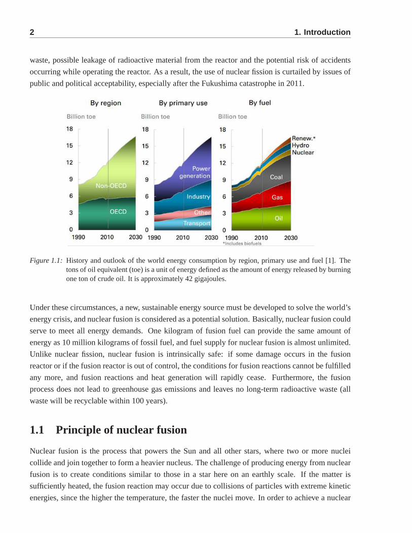
Other than renewable energy, nuclear fission is a controversial option for the energy supply, and it
satisfies about 5% of the world’s energy demand. As it is shownin figure 1.1, a large portion of
the increase in energy consumption is driven by power generation, in which nuclear fission plays a
very important role. Nuclear fission provides about 11% of the world’s electricity and almost 22%
of the electricity in OECD countries. Greenhouse gas emissions of nuclear power plants are among
the lowest of any electricity generation method, since nuclear power plants do not release any gases
such as carbon dioxide or methane which are largely responsible for the greenhouse effect. Nuclear
fission is reliable and efficient. Nuclear energy can be produced from nuclear power plants even
under rough weather conditions - and it needs only a small amount of fuel compared to producing
the same amount of energy by relying on fossil fuel. However,the disadvantages of nuclear fission
are obvious as well, e.g. the safety issues during transportof nuclear materials, disposal of nuclear
2 1. Introduction
waste, possible leakage of radioactive material from the reactor and the potential risk of accidents
occurring while operating the reactor. As a result, the use of nuclear fission is curtailed by issues of
public and political acceptability, especially after the Fukushima catastrophe in 2011.
Figure 1.1: History and outlook of the world energy consumption by region, primary useand fuel [1]. Thetons of oil equivalent (toe) is a unit of energy defined as the amount of energy released by burningone ton of crude oil. It is approximately 42 gigajoules.
Under these circumstances, a new, sustainable energy source must be developed to solve the world’s
energy crisis, and nuclear fusion is considered as a potential solution. Basically, nuclear fusion could
serve to meet all energy demands. One kilogram of fusion fuelcan provide the same amount of
energy as 10 million kilograms of fossil fuel, and fuel supply for nuclear fusion is almost unlimited.
Unlike nuclear fission, nuclear fusion is intrinsically safe: if some damage occurs in the fusion
reactor or if the fusion reactor is out of control, the conditions for fusion reactions cannot be fulfilled
any more, and fusion reactions and heat generation will rapidly cease. Furthermore, the fusion
process does not lead to greenhouse gas emissions and leavesno long-term radioactive waste (all
waste will be recyclable within 100 years).
1.1 Principle of nuclear fusion
Nuclear fusion is the process that powers the Sun and all other stars, where two or more nuclei
collide and join together to form a heavier nucleus. The challenge of producing energy from nuclear
fusion is to create conditions similar to those in a star hereon an earthly scale. If the matter is
sufficiently heated, the fusion reaction may occur due to collisions of particles with extreme kinetic
energies, since the higher the temperature, the faster the nuclei move. In order to achieve a nuclear
1.1. Principle of nuclear fusion 3
fusion reaction, it is necessary to heat up these nuclei to extremely high temperature of nearly 150
million degrees Celsius. At such extremely high temperatures, electrons are separated from nuclei,
forming a hot, electrically charged gas (plasma). If this condition can be maintained long enough
(e.g. a couple of seconds), the nuclei will be held together for nuclear fusion to occur. The mass
of the resulting heavier nucleus is not the exact sum of the two initial nuclei, and huge energy
quantities are released when the average mass of the nuclei involved in the process decreases. The
quantity of released energy relates to Einstein’s famous equation, which states that the universal
proportionality factor between equivalent amounts of energy and mass is equal to the speed of light
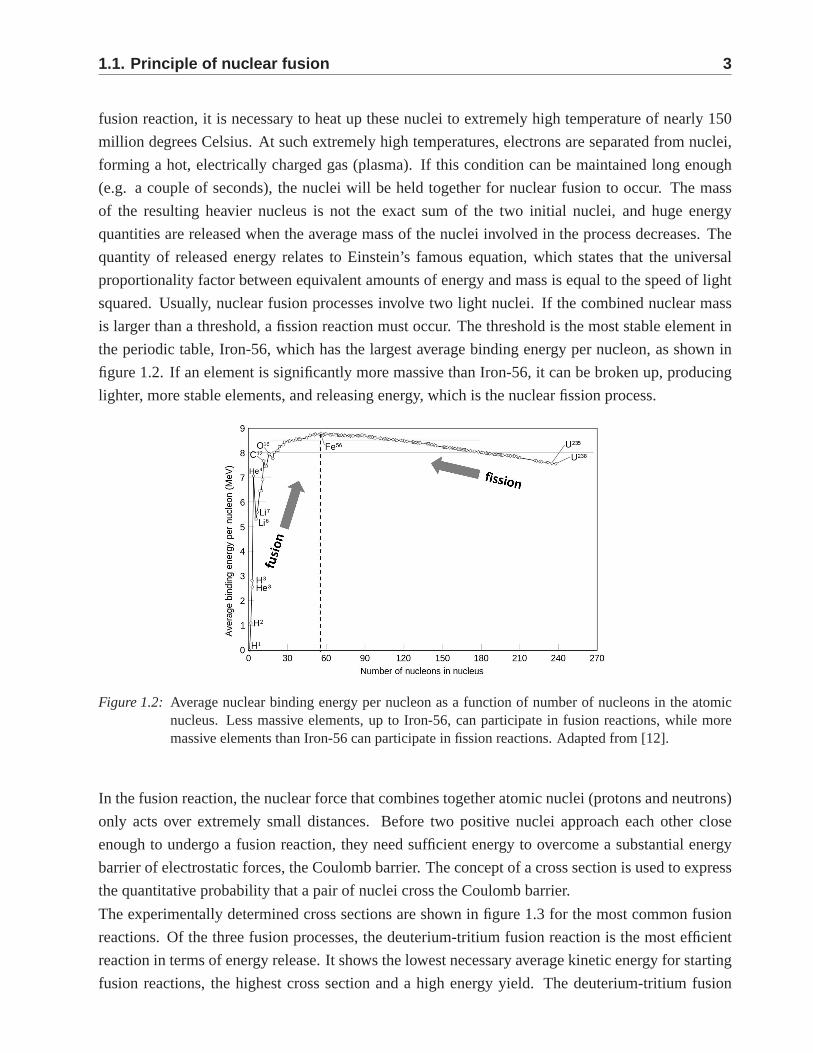
squared. Usually, nuclear fusion processes involve two light nuclei. If the combined nuclear mass
is larger than a threshold, a fission reaction must occur. Thethreshold is the most stable element in
the periodic table, Iron-56, which has the largest average binding energy per nucleon, as shown in
figure 1.2. If an element is significantly more massive than Iron-56, it can be broken up, producing
lighter, more stable elements, and releasing energy, whichis the nuclear fission process.
Figure 1.2: Average nuclear binding energy per nucleon as a function of number ofnucleons in the atomicnucleus. Less massive elements, up to Iron-56, can participate in fusion reactions, while moremassive elements than Iron-56 can participate in fission reactions. Adaptedfrom [12].
In the fusion reaction, the nuclear force that combines together atomic nuclei (protons and neutrons)
only acts over extremely small distances. Before two positive nuclei approach each other close
enough to undergo a fusion reaction, they need sufficient energy to overcome a substantial energy
barrier of electrostatic forces, the Coulomb barrier. The concept of a cross section is used to express
the quantitative probability that a pair of nuclei cross theCoulomb barrier.
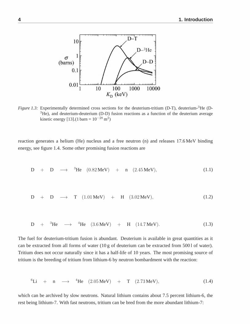
The experimentally determined cross sections are shown in figure 1.3 for the most common fusion
reactions. Of the three fusion processes, the deuterium-tritium fusion reaction is the most efficient
reaction in terms of energy release. It shows the lowest necessary average kinetic energy for starting
fusion reactions, the highest cross section and a high energy yield. The deuterium-tritium fusion
4 1. Introduction
Figure 1.3: Experimentally determined cross sections for the deuterium-tritium (D-T), deuterium-3He (D-3He), and deuterium-deuterium (D-D) fusion reactions as a function of thedeuterium averagekinetic energy [13].(1 barn = 10−28 m2)
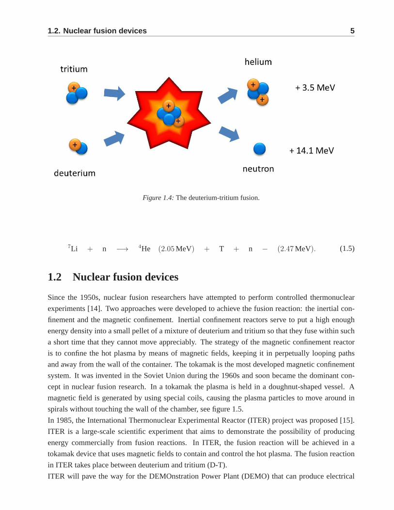
reaction generates a helium (He) nucleus and a free neutron (n) and releases 17.6 MeV binding
energy, see figure 1.4. Some other promising fusion reactions are
D + D −→ 3He (0.82 MeV) + n (2.45 MeV), (1.1)
D + D −→ T (1.01 MeV) + H (3.02 MeV), (1.2)
D + 3He −→ 4He (3.6 MeV) + H (14.7 MeV). (1.3)
The fuel for deuterium-tritium fusion is abundant. Deuterium is available in great quantities as it
can be extracted from all forms of water (10 g of deuterium canbe extracted from 500 l of water).
Tritium does not occur naturally since it has a half-life of 10 years. The most promising source of
tritium is the breeding of tritium from lithium-6 by neutronbombardment with the reaction:
6Li + n −→ 4He (2.05 MeV) + T (2.73 MeV), (1.4)
which can be archived by slow neutrons. Natural lithium contains about 7.5 percent lithium-6, the
rest being lithium-7. With fast neutrons, tritium can be bred from the more abundant lithium-7:
1.2. Nuclear fusion devices 5
Figure 1.4: The deuterium-tritium fusion.
7Li + n −→ 4He (2.05 MeV) + T + n − (2.47 MeV). (1.5)
1.2 Nuclear fusion devices
Since the 1950s, nuclear fusion researchers have attemptedto perform controlled thermonuclear
experiments [14]. Two approaches were developed to achievethe fusion reaction: the inertial con-
finement and the magnetic confinement. Inertial confinement reactors serve to put a high enough
energy density into a small pellet of a mixture of deuterium and tritium so that they fuse within such
a short time that they cannot move appreciably. The strategyof the magnetic confinement reactor
is to confine the hot plasma by means of magnetic fields, keeping it in perpetually looping paths
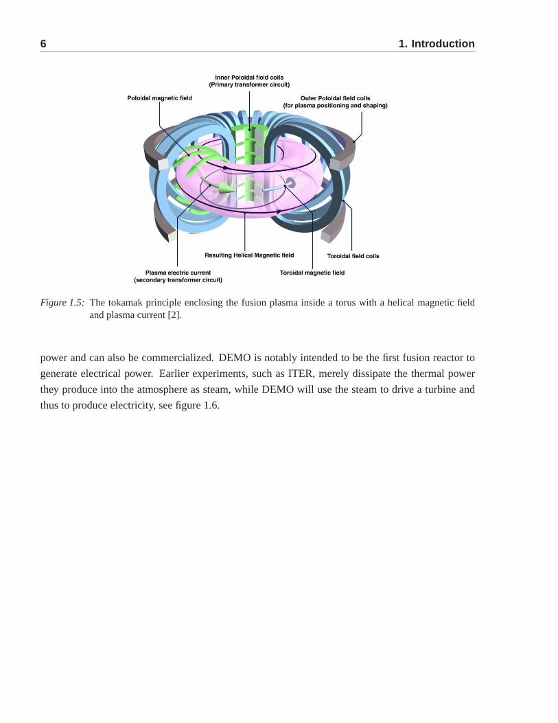
and away from the wall of the container. The tokamak is the most developed magnetic confinement
system. It was invented in the Soviet Union during the 1960s and soon became the dominant con-
cept in nuclear fusion research. In a tokamak the plasma is held in a doughnut-shaped vessel. A
magnetic field is generated by using special coils, causing the plasma particles to move around in
spirals without touching the wall of the chamber, see figure 1.5.
In 1985, the International Thermonuclear Experimental Reactor (ITER) project was proposed [15].
ITER is a large-scale scientific experiment that aims to demonstrate the possibility of producing
energy commercially from fusion reactions. In ITER, the fusion reaction will be achieved in a
tokamak device that uses magnetic fields to contain and control the hot plasma. The fusion reaction
in ITER takes place between deuterium and tritium (D-T).
ITER will pave the way for the DEMOnstration Power Plant (DEMO) that can produce electrical
6 1. Introduction
Figure 1.5: The tokamak principle enclosing the fusion plasma inside a torus with a helical magnetic fieldand plasma current [2].
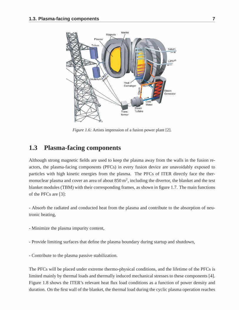
power and can also be commercialized. DEMO is notably intended to be the first fusion reactor to
generate electrical power. Earlier experiments, such as ITER, merely dissipate the thermal power
they produce into the atmosphere as steam, while DEMO will use the steam to drive a turbine and
thus to produce electricity, see figure 1.6.
1.3. Plasma-facing components 7
Figure 1.6: Artists impression of a fusion power plant [2].
1.3 Plasma-facing components
Although strong magnetic fields are used to keep the plasma away from the walls in the fusion re-
actors, the plasma-facing components (PFCs) in every fusiondevice are unavoidably exposed to
particles with high kinetic energies from the plasma. The PFCs of ITER directly face the ther-
monuclear plasma and cover an area of about 850 m2, including the divertor, the blanket and the test
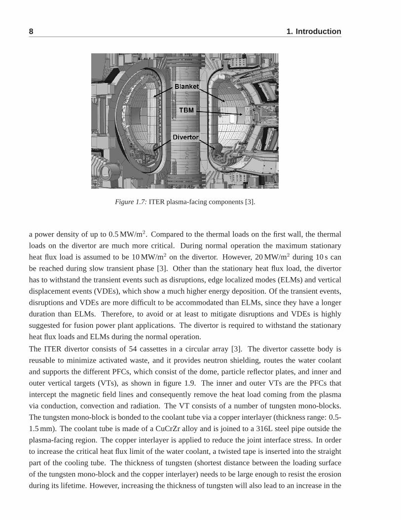
blanket modules (TBM) with their corresponding frames, as shown in figure 1.7. The main functions
of the PFCs are [3]:
- Absorb the radiated and conducted heat from the plasma and contribute to the absorption of neu-
tronic heating,
- Minimize the plasma impurity content,
- Provide limiting surfaces that define the plasma boundary during startup and shutdown,
- Contribute to the plasma passive stabilization.
The PFCs will be placed under extreme thermo-physical conditions, and the lifetime of the PFCs is
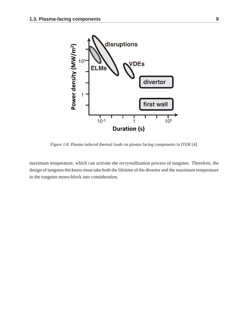
limited mainly by thermal loads and thermally induced mechanical stresses to these components [4].
Figure 1.8 shows the ITER’s relevant heat flux load conditionsas a function of power density and
duration. On the first wall of the blanket, the thermal load during the cyclic plasma operation reaches
8 1. Introduction
Figure 1.7: ITER plasma-facing components [3].
a power density of up to 0.5 MW/m2. Compared to the thermal loads on the first wall, the thermal
loads on the divertor are much more critical. During normal operation the maximum stationary
heat flux load is assumed to be 10 MW/m2 on the divertor. However, 20 MW/m2 during 10 s can
be reached during slow transient phase [3]. Other than the stationary heat flux load, the divertor
has to withstand the transient events such as disruptions, edge localized modes (ELMs) and vertical
displacement events (VDEs), which show a much higher energydeposition. Of the transient events,
disruptions and VDEs are more difficult to be accommodated than ELMs, since they have a longer
duration than ELMs. Therefore, to avoid or at least to mitigate disruptions and VDEs is highly
suggested for fusion power plant applications. The divertor is required to withstand the stationary
heat flux loads and ELMs during the normal operation.
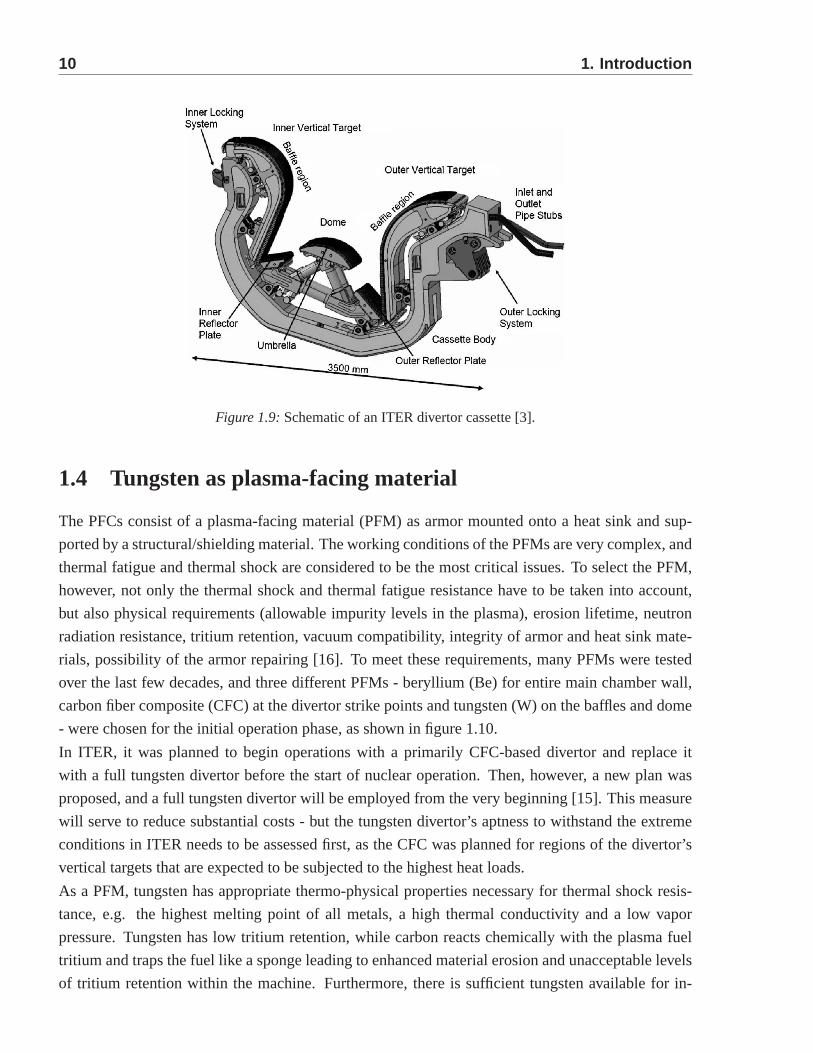
The ITER divertor consists of 54 cassettes in a circular array [3]. The divertor cassette body is
reusable to minimize activated waste, and it provides neutron shielding, routes the water coolant
and supports the different PFCs, which consist of the dome, particle reflector plates, and inner and
outer vertical targets (VTs), as shown in figure 1.9. The inner and outer VTs are the PFCs that
intercept the magnetic field lines and consequently remove the heat load coming from the plasma
via conduction, convection and radiation. The VT consists of a number of tungsten mono-blocks.
The tungsten mono-block is bonded to the coolant tube via a copper interlayer (thickness range: 0.5-
1.5 mm). The coolant tube is made of a CuCrZr alloy and is joined to a 316L steel pipe outside the
plasma-facing region. The copper interlayer is applied to reduce the joint interface stress. In order
to increase the critical heat flux limit of the water coolant,a twisted tape is inserted into the straight
part of the cooling tube. The thickness of tungsten (shortest distance between the loading surface
of the tungsten mono-block and the copper interlayer) needsto be large enough to resist the erosion
during its lifetime. However, increasing the thickness of tungsten will also lead to an increase in the
1.3. Plasma-facing components 9
Figure 1.8: Plasma induced thermal loads on plasma facing components in ITER [4].
maximum temperature, which can activate the recrystallization process of tungsten. Therefore, the
design of tungsten thickness must take both the lifetime of the divertor and the maximum temperature
in the tungsten mono-block into consideration.
10 1. Introduction
Figure 1.9: Schematic of an ITER divertor cassette [3].
1.4 Tungsten as plasma-facing material
The PFCs consist of a plasma-facing material (PFM) as armor mounted onto a heat sink and sup-
ported by a structural/shielding material. The working conditions of the PFMs are very complex, and
thermal fatigue and thermal shock are considered to be the most critical issues. To select the PFM,
however, not only the thermal shock and thermal fatigue resistance have to be taken into account,
but also physical requirements (allowable impurity levelsin the plasma), erosion lifetime, neutron
radiation resistance, tritium retention, vacuum compatibility, integrity of armor and heat sink mate-
rials, possibility of the armor repairing [16]. To meet these requirements, many PFMs were tested
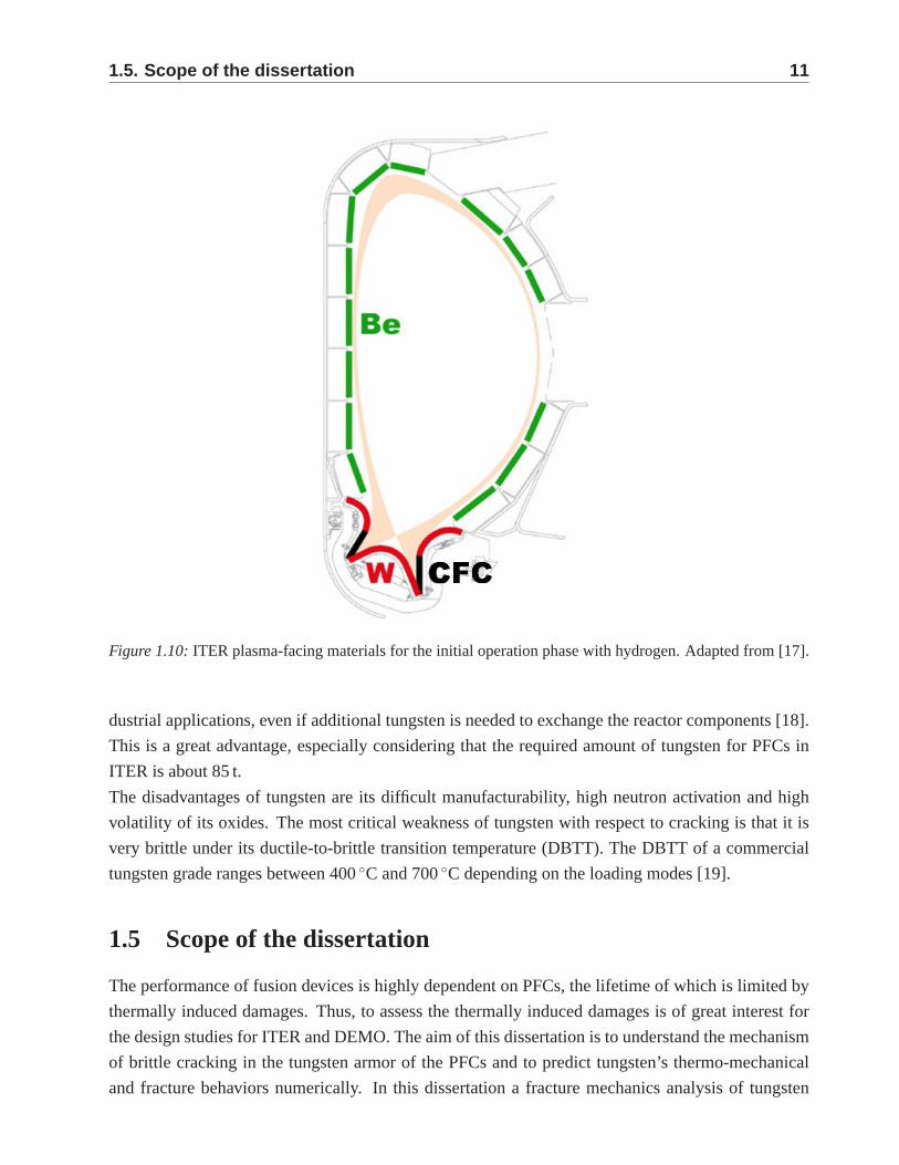
over the last few decades, and three different PFMs - beryllium (Be) for entire main chamber wall,
carbon fiber composite (CFC) at the divertor strike points and tungsten (W) on the baffles and dome
- were chosen for the initial operation phase, as shown in figure 1.10.
In ITER, it was planned to begin operations with a primarily CFC-based divertor and replace it
with a full tungsten divertor before the start of nuclear operation. Then, however, a new plan was
proposed, and a full tungsten divertor will be employed fromthe very beginning [15]. This measure
will serve to reduce substantial costs - but the tungsten divertor’s aptness to withstand the extreme
conditions in ITER needs to be assessed first, as the CFC was planned for regions of the divertor’s
vertical targets that are expected to be subjected to the highest heat loads.
As a PFM, tungsten has appropriate thermo-physical properties necessary for thermal shock resis-
tance, e.g. the highest melting point of all metals, a high thermal conductivity and a low vapor
pressure. Tungsten has low tritium retention, while carbonreacts chemically with the plasma fuel
tritium and traps the fuel like a sponge leading to enhanced material erosion and unacceptable levels
of tritium retention within the machine. Furthermore, there is sufficient tungsten available for in-
1.5. Scope of the dissertation 11
Figure 1.10: ITER plasma-facing materials for the initial operation phase with hydrogen. Adapted from [17].
dustrial applications, even if additional tungsten is needed to exchange the reactor components [18].
This is a great advantage, especially considering that the required amount of tungsten for PFCs in
ITER is about 85 t.
The disadvantages of tungsten are its difficult manufacturability, high neutron activation and high
volatility of its oxides. The most critical weakness of tungsten with respect to cracking is that it is
very brittle under its ductile-to-brittle transition temperature (DBTT). The DBTT of a commercial
tungsten grade ranges between 400◦C and 700◦C depending on the loading modes [19].
1.5 Scope of the dissertation
The performance of fusion devices is highly dependent on PFCs, the lifetime of which is limited by
thermally induced damages. Thus, to assess the thermally induced damages is of great interest for
the design studies for ITER and DEMO. The aim of this dissertation is to understand the mechanism
of brittle cracking in the tungsten armor of the PFCs and to predict tungsten’s thermo-mechanical
and fracture behaviors numerically. In this dissertation afracture mechanics analysis of tungsten
12 1. Introduction
failures is performed under three thermal loading scenarios - namely short transient thermal loads,
slow high-energy-deposition thermal loads and stationaryheat flux loads.
Short transient thermal loads
To mimic ITER-relevant short transient thermal loads (e.g. ELMs), electron beam facilities have
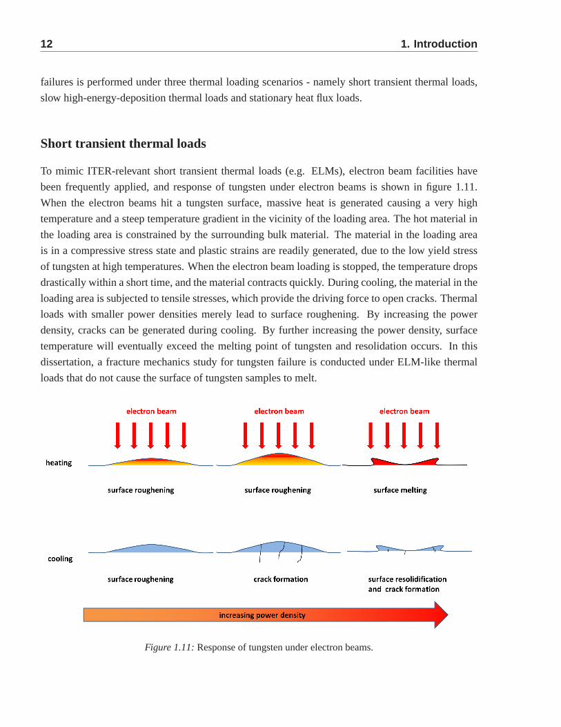
been frequently applied, and response of tungsten under electron beams is shown in figure 1.11.
When the electron beams hit a tungsten surface, massive heat is generated causing a very high
temperature and a steep temperature gradient in the vicinity of the loading area. The hot material in
the loading area is constrained by the surrounding bulk material. The material in the loading area
is in a compressive stress state and plastic strains are readily generated, due to the low yield stress
of tungsten at high temperatures. When the electron beam loading is stopped, the temperature drops
drastically within a short time, and the material contractsquickly. During cooling, the material in the
loading area is subjected to tensile stresses, which provide the driving force to open cracks. Thermal
loads with smaller power densities merely lead to surface roughening. By increasing the power
density, cracks can be generated during cooling. By further increasing the power density, surface
temperature will eventually exceed the melting point of tungsten and resolidation occurs. In this
dissertation, a fracture mechanics study for tungsten failure is conducted under ELM-like thermal
loads that do not cause the surface of tungsten samples to melt.
Figure 1.11: Response of tungsten under electron beams.
1.6. Outline 13
Slow high-energy-deposition thermal loads
Besides short transient thermal loads, the PFCs will be facingslow high-energy-deposition thermal
loads, which have a much longer duration. A typical example is to be seen in the VDE. The deposited
energy densities (60 MJ/m2) resulting from the VDE along with the long pulse duration, which is
nearly three magnitudes higher of the pulse duration of the ELMs, usually lead to the melting of
PFCs’ surface and the subsequent redistribution of the PFM. Melting of tungsten is beyond the
scope of this dissertation. However, the VDE is a uncontrolled scenario and its mechanism remains
unclear. If the thermal loading induced by the VDEs is limited to an area that is sufficiently small,
the temperature will not exceed the melting point of tungsten. In this dissertation, the behavior of
tungsten is studied under VDE-like thermal loads assuming the loading area is limited so that no
melting of tungsten occurs.
Stationary heat flux loads
The stationary heat flux load is not as intensive as thermal transient loads, and usually no plastic
deformation is generated in tungsten during the operation purely due to the stationary heat flux load.
However, the stationary heat flux loads impose a strong constraint on the structure-mechanical per-
formance of the divertor during the operation. Thus, the combination of brittleness and the thermally
induced stress fields due to the stationary heat flux loads raises a serious reliability issue concerning
the structural integrity of tungsten armor. In this dissertation, the failure of a water-cooled divertor
target is studied under ITER and DEMO relevant stationary heat flux loads.
1.6 Outline
This dissertation is organized as follows. Chapter 2 focuseson the theoretical background of the
fracture mechanics studies conducted in this dissertation, and the methods for calculating stress
intensity factors andJ-integrals are presented. Also, the principle of the extended finite element
method (XFEM) is introduced.
In chapter 3, a simplified analytical solution of temperature, stress and strain is derived under ELM-
like transient thermal loading in a semi-infinite space. Based on the analytical stress solution, stress
intensity factors are calculated by using the weight function method. In order to enable a more pre-
cise analysis, the finite element model is built according tothe setup of thermal shock experiments
at Forschungszentrum Julich. The fracture behavior of tungsten is studied by meansof two different
types of computational approaches, namely, XFEM and the FEM-based virtual crack tip extension
(VCE) method. A series of parametric simulations are conducted to study the impact of power den-
sity, base temperature and loading pattern on thermo-mechanical and fracture mechanical behaviors
of tungsten.
14 1. Introduction
Chapter 4 focuses on a numerical investigation of the thermo-mechanical and fracture behaviors
of tungsten under slow high-energy-deposition thermal loads. The maximum temperature, surface
roughness and crack occurrence are predicted and compared with the results of the thermal shock
experiments undertaken at Siemens Healthcare.
In chapter 5, an extensive finite element analysis of the fracture mechanical behavior of a tungsten
mono-block divertor target is carried out under consideration of ITER and DEMO relevant stationary
heat flux loading conditions.
In chapter 6, the conclusions drawn from this dissertation are presented and further improvements
of the current fracture mechanical simulations are proposed.
15
Chapter 2
Computational fracture mechanics
approaches
This chapter serves to describe the research methodology ofcomputing stress intensity factor,J-
integral, crack initiation and crack propagation. In this chapter, after a brief overview of the funda-
mental concepts of fracture mechanics, the principle of theweight function method is introduced.
The methods for computing stress intensity factor andJ-integral in the commercial FEM code
ABAQUS are described. In the end, the concept of XFEM to predict crack initiation and propa-
gation is explained.
2.1 Fundamental concepts of fracture mechanics
The brittle cracking of tungsten under thermal shocks is essentially related to the brittleness of tung-
sten at low temperatures. Thus, the fracture behavior of tungsten below DBTT can in principle be
interpreted with linear elastic fracture mechanics. The foundation of fracture mechanics, or more
specifically, the foundation of linear elastic fracture mechanics was laid in the 1920s by Griffith [20].
A material fractures when sufficient stress is applied at theatomic level to break the bonds that hold
atoms together. The strength is supplied by the attractive forces between atoms. In practice, how-
ever, it is found that the observed fracture strength is muchsmaller than the theoretical stress needed
for breaking atomic bonds. Griffith explained the discrepancy between observed fracture strength
and theoretical cohesive strength by inherent defects suchas pre-existing micro-cracks in brittle ma-
terials leading to stress concentration. But to calculate this stress based on linear elasticity theory is
problematic. Linear elasticity theory predicts that stress at the tip of a sharp flaw is infinite in a linear
elastic material. To avoid this problem, Griffith developeda fracture theory based on energy rather
than on local stress. The creation of a new crack surface absorbs energy that is supplied from the
work done by the external force - and the failure is promoted by a release of the stored strain energy
in the solid material, which is sufficient to overcome the resistance to crack propagation. This energy
16 2. Computational fracture mechanics approaches
per unit of newly created crack surface area defines an important parameter called the energy release
rate (or strain energy release rate), denoted byG in honor of Griffith. In the later computational
study in this dissertation, cracks are assumed to be initiated if the stress in the continuous mechanics
framework is higher than the fracture strength that is obtained from experiments. The released en-
ergy is used to determine the crack propagation.Gc is defined as the critical value of energy released
per unit length of crack extension. A crack is stable as long asG is smaller thanGc.
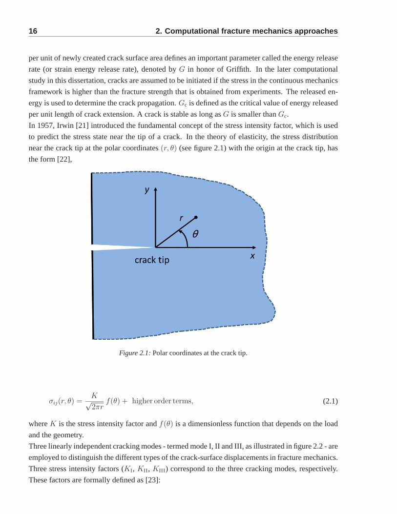
In 1957, Irwin [21] introduced the fundamental concept of the stress intensity factor, which is used
to predict the stress state near the tip of a crack. In the theory of elasticity, the stress distribution
near the crack tip at the polar coordinates(r, θ) (see figure 2.1) with the origin at the crack tip, has
the form [22],
Figure 2.1: Polar coordinates at the crack tip.
σij(r, θ) =K√2πr
f(θ) + higher order terms, (2.1)
whereK is the stress intensity factor andf(θ) is a dimensionless function that depends on the load
and the geometry.
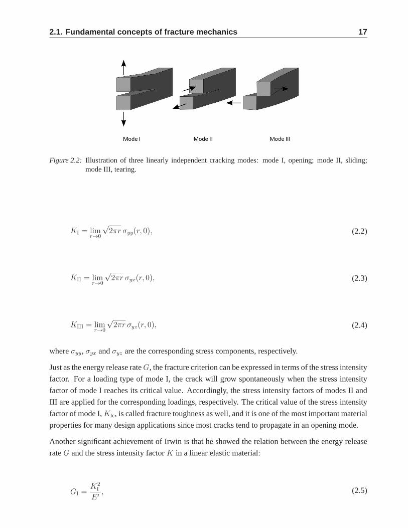
Three linearly independent cracking modes - termed mode I, II and III, as illustrated in figure 2.2 - are
employed to distinguish the different types of the crack-surface displacements in fracture mechanics.
Three stress intensity factors (KI, KII, KIII) correspond to the three cracking modes, respectively.
These factors are formally defined as [23]:
2.1. Fundamental concepts of fracture mechanics 17
Figure 2.2: Illustration of three linearly independent cracking modes: mode I, opening;mode II, sliding;mode III, tearing.
KI = limr→0
√2πr σyy(r, 0), (2.2)
KII = limr→0
√2πr σyx(r, 0), (2.3)
KIII = limr→0
√2πr σyz(r, 0), (2.4)
whereσyy, σyx andσyz are the corresponding stress components, respectively.
Just as the energy release rateG, the fracture criterion can be expressed in terms of the stress intensity
factor. For a loading type of mode I, the crack will grow spontaneously when the stress intensity
factor of mode I reaches its critical value. Accordingly, the stress intensity factors of modes II and
III are applied for the corresponding loadings, respectively. The critical value of the stress intensity
factor of mode I,KIc, is called fracture toughness as well, and it is one of the most important material
properties for many design applications since most cracks tend to propagate in an opening mode.
Another significant achievement of Irwin is that he showed the relation between the energy release
rateG and the stress intensity factorK in a linear elastic material:
GI =K2
I
E ′, (2.5)
18 2. Computational fracture mechanics approaches
GII =K2
II
E ′, (2.6)
GIII =K2
III
2µ, (2.7)
whereGI, GII andGIII are the energy release rates for mode I, mode II and mode III, respectively.
E ′ is the effective Young’s modulus, which equals to the Young’s modulus,E, for plane stress and
E/(1 − ν2) for plane strain, whereν is the Poisson’s ratio. The shear modulus,µ, can be obtained
by
µ =E
2(1 + ν). (2.8)
In the mid-1960s, the concept of theJ-integral was developed by James R. Rice [24]. For isotropic,
linear elastic materials, theJ-integral is equal to the energy release rate, which provides a way to
evaluate the energy release rate for Griffith’s theory. TheJ-integral is a contour integral around
the crack tip, which is proven to be path independent in both linear elastic and non-linear elastic
materials. Furthermore, the path independence of theJ-integral rigorously holds in elasto-plastic
materials when the monotonic loading is applied. The path independence of theJ-integral avoids
difficulties involved in computing the stress close to a crack in a nonlinear elastic or elasto-plastic
material.
2.2 Weight function method
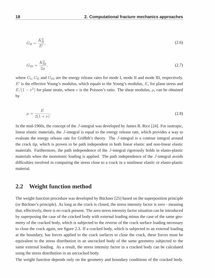
The weight function procedure was developed by Buckner [25] based on the superposition principle
(or Buckner’s principle). As long as the crack is closed, the stress intensity factor is zero - meaning
that, effectively, there is no crack present. The zero stress intensity factor situation can be introduced
by superposing the case of the cracked body with external loading minus the case of the same geo-
metry of the cracked body, which is subjected to the reverse of the crack surface loading necessary
to close the crack again, see figure 2.3. If a cracked body, which is subjected to an external loading
at the boundary, has forces applied to the crack surfaces to close the crack, these forces must be
equivalent to the stress distribution in an uncracked body of the same geometry subjected to the
same external loading. As a result, the stress intensity factor in a cracked body can be calculated
using the stress distribution in an uncracked body.
The weight function depends only on the geometry and boundary conditions of the cracked body.
2.2. Weight function method 19
Figure 2.3: Illustration of the superposition principle used for the weight function method.
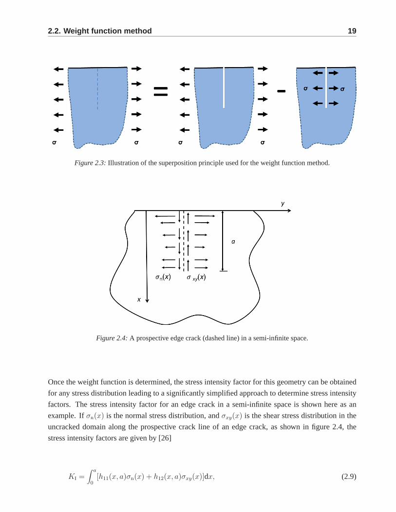
Figure 2.4: A prospective edge crack (dashed line) in a semi-infinite space.
Once the weight function is determined, the stress intensity factor for this geometry can be obtained
for any stress distribution leading to a significantly simplified approach to determine stress intensity
factors. The stress intensity factor for an edge crack in a semi-infinite space is shown here as an
example. Ifσn(x) is the normal stress distribution, andσxy(x) is the shear stress distribution in the
uncracked domain along the prospective crack line of an edgecrack, as shown in figure 2.4, the
stress intensity factors are given by [26]
KI =∫ a
0[h11(x, a)σn(x) + h12(x, a)σxy(x)]dx, (2.9)
20 2. Computational fracture mechanics approaches
KII =∫ a
0[h21(x, a)σn(x) + h22(x, a)σxy(x)]dx, (2.10)
whereh11, h21, h12, h22 are the weight functions, anda is the crack length. In most practical cases,
h21 andh12 disappear, and a simple form is obtained:
KI =∫ a
0h11(x, a)σn(x)dx, (2.11)
KII =∫ a
0h22(x, a)σxy(x)dx. (2.12)
There are handbooks that list the according weight functions, derived analytically or numerically for
cases of simple loading. The weight functionh(x, a) for edge cracks in a semi-infinite space with a
normal stress distribution only along the prospective crack line is given by [27]
h(x, a) =2
√
2π(a − x)[1 + M1(1 − x
a)
1
2 + M2(1 − x
a)1 + M3(1 − x
a)
3
2 ], (2.13)
whereM1 = 0.0719768,M2 = 0.246984 andM3 = 0.514465.
2.3 ComputingJ-integral and stress intensity factor [11]
2.3.1 J-integral
Under quasi-static conditions and in the absence of body forces, thermal strains and crack face
traction, the path independentJ-integral is written as follows [24]:
J = limΓ→0
∫
Γ[Wδ1i − σij
∂uj
∂x1
]nidΓ, (2.14)
whereΓ is the contour surrounding a crack tip,ni is the component of the outward normal unit
vector,n, to Γ andW is the strain energy density.σij anduj denote the Cartesian components of
the stress and displacement, respectively.x1 is the Cartesian coordinate parallel to the crack and
x2 is the Cartesian coordinate perpendicular to the crack. Shihet al. extended the original contour
integral formulation of theJ-integral to the domain integral expression [28]. In the absence of body
forces and crack face traction but in presence of thermal strains, this can be written as follows:
2.3. Computing J-integral and stress intensity factor [11] 21
J =∫
A{[σij
∂uj
∂x1
− Wδ1i]∂q1
∂x1
+ [ασii
∂∆T
∂x1
]q1}dA, (2.15)
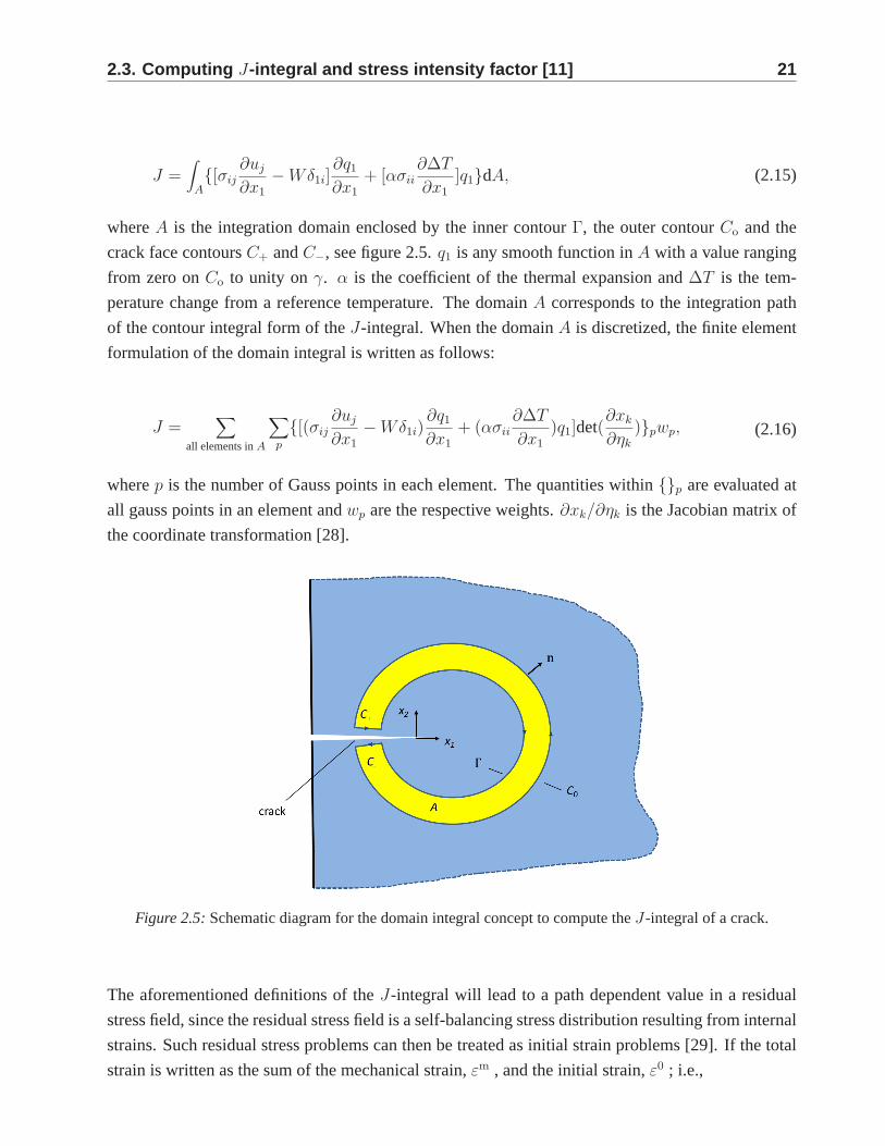
whereA is the integration domain enclosed by the inner contourΓ, the outer contourCo and the
crack face contoursC+ andC−, see figure 2.5.q1 is any smooth function inA with a value ranging
from zero onCo to unity onγ. α is the coefficient of the thermal expansion and∆T is the tem-
perature change from a reference temperature. The domainA corresponds to the integration path
of the contour integral form of theJ-integral. When the domainA is discretized, the finite element
formulation of the domain integral is written as follows:
J =∑
all elements inA
∑
p
{[(σij
∂uj
∂x1
− Wδ1i)∂q1
∂x1
+ (ασii
∂∆T
∂x1
)q1]det(∂xk
∂ηk
)}pwp, (2.16)
wherep is the number of Gauss points in each element. The quantitieswithin {}p are evaluated at
all gauss points in an element andwp are the respective weights.∂xk/∂ηk is the Jacobian matrix of
the coordinate transformation [28].
Figure 2.5: Schematic diagram for the domain integral concept to compute theJ-integral of a crack.
The aforementioned definitions of theJ-integral will lead to a path dependent value in a residual
stress field, since the residual stress field is a self-balancing stress distribution resulting from internal
strains. Such residual stress problems can then be treated as initial strain problems [29]. If the total
strain is written as the sum of the mechanical strain,εm , and the initial strain,ε0 ; i.e.,
22 2. Computational fracture mechanics approaches
ε = εm + ε0, (2.17)
the path-independentJ-integral in the presence of a residual stress field is given by [29]
J =∫
A{[σij
∂uj
∂x1
− Wδ1i]∂q1
∂x1
+ σij
∂ε0ij
∂x1
q1}dA, (2.18)
whereW is defined as the mechanical strain energy density:
W =∫ εm
0σ : dεm. (2.19)
whereσσσ is the stress tensor. The initial strainε0 remains constant during the entire deformation.
Within the finite element framework, theJ-integral expression is given by [29]
J =∑
all elements inA
∑
p
{[(σij
∂uj
∂x1
− Wδ1i)∂q1
∂x1
+ σij
∂ε0ij
∂x1
q1]det(∂xk
∂ηk
)}pwp. (2.20)
2.3.2 Stress intensity factor
In ABAQUS, stress intensity factors are calculated based onthe interaction integral method, which
is an effective tool for calculating mixed-mode fracture parameters in homogeneous materials [30].
In general, theJ-integral for a given problem can be written as
J =1
8π[KIB
−111 KI + 2KIB
−112 KII + 2KIB
−113 KIII + (terms not involvingKI)], (2.21)
whereB is the pre-logarithmic energy factor matrix. For an auxiliary and pure mode I specific crack
tip field, theJ-integral is defined by stress intensity factorkI as
J Iaux =
1
8πkI · B−1
11 · kI. (2.22)
Superimposing the auxiliary field onto the actual field yields
J Itot =
1
8π[(KI + kI)B
−111 (KI + kI) + 2(KI + kI)B
−112 KII + 2(KI + kI)B
−113 KIII
+(terms not involvingKI or kI)].(2.23)
2.4. Extended finite element method 23
Since the terms that do not involveKI or kI are identical inJ Itot andJ , the interaction integral can
be defined as
J Iint = J I
tot − J − J Iaux =
kI
4π[B−1
11 KI + B−112 KII + B−1
13 KIII]. (2.24)
If the calculations are repeated for mode II and mode III, a system of linear equations is obtained:
Jαint =
kα
4πB−1
αβ Kβ, (2.25)
whereα andβ represent the index of I, II and III. No summation is made onα = I, II, III. I, II and
III correspond to 1,2 and 3 when indicating the components ofB.
If kα are assigned the value 1, the solution of the above equationsleads to
K = 4πB · Jint, (2.26)
whereJint = [J Iint, J II
int, J IIIint ]
T . Based on the definition of theJ-integral, the interaction integrals
Jαint can be expressed as
Jαint = lim
Γ→0
∫
Γn · (σ : εα
auxI − σ · (∂u∂x
)αaux − σα
aux · ∂u∂x
) · q dΓ, (2.27)
whereI is the identity matrix,u is the displacement vector,x is the coordinate vector andq is referred
to as the crack-extension vector. The subscript aux represents three auxiliary pure mode I, mode II
and mode III crack tip fields forα = I, II, III, respectively.
2.4 Extended finite element method
2.4.1 Discontinuity modeling
The extended finite element method developed by Belytschko and Black [31] is a method whereby
crack initiation and growth can be modelled by the finite element method without remeshing. The
essential idea of this method is to introduce enrichment functions to describe a discontinuous dis-
placement field. It is an extension of the conventional finiteelement method based on the concept of
partition of unity by Melenk and Babuska [32], which allows local enrichment functions to be easily
incorporated into a finite element approximation. The presence of discontinuities is ensured by the
special enriched functions in conjunction with additionaldegrees of freedom.
XFEM is implemented in ABAQUS from version 6.9 onwards. For the purpose of a fracture me-
chanics analysis, the enrichment functions typically consist of the near-tip asymptotic functions that
24 2. Computational fracture mechanics approaches
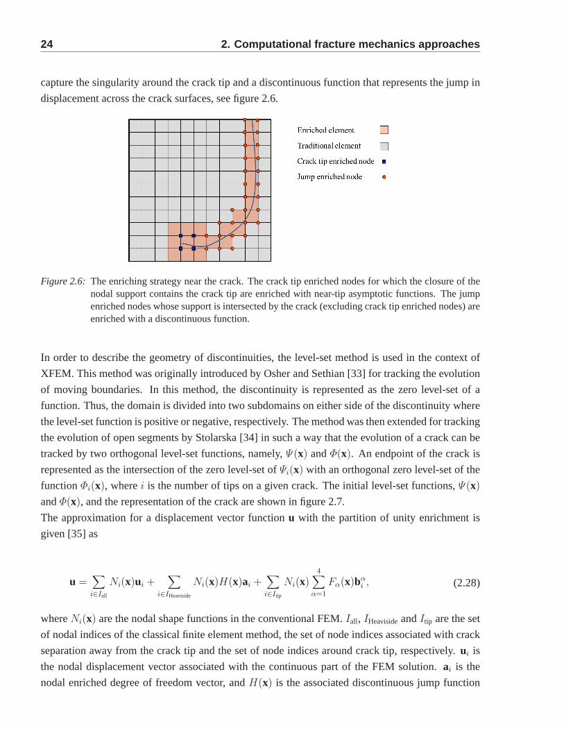
capture the singularity around the crack tip and a discontinuous function that represents the jump in
displacement across the crack surfaces, see figure 2.6.
Figure 2.6: The enriching strategy near the crack. The crack tip enriched nodes for which the closure of thenodal support contains the crack tip are enriched with near-tip asymptotic functions. The jumpenriched nodes whose support is intersected by the crack (excluding crack tip enriched nodes) areenriched with a discontinuous function.
In order to describe the geometry of discontinuities, the level-set method is used in the context of
XFEM. This method was originally introduced by Osher and Sethian [33] for tracking the evolution
of moving boundaries. In this method, the discontinuity is represented as the zero level-set of a
function. Thus, the domain is divided into two subdomains oneither side of the discontinuity where
the level-set function is positive or negative, respectively. The method was then extended for tracking
the evolution of open segments by Stolarska [34] in such a waythat the evolution of a crack can be
tracked by two orthogonal level-set functions, namely,Ψ(x) andΦ(x). An endpoint of the crack is
represented as the intersection of the zero level-set ofΨi(x) with an orthogonal zero level-set of the
functionΦi(x), wherei is the number of tips on a given crack. The initial level-set functions,Ψ(x)
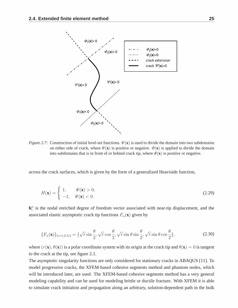
andΦ(x), and the representation of the crack are shown in figure 2.7.
The approximation for a displacement vector functionu with the partition of unity enrichment is
given [35] as
u =∑
i∈Iall
Ni(x)ui +∑
i∈IHeaviside
Ni(x)H(x)ai +∑
i∈Itip
Ni(x)4
∑
α=1
Fα(x)bαi , (2.28)
whereNi(x) are the nodal shape functions in the conventional FEM.Iall, IHeavisideandItip are the set
of nodal indices of the classical finite element method, the set of node indices associated with crack
separation away from the crack tip and the set of node indicesaround crack tip, respectively.ui is
the nodal displacement vector associated with the continuous part of the FEM solution.ai is the
nodal enriched degree of freedom vector, andH(x) is the associated discontinuous jump function
2.4. Extended finite element method 25
Figure 2.7: Construction of initial level-set functions.Ψ(x) is used to divide the domain into two subdomainson either side of crack, whereΨ(x) is positive or negative.Φ(x) is applied to divide the domaininto subdomains that is in front of or behind crack tip, whereΦ(x) is positive or negative.
across the crack surfaces, which is given by the form of a generalized Heaviside function,
H(x) =
1, Ψ(x) > 0,
−1, Ψ(x) < 0.(2.29)
bαi is the nodal enriched degree of freedom vector associated with near-tip displacement, and the
associated elastic asymptotic crack tip functionsFα(x) given by
{Fα(x)}α=1,2,3,4 = {√
r sinθ
2,√
r cosθ
2,√
r sin θ sinθ
2,√
r sin θ cosθ
2}, (2.30)
where(r(x), θ(x)) is a polar coordinate system with its origin at the crack tip andθ(x) = 0 is tangent
to the crack at the tip, see figure 2.1.
The asymptotic singularity functions are only considered for stationary cracks in ABAQUS [11]. To
model progressive cracks, the XFEM-based cohesive segments method and phantom nodes, which
will be introduced later, are used. The XFEM-based cohesivesegments method has a very general
modeling capability and can be used for modeling brittle or ductile fracture. With XFEM it is able
to simulate crack initiation and propagation along an arbitrary, solution-dependent path in the bulk
26 2. Computational fracture mechanics approaches
materials, since crack propagation is not tied to the element boundaries in a mesh. In this case,
the near-tip asymptotic singularity is not needed, and onlythe displacement jump across a cracked
element is considered. Therefore, the crack has to propagate across an entire element at a time to
avoid the necessity of modeling the stress singularity.
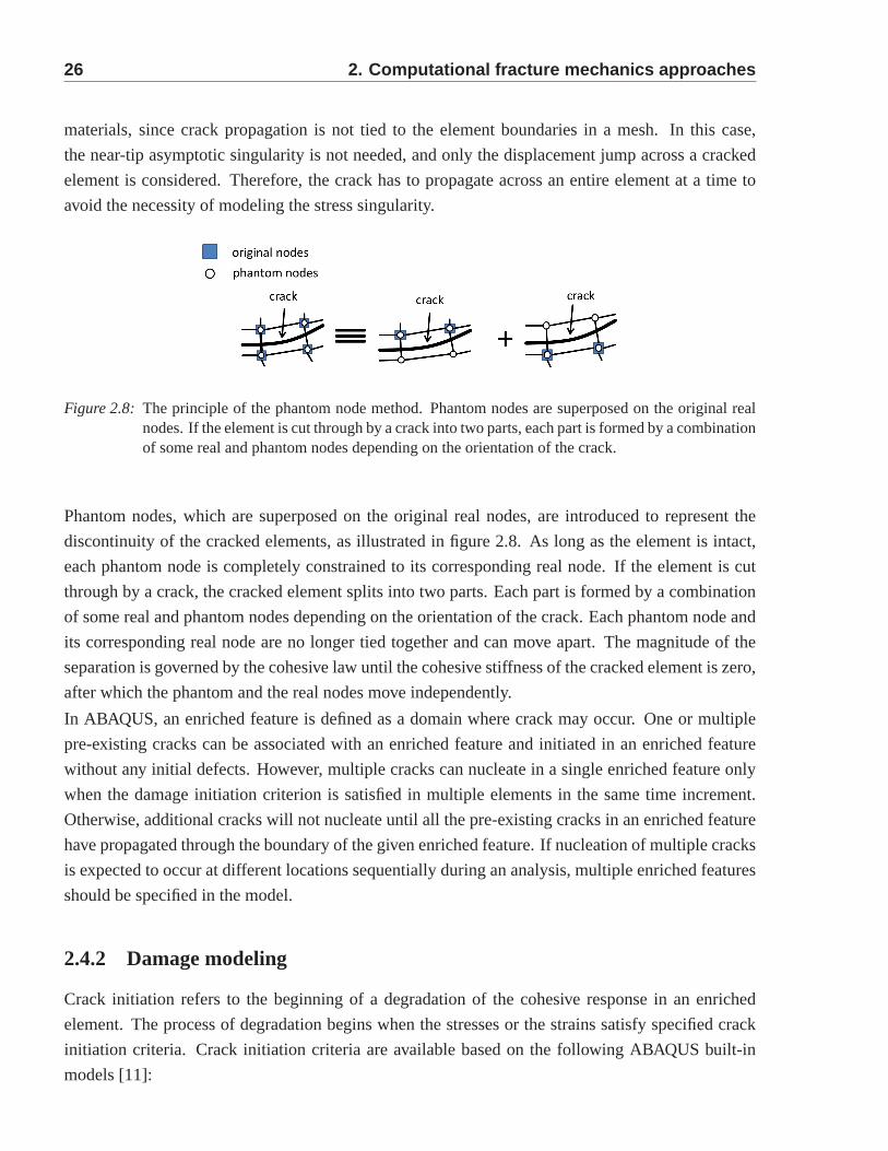
Figure 2.8: The principle of the phantom node method. Phantom nodes are superposed on the original realnodes. If the element is cut through by a crack into two parts, each part isformed by a combinationof some real and phantom nodes depending on the orientation of the crack.
Phantom nodes, which are superposed on the original real nodes, are introduced to represent the
discontinuity of the cracked elements, as illustrated in figure 2.8. As long as the element is intact,
each phantom node is completely constrained to its corresponding real node. If the element is cut
through by a crack, the cracked element splits into two parts. Each part is formed by a combination
of some real and phantom nodes depending on the orientation of the crack. Each phantom node and
its corresponding real node are no longer tied together and can move apart. The magnitude of the
separation is governed by the cohesive law until the cohesive stiffness of the cracked element is zero,
after which the phantom and the real nodes move independently.
In ABAQUS, an enriched feature is defined as a domain where crack may occur. One or multiple
pre-existing cracks can be associated with an enriched feature and initiated in an enriched feature
without any initial defects. However, multiple cracks can nucleate in a single enriched feature only
when the damage initiation criterion is satisfied in multiple elements in the same time increment.
Otherwise, additional cracks will not nucleate until all the pre-existing cracks in an enriched feature
have propagated through the boundary of the given enriched feature. If nucleation of multiple cracks
is expected to occur at different locations sequentially during an analysis, multiple enriched features
should be specified in the model.
2.4.2 Damage modeling
Crack initiation refers to the beginning of a degradation of the cohesive response in an enriched
element. The process of degradation begins when the stresses or the strains satisfy specified crack
initiation criteria. Crack initiation criteria are available based on the following ABAQUS built-in
models [11]:
2.4. Extended finite element method 27
• the maximum principal stress criterion,
• the maximum principal strain criterion,
• the maximum nominal stress criterion,
• the maximum nominal strain criterion.
In this dissertation, the maximum principal stress (MPS) criterion is applied. When the criterion is
satisfied,
〈σmax〉 ≥ σ0max, (2.31)
whereσ0max represents the maximum allowable principal stress, the resulting crack is always orthog-
onal to the maximum principal stress direction. The symbol〈〉 represents the Macaulay bracket with
the usual interpretation (i.e.,〈σmax〉 = 0 if σmax < 0, and〈σmax〉 = σmax if σmax ≥ 0). The enriched
elements do not, therefore, undergo damage under pure compression.
The cohesive material behavior is applied to the cracked domain in XFEM simulations. The elastic
behavior is written in terms of an elastic constitutive matrix that relates the normal and shear stresses
to the normal and shear separations of a cracked element. Theelastic behavior can then be written
as
t =
tn
ts
tt
=
Knn 0 0
0 Kss 0
0 0 Ktt
δn
δs
δt
= Kδ, (2.32)
where the nominal traction stress vector,t, consists of the components:tn, ts and (in three-dimensional
problems)tt, which represent the normal and the two shear tractions, respectively.δn, δs, andδt de-
note the corresponding separations. The termsKnn, Kss andKtt are stiffnesses calculated for an
enriched element based on the elastic properties.
The normal and tangential stiffness components will not be coupled, since pure normal separation
by itself does not give rise to cohesive forces in the shear directions, and pure shear slip with zero
normal separation does not give rise to any cohesive forces in the normal direction. Once a damage
initiation criterion is met, damage can occur according to auser-defined damage evolution law, as
shown in figure 2.9.
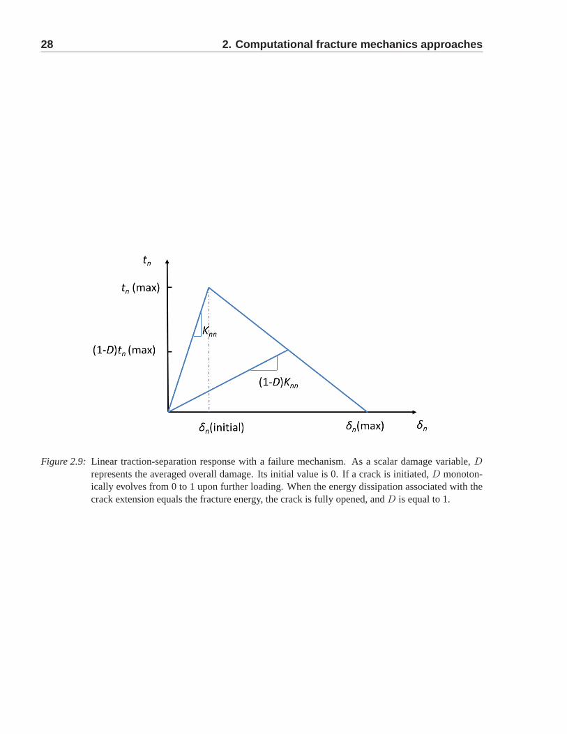
28 2. Computational fracture mechanics approaches
Figure 2.9: Linear traction-separation response with a failure mechanism. As a scalar damage variable,Drepresents the averaged overall damage. Its initial value is 0. If a crackis initiated,D monoton-ically evolves from 0 to 1 upon further loading. When the energy dissipation associated with thecrack extension equals the fracture energy, the crack is fully opened,andD is equal to 1.
29
Chapter 3
Fracture mechanics analysis of tungsten
under short transient thermal loads by
ELMs
3.1 Edge localized modes
Fortunately, it was discovered during the ASDEX tokamak experiments at Max Planck Institute for
Plasma Physics in Garching, Germany, that certain conditions during the application of neutral beam
injection heating lead to a transition to a high confinement mode (H-mode) [36]. The plasma en-
ergy confinement time of the H-mode is nearly twice that of thelow confinement mode (L-mode).
This discovery is to be seen as an important step to reaching higher temperatures and pressures in
tokamaks. Today, almost all tokamaks, including the tokamaks in ITER and DEMO, are designed
to operate in H-mode. However, in addition to the increase inconfinement time, a new type of in-
stability, called edge localized mode (ELM), was found. As aconsequence of the ELM instability, a
steep plasma pressure gradient is formed at the edge of the plasma. Figure 3.1 shows the magnetic
geometry of a divertor tokamak and pressure profiles of L- andH-mode plasmas. The plasma pres-
sure profile at the plasma edge relaxes periodically towardsless steep slopes (ELM crash). Then, it
steepens again before collapsing at the following ELM (ELM recovery). As a consequence, energy
and particles are released into the Scrape-Off-Layer (SOL)in a very short timescale,<1 ms [37]. In
a standard H-mode plasma, ELMs occur repetitively, and the energy lost from inside the separatrix
that flows along field lines into the divertor results in an ELMheat flux pulse. Regarding the heating
power dependence of the ELM frequency and the theoretical peeling-ballooning stability limit, three
types of ELMs (type-I, type-II and type-III) were classifiedand are commonly accepted [37]. Of
the three modes, the type I ELMs can cause the most significantdamage in PFMs. Although several
methods (e.g. radiating divertors [38], magnetic triggering [39], pellet pace-making of ELMs [40],
edge ergodisation [41, 42]) have been applied to control ELMs, some unexpected ELMs can still
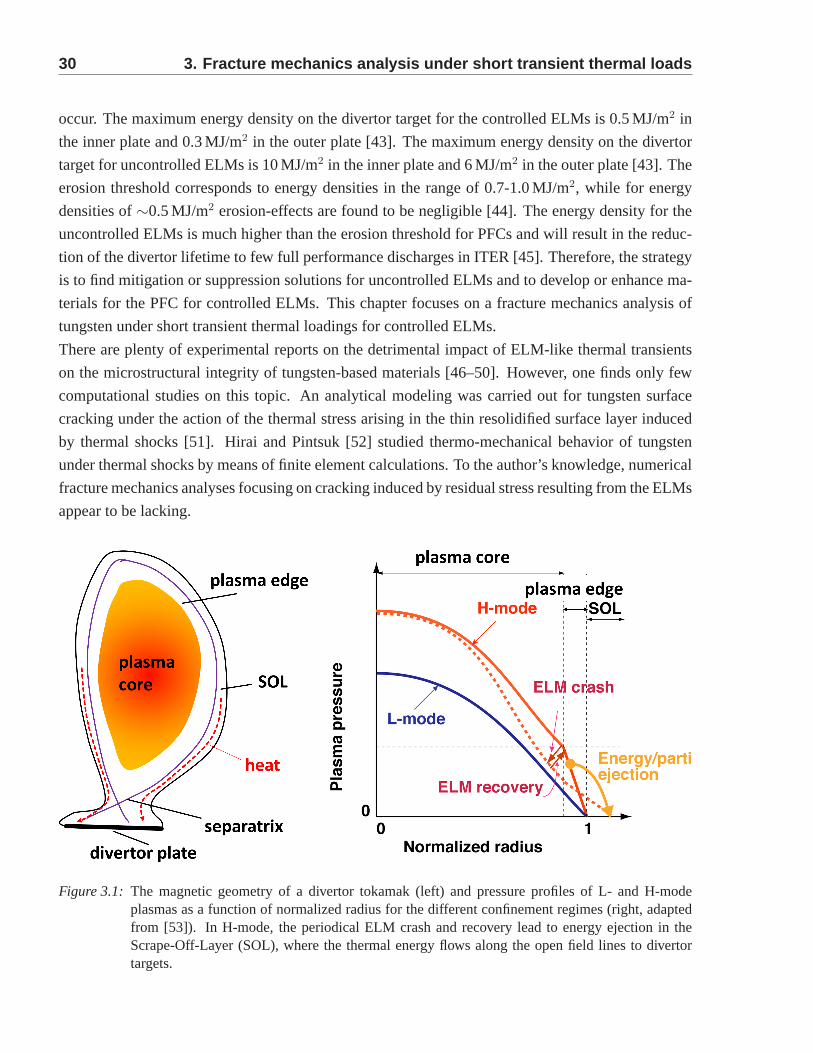
30 3. Fracture mechanics analysis under short transient the rmal loads
occur. The maximum energy density on the divertor target forthe controlled ELMs is 0.5 MJ/m2 in
the inner plate and 0.3 MJ/m2 in the outer plate [43]. The maximum energy density on the divertor
target for uncontrolled ELMs is 10 MJ/m2 in the inner plate and 6 MJ/m2 in the outer plate [43]. The
erosion threshold corresponds to energy densities in the range of 0.7-1.0 MJ/m2, while for energy
densities of∼0.5 MJ/m2 erosion-effects are found to be negligible [44]. The energydensity for the
uncontrolled ELMs is much higher than the erosion thresholdfor PFCs and will result in the reduc-
tion of the divertor lifetime to few full performance discharges in ITER [45]. Therefore, the strategy
is to find mitigation or suppression solutions for uncontrolled ELMs and to develop or enhance ma-
terials for the PFC for controlled ELMs. This chapter focuses on a fracture mechanics analysis of
tungsten under short transient thermal loadings for controlled ELMs.
There are plenty of experimental reports on the detrimentalimpact of ELM-like thermal transients
on the microstructural integrity of tungsten-based materials [46–50]. However, one finds only few
computational studies on this topic. An analytical modeling was carried out for tungsten surface
cracking under the action of the thermal stress arising in the thin resolidified surface layer induced
by thermal shocks [51]. Hirai and Pintsuk [52] studied thermo-mechanical behavior of tungsten
under thermal shocks by means of finite element calculations. To the author’s knowledge, numerical
fracture mechanics analyses focusing on cracking induced by residual stress resulting from the ELMs
appear to be lacking.
Figure 3.1: The magnetic geometry of a divertor tokamak (left) and pressure profiles of L- and H-modeplasmas as a function of normalized radius for the different confinement regimes (right, adaptedfrom [53]). In H-mode, the periodical ELM crash and recovery lead toenergy ejection in theScrape-Off-Layer (SOL), where the thermal energy flows along the open field lines to divertortargets.
3.2. Review of experimental results 31
3.2 Review of experimental results
To mimic the ELM-like transient thermal loads, thermal shock experiments were performed fre-
quently with an electron beam test facility. The advantagesof an electron beam test facility are the
flexible operation time (pulse length, 1 ms up to continuous work) and homogeneous heat loading
on large areas. A number of electron beam test facilities have been constructed [4], such as JUDITH
at Forschungszentrum Julich (Germany), JEBIS, OHBIS at Japan Atomic Energy Research Institute
(Japan), ACT at National Institute for Fusion Science (Japan), EBHT at Kyushu University (Japan),
FE200 at French Alternative Energies and Atomic Energy Commission (France), TSEFFY at Efre-
mov Institute (Russia), EB1200 at Sandia National Laboratories (USA) and an electron beam test
facility at Southwestern Institute of Physics (China). In this chapter, the fracture analysis is based
on the setup of the thermal shock experiments with JUDITH at Forschungszentrum Julich.
The electron beam test facility JUDITH (Julich Divertor Test Equipment in Hot Cells) located at the
Hot Cells Laboratory of the Forschungszentrum Julich [54] consists of an electron beam unit with a
beam power of 60 kW, a stainless steel vacuum chamber of 800× 600× 900 mm3 and a number of
diagnostic devices. The electron gun is placed on the top of the vacuum chamber, and the beam is
discharged downward to the surface of the test sample. The focused electron beam with a diameter
of 1 mm and typical energies of 120 keV can be swept across the surface of the test sample in two
directions at frequencies of up to 100 kHz.
At Forschungszentrum Julich, several thermal shock experiments were performed ona number
of different tungsten grades. The thermal shock experiments employed power densities of 0.15-
1.3 GW/m2 to simulate ELM transient thermal loads. The base temperature, to which the samples
were preheated before the experiments, was adjusted between room temperature and 800◦C. The
ITER reference tungsten grade was tested in the course of a cracking failure study under a single
thermal shock [46]. Microstructures of the testing sampleswere observed for different power den-
sities and base temperatures, see figure 3.3. In addition to micro-cracks, macro-cracks surrounding
the loading area were found for the recrystallized sinteredtungsten [55], see figure 3.4. A thermal
shock characterization of tungsten that was forged in two orthogonal directions was made under ther-
mal shocks [47, 56], where cracking thresholds were investigated for tungsten under thermal shock
loads at different base temperatures, as shown in figure 3.5.The performance of different tungsten
grades (e.g. ultra-high purity tungsten (W-UHP), tungstenalloys containing 1 (WTa1) and 5 (WTa5)
mass % tantalum) was studied in [48,49]. Although the experiments were performed with different
tungsten grades, two common features were observed. First,cracks are related to the brittleness of
tungsten at low temperatures. Cracking thresholds show thatsurface modification occurs instead of
cracking, the higher the applied base temperature is. Second, cracks are in general perpendicular
to the loading surface, while crack formation parallel to the loading surface is found at a certain
distance from the surface (200-600µm), which is observed in cross-sections of the samples [47,48],
see figures 3.6 and 3.7.
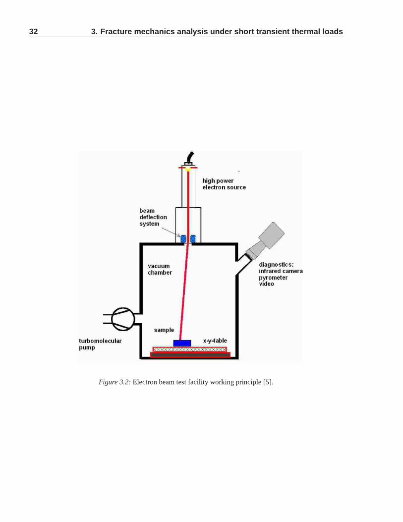
32 3. Fracture mechanics analysis under short transient the rmal loads
Figure 3.2: Electron beam test facility working principle [5].
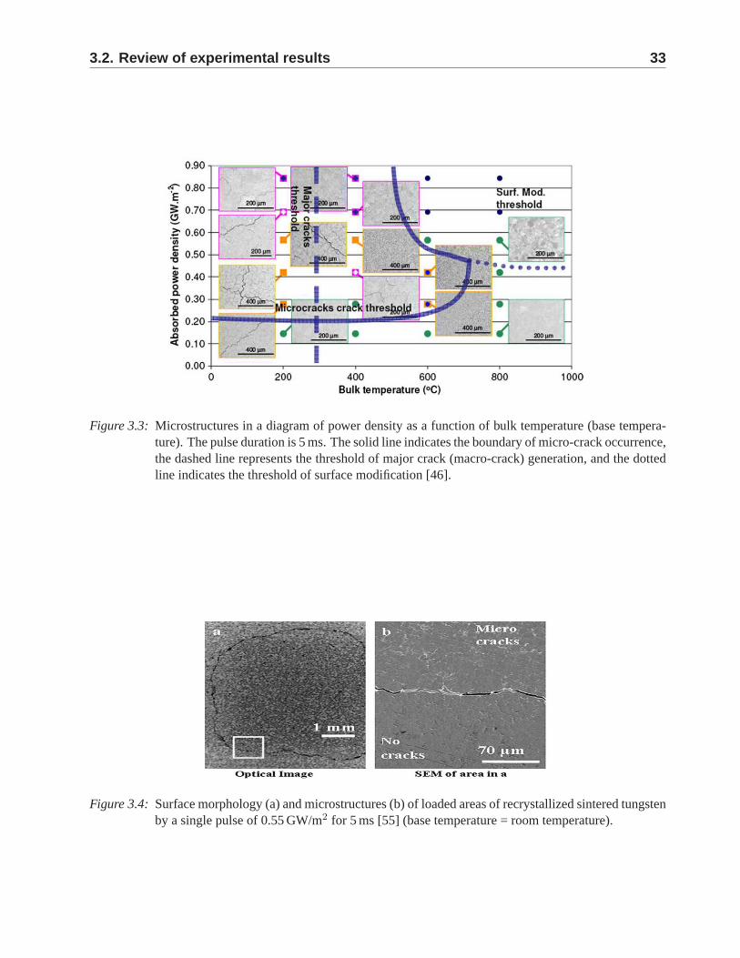
3.2. Review of experimental results 33
Figure 3.3: Microstructures in a diagram of power density as a function of bulk temperature (base tempera-ture). The pulse duration is 5 ms. The solid line indicates the boundary of micro-crack occurrence,the dashed line represents the threshold of major crack (macro-crack) generation, and the dottedline indicates the threshold of surface modification [46].
Figure 3.4: Surface morphology (a) and microstructures (b) of loaded areas of recrystallized sintered tungstenby a single pulse of 0.55 GW/m2 for 5 ms [55] (base temperature = room temperature).
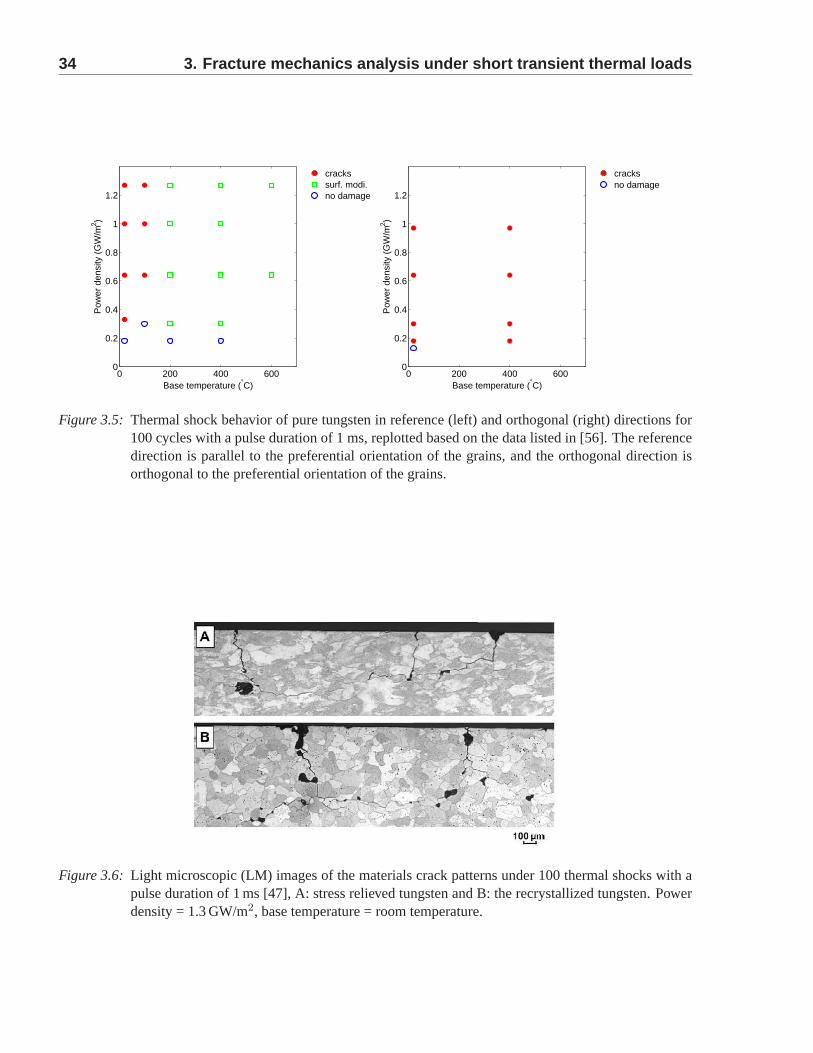
34 3. Fracture mechanics analysis under short transient the rmal loads
0 200 400 6000
0.2
0.4
0.6
0.8
1
1.2
Base temperature (°C)
Pow
er d
ensi
ty (
GW
/m2 )
crackssurf. modi.no damage
0 200 400 6000
0.2
0.4
0.6
0.8
1
1.2
Base temperature (°C)P
ower
den
sity
(G
W/m
2 )
cracksno damage
Figure 3.5: Thermal shock behavior of pure tungsten in reference (left) and orthogonal (right) directions for100 cycles with a pulse duration of 1 ms, replotted based on the data listed in [56]. The referencedirection is parallel to the preferential orientation of the grains, and the orthogonal direction isorthogonal to the preferential orientation of the grains.
Figure 3.6: Light microscopic (LM) images of the materials crack patterns under 100 thermal shocks with apulse duration of 1 ms [47], A: stress relieved tungsten and B: the recrystallized tungsten. Powerdensity = 1.3 GW/m2, base temperature = room temperature.
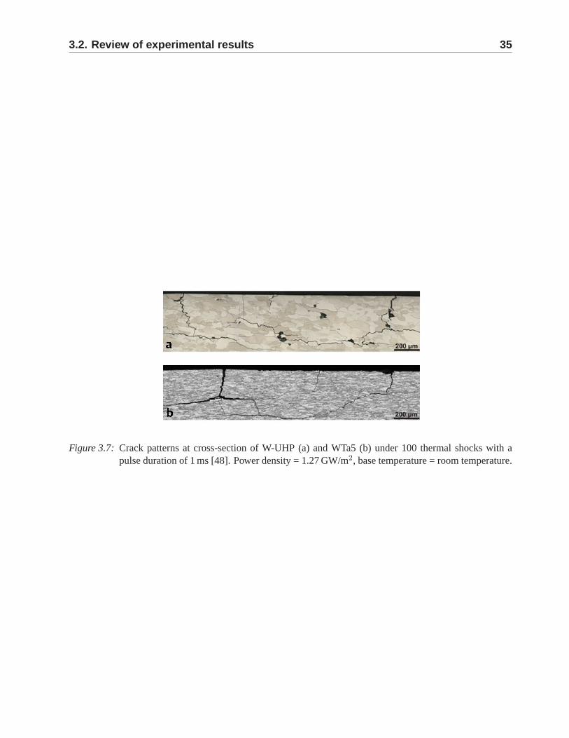
3.2. Review of experimental results 35
Figure 3.7: Crack patterns at cross-section of W-UHP (a) and WTa5 (b) under 100 thermal shocks with apulse duration of 1 ms [48]. Power density = 1.27 GW/m2, base temperature = room temperature.
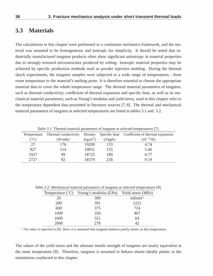
36 3. Fracture mechanics analysis under short transient the rmal loads
3.3 Materials
The calculations in this chapter were performed in a continuum mechanics framework, and the ma-
terial was assumed to be homogeneous and isotropic for simplicity. It should be noted that in-
dustrially manufactured tungsten products often show significant anisotropy in material properties
due to strongly textured microstructure produced by rolling. Isotropic material properties may be
achieved by specific production methods such as powder injection molding. During the thermal
shock experiments, the tungsten samples were subjected to awide range of temperatures - from
room temperature to the material’s melting point. It is therefore essential to choose the appropriate
material data to cover the whole temperature range. The thermal material parameters of tungsten,
such as thermal conductivity, coefficient of thermal expansion and specific heat, as well as its me-
chanical material parameters, such as Young’s modulus and yield stress, used in this chapter refer to
the temperature dependent data presented in literature sources [7, 8]. The thermal and mechanical
material parameters of tungsten at selected temperatures are listed in tables 3.1 and 3.2.
Table 3.1: Thermal material parameters of tungsten at selected temperatures [7].
Temperature Thermal conductivity Density Specific heat Coefficient of thermal expansion(◦C) (W/mK) (kg/m3) (J/kgK) (10−6/K)27 176 19299 133 4.74927 114 19051 155 5.061927 99 18725 180 6.772727 92 18379 218 9.19
Table 3.2: Mechanical material parameters of tungsten at selected temperatures [8].
Temperature (◦C) Young’s modulus (GPa) Yield stress (MPa)20 399 infinitea
200 391 1221600 375 7241000 356 4671600 321 642000 278 42
a No value is reported in [8]. Here, it is assumed that tungstenbehaves purely elastic at this temperature.
The values of the yield stress and the ultimate tensile strength of tungsten are nearly equivalent at
the same temperature [8]. Therefore, tungsten is assumed tobehave elastic-ideally plastic in the
simulations conducted in this chapter.
3.4. Simplified analytical solution 37
3.4 Simplified analytical solution
Numerical methods, such as the finite element method, are widely used in many engineering fields
to capture the complex geometrical and loading conditions.However, an analytical solution can pro-
vide a deeper understanding of the key physical features - and under certain conditions, the analytical
approach can even provide quantitative predictions. In this part, a simplified analytical solution is
derived to estimate the temperature, strain and stress responses of tungsten to homogeneous thermal
loadings.
3.4.1 Temperature calculation
By means of fast scanning of the sample surface with the electron beam, an almost homogeneous
ELM-like transient thermal loading was achieved at the top surface of the tungsten samples [47].
Due to the homogeneity of the thermal loading, the heat conduction in the central part of the loading
area can be assumed to occur only in depth direction.
The energy input induced by the ELMs is much larger than the energy loss due to radiation. When the
thermal loading stops, the decrease of temperature in the surface layer of the tungsten is dominated
by heat conduction rather than thermal radiation at the surface. As a result, the radiation effect can
be neglected in the temperature calculation.
In thermal shock experiments, the thermal penetration depth, beyond which the temperature of the
solid is not affected by the surface temperature, can be calculated as follows [57],
dpen =
√
8k
ρct, (3.1)
wheredpen is the thermal penetration depth,k is the thermal conductivity,ρ is the density,c is the
specific heat, andt denotes time.
Calculations based on the thermal simulations using FEM showed that the surface temperature
dropped below DBTT for typical loading conditions within 5 ms, which indicates that if the tem-
perature at the bottom of the sample is not affected by the surface temperature within 5 ms, the
cooling devices do not play an important role for the temperature evolution at the surface. Substitut-
ing the thermal properties listed in table 3.1 into equation(3.1),dpen at t = 5 ms is smaller than the
sample thickness (5 mm). Based on this result, the heat transfer between the bottom of the sample
and the cooling device can be neglected in a rough temperature calculation.
Considering the above reasons, the solution of a semi-infinite surface heat transfer problem without
considering the radiation effect can provide a fair estimate of the temperature in the central part of
the loading area in thermal shock experiments at Forschungszentrum Julich. H. S. Carslaw and J. C.
Jaeger [58] gave a solution for the temperature of a semi-infinite solid for a heat flux atx = 0 in a
prescribed time with zero initial temperature as follows:
38 3. Fracture mechanics analysis under short transient the rmal loads
(i) 0< t ≤ th
T − T0 =2q
k{(
κt
π
1
2
)e−x
2
4κt − x
2erfc(
x
2√
κt)}, (3.2)
(ii) t > th
T − T0 =2qκ
1
2
k{t
1
2 ierfc(x
2κ1
2 t1
2
) − (t − th)1
2 ierfc(x
2κ1
2 (t − th)1
2
)}, (3.3)
whereT is temperature,T0 is the initial temperature,q is the heat flux,t is time, th is the heating
time, κ is the thermal diffusivity, which is equal tok/ρc, erfc is the complementary error function
given by
erfc(x) =2√π
∫
∞
xe−t2
dt. (3.4)
The iterated integrals of the complementary error functionare defined by
inerfc(z) =∫
∞
zin−1erfc(ζ)dζ. (3.5)
To verify the analytical results, thermal simulations using the commercial finite element code ABAQUS
were performed. A heat flux load of 1.27 GW/m2 was applied at the top surface for 1 ms. Two ther-
mal simulations were carried out with constant thermal material parameters at room temperature
and temperature dependent thermal material parameters, respectively. The analytical solution was
obtained from equations (3.2) and (3.3). The analytically calculated temperature curve fits very well
with the numerical solution with constant thermal materialparameters, see figure 3.8. Figure 3.9
shows the maximum temperatures at various depths, which differ from the temperatures at the end
of heating. When heating stops, the temperature at the top surface drops immediately, but the tem-
perature in the deeper parts continuously increases shortly after, since the heat conduction into the
material needs some time.
In order to predict more precise temperature profiles, the constant thermal material parameters at an
elevated temperature - which is set to be half of the maximum temperature at the top surface - is
applied in the analytical formula. The analytical temperature prediction using the constant thermal
material parameters at the elevated temperature fits quite well with the thermal simulation based on
the fully temperature dependent thermal material parameters, see figure 3.10.
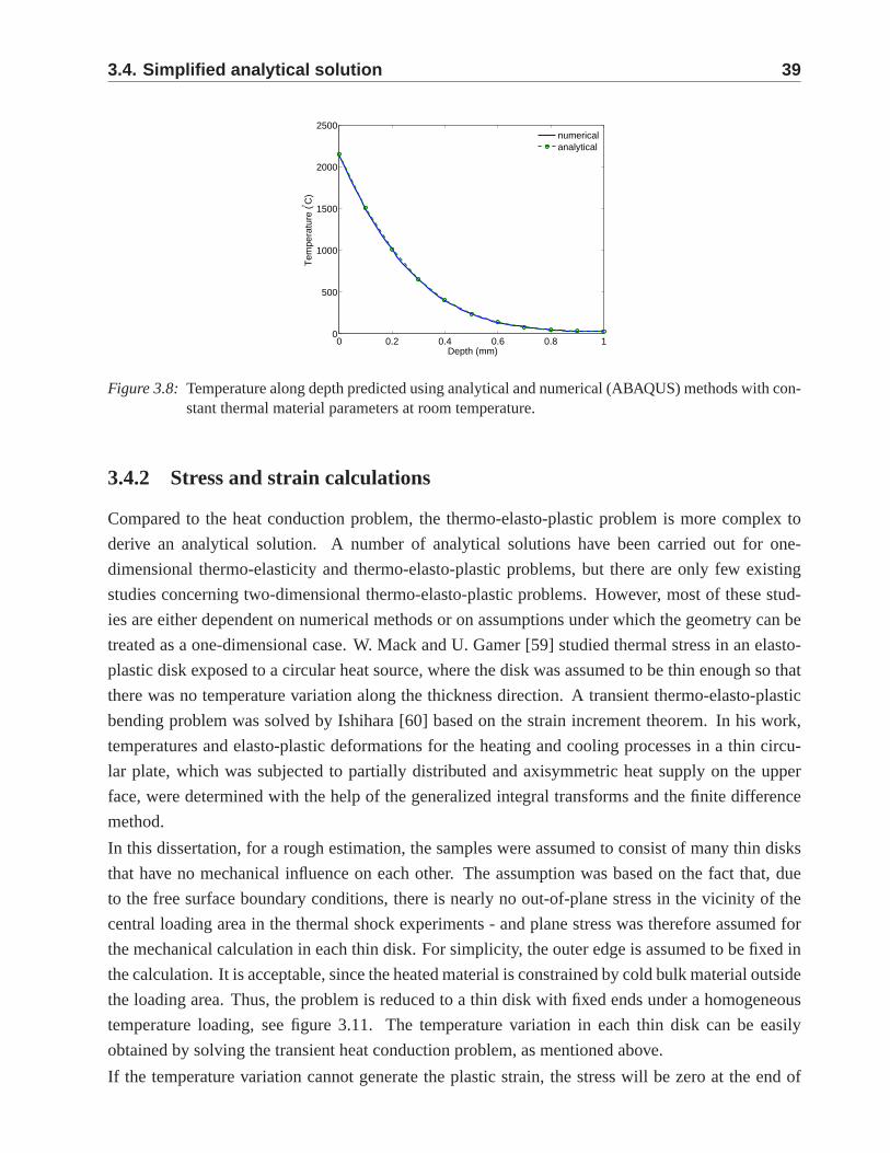
3.4. Simplified analytical solution 39
0 0.2 0.4 0.6 0.8 10
500
1000
1500
2000
2500
Depth (mm)
Tem
pera
ture
(° C)
numericalanalytical
Figure 3.8: Temperature along depth predicted using analytical and numerical (ABAQUS) methods with con-stant thermal material parameters at room temperature.
3.4.2 Stress and strain calculations
Compared to the heat conduction problem, the thermo-elasto-plastic problem is more complex to
derive an analytical solution. A number of analytical solutions have been carried out for one-
dimensional thermo-elasticity and thermo-elasto-plastic problems, but there are only few existing
studies concerning two-dimensional thermo-elasto-plastic problems. However, most of these stud-
ies are either dependent on numerical methods or on assumptions under which the geometry can be
treated as a one-dimensional case. W. Mack and U. Gamer [59] studied thermal stress in an elasto-
plastic disk exposed to a circular heat source, where the disk was assumed to be thin enough so that
there was no temperature variation along the thickness direction. A transient thermo-elasto-plastic
bending problem was solved by Ishihara [60] based on the strain increment theorem. In his work,
temperatures and elasto-plastic deformations for the heating and cooling processes in a thin circu-
lar plate, which was subjected to partially distributed andaxisymmetric heat supply on the upper
face, were determined with the help of the generalized integral transforms and the finite difference
method.
In this dissertation, for a rough estimation, the samples were assumed to consist of many thin disks
that have no mechanical influence on each other. The assumption was based on the fact that, due
to the free surface boundary conditions, there is nearly no out-of-plane stress in the vicinity of the
central loading area in the thermal shock experiments - and plane stress was therefore assumed for
the mechanical calculation in each thin disk. For simplicity, the outer edge is assumed to be fixed in
the calculation. It is acceptable, since the heated material is constrained by cold bulk material outside
the loading area. Thus, the problem is reduced to a thin disk with fixed ends under a homogeneous
temperature loading, see figure 3.11. The temperature variation in each thin disk can be easily
obtained by solving the transient heat conduction problem,as mentioned above.
If the temperature variation cannot generate the plastic strain, the stress will be zero at the end of
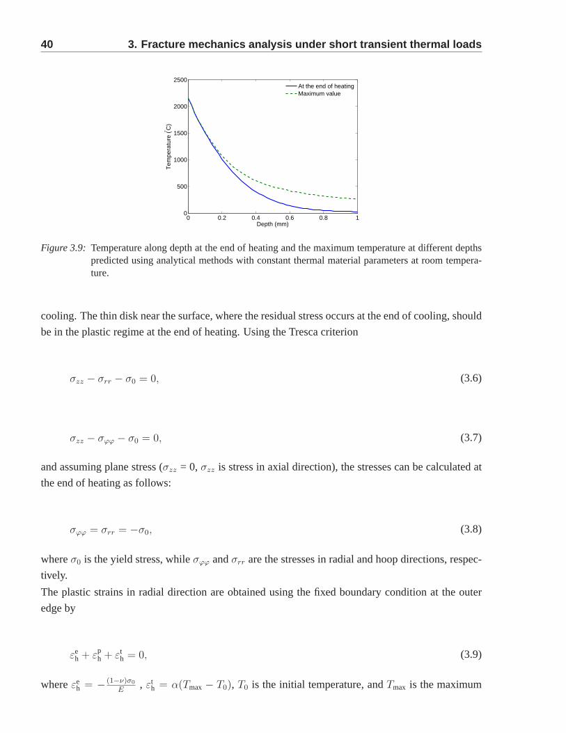
40 3. Fracture mechanics analysis under short transient the rmal loads
0 0.2 0.4 0.6 0.8 10
500
1000
1500
2000
2500
Depth (mm)
Tem
pera
ture
(° C)
At the end of heatingMaximum value
Figure 3.9: Temperature along depth at the end of heating and the maximum temperature at different depthspredicted using analytical methods with constant thermal material parameters at room tempera-ture.
cooling. The thin disk near the surface, where the residual stress occurs at the end of cooling, should
be in the plastic regime at the end of heating. Using the Tresca criterion
σzz − σrr − σ0 = 0, (3.6)
σzz − σϕϕ − σ0 = 0, (3.7)
and assuming plane stress (σzz = 0, σzz is stress in axial direction), the stresses can be calculated at
the end of heating as follows:
σϕϕ = σrr = −σ0, (3.8)
whereσ0 is the yield stress, whileσϕϕ andσrr are the stresses in radial and hoop directions, respec-
tively.
The plastic strains in radial direction are obtained using the fixed boundary condition at the outer
edge by
εeh + εp
h + εth = 0, (3.9)
whereεeh = − (1−ν)σ0
E, εt
h = α(Tmax − T0), T0 is the initial temperature, andTmax is the maximum
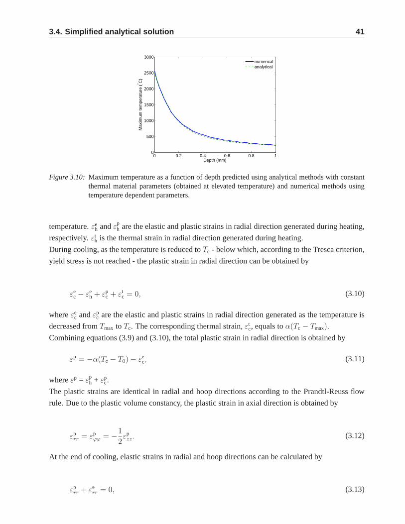
3.4. Simplified analytical solution 41
0 0.2 0.4 0.6 0.8 10
500
1000
1500
2000
2500
3000
Depth (mm)
Max
imum
tem
pera
ture
(° C
)
numericalanalytical
Figure 3.10: Maximum temperature as a function of depth predicted using analytical methodswith constantthermal material parameters (obtained at elevated temperature) and numerical methods usingtemperature dependent parameters.
temperature.εeh andεp
h are the elastic and plastic strains in radial direction generated during heating,
respectively.εth is the thermal strain in radial direction generated during heating.
During cooling, as the temperature is reduced toTc - below which, according to the Tresca criterion,
yield stress is not reached - the plastic strain in radial direction can be obtained by
εec − εe
h + εpc + εt
c = 0, (3.10)
whereεec andεp
c are the elastic and plastic strains in radial direction generated as the temperature is
decreased fromTmax to Tc. The corresponding thermal strain,εtc, equals toα(Tc − Tmax).
Combining equations (3.9) and (3.10), the total plastic strain in radial direction is obtained by
εp = −α(Tc − T0) − εec, (3.11)
whereεp = εph + εp
c.
The plastic strains are identical in radial and hoop directions according to the Prandtl-Reuss flow
rule. Due to the plastic volume constancy, the plastic strain in axial direction is obtained by
εprr = εp
ϕϕ = −1
2εp
zz. (3.12)
At the end of cooling, elastic strains in radial and hoop directions can be calculated by
εprr + εe
rr = 0, (3.13)
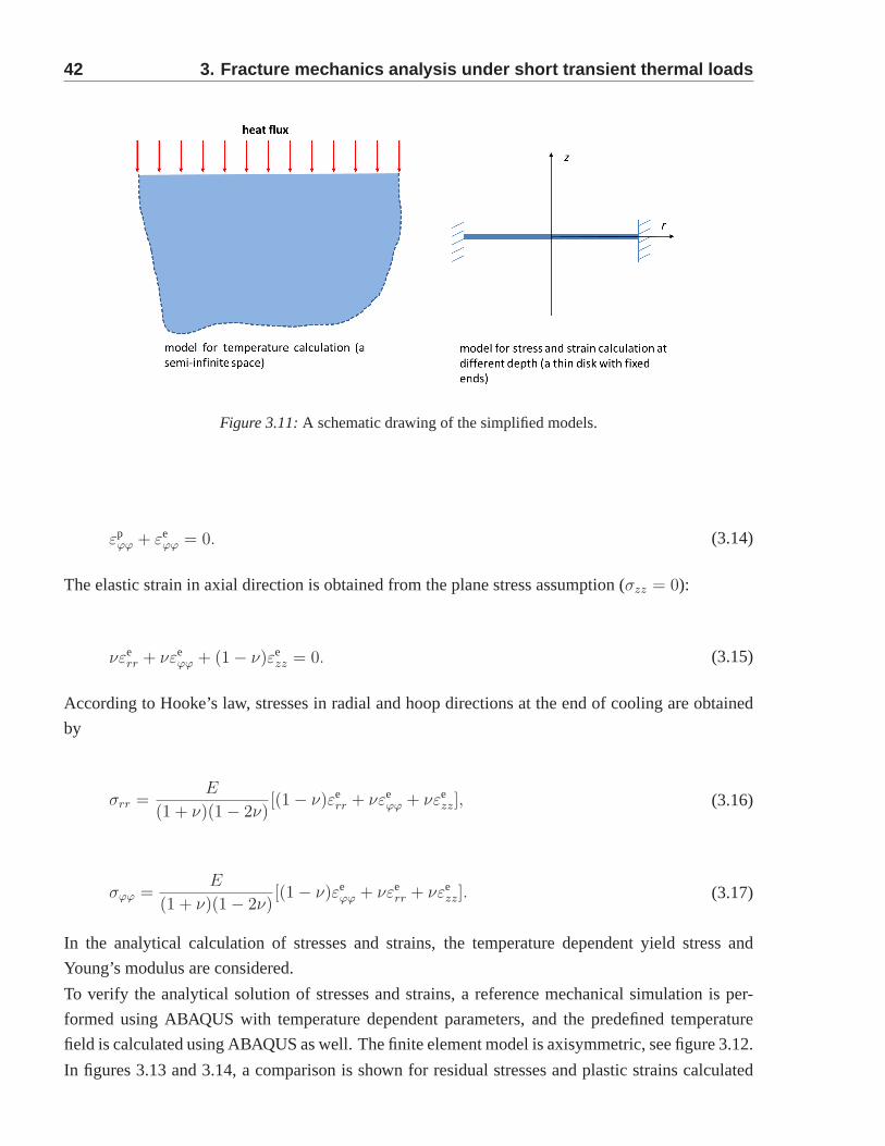
42 3. Fracture mechanics analysis under short transient the rmal loads
Figure 3.11: A schematic drawing of the simplified models.
εpϕϕ + εe
ϕϕ = 0. (3.14)
The elastic strain in axial direction is obtained from the plane stress assumption (σzz = 0):
νεerr + νεe
ϕϕ + (1 − ν)εezz = 0. (3.15)
According to Hooke’s law, stresses in radial and hoop directions at the end of cooling are obtained
by
σrr =E
(1 + ν)(1 − 2ν)[(1 − ν)εe
rr + νεeϕϕ + νεe
zz], (3.16)
σϕϕ =E
(1 + ν)(1 − 2ν)[(1 − ν)εe
ϕϕ + νεerr + νεe
zz]. (3.17)
In the analytical calculation of stresses and strains, the temperature dependent yield stress and
Young’s modulus are considered.
To verify the analytical solution of stresses and strains, areference mechanical simulation is per-
formed using ABAQUS with temperature dependent parameters, and the predefined temperature
field is calculated using ABAQUS as well. The finite element model is axisymmetric, see figure 3.12.
In figures 3.13 and 3.14, a comparison is shown for residual stresses and plastic strains calculated
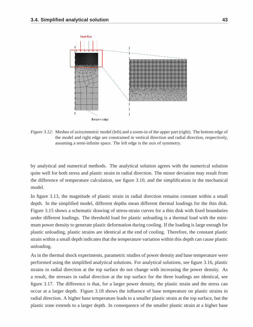
3.4. Simplified analytical solution 43
Figure 3.12: Meshes of axisymmetric model (left) and a zoom-in of the upper part (right).The bottom edge ofthe model and right edge are constrained in vertical direction and radial direction, respectively,assuming a semi-infinite space. The left edge is the axis of symmetry.
by analytical and numerical methods. The analytical solution agrees with the numerical solution
quite well for both stress and plastic strain in radial direction. The minor deviation may result from
the difference of temperature calculation, see figure 3.10,and the simplification in the mechanical
model.
In figure 3.13, the magnitude of plastic strain in radial direction remains constant within a small
depth. In the simplified model, different depths mean different thermal loadings for the thin disk.
Figure 3.15 shows a schematic drawing of stress-strain curves for a thin disk with fixed boundaries
under different loadings. The threshold load for plastic unloading is a thermal load with the mini-
mum power density to generate plastic deformation during cooling. If the loading is large enough for
plastic unloading, plastic strains are identical at the endof cooling. Therefore, the constant plastic
strain within a small depth indicates that the temperature variation within this depth can cause plastic
unloading.
As in the thermal shock experiments, parametric studies of power density and base temperature were
performed using the simplified analytical solutions. For analytical solutions, see figure 3.16, plastic
strains in radial direction at the top surface do not change with increasing the power density. As
a result, the stresses in radial direction at the top surfacefor the three loadings are identical, see
figure 3.17. The difference is that, for a larger power density, the plastic strain and the stress can
occur at a larger depth. Figure 3.18 shows the influence of base temperature on plastic strains in
radial direction. A higher base temperature leads to a smaller plastic strain at the top surface, but the
plastic zone extends to a larger depth. In consequence of thesmaller plastic strain at a higher base
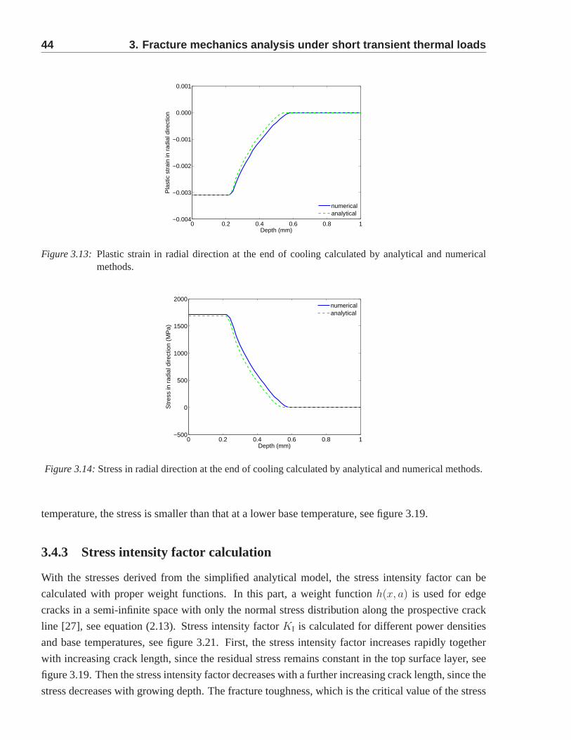
44 3. Fracture mechanics analysis under short transient the rmal loads
0 0.2 0.4 0.6 0.8 1−0.004
−0.003
−0.002
−0.001
0.000
0.001
Depth (mm)
Pla
stic
str
ain
in r
adia
l dire
ctio
n
numericalanalytical
Figure 3.13: Plastic strain in radial direction at the end of cooling calculated by analytical and numericalmethods.
0 0.2 0.4 0.6 0.8 1−500
0
500
1000
1500
2000
Depth (mm)
Str
ess
in r
adia
l dire
ctio
n (M
Pa)
numericalanalytical
Figure 3.14: Stress in radial direction at the end of cooling calculated by analytical and numerical methods.
temperature, the stress is smaller than that at a lower base temperature, see figure 3.19.
3.4.3 Stress intensity factor calculation
With the stresses derived from the simplified analytical model, the stress intensity factor can be
calculated with proper weight functions. In this part, a weight functionh(x, a) is used for edge
cracks in a semi-infinite space with only the normal stress distribution along the prospective crack
line [27], see equation (2.13). Stress intensity factorKI is calculated for different power densities
and base temperatures, see figure 3.21. First, the stress intensity factor increases rapidly together
with increasing crack length, since the residual stress remains constant in the top surface layer, see
figure 3.19. Then the stress intensity factor decreases witha further increasing crack length, since the
stress decreases with growing depth. The fracture toughness, which is the critical value of the stress
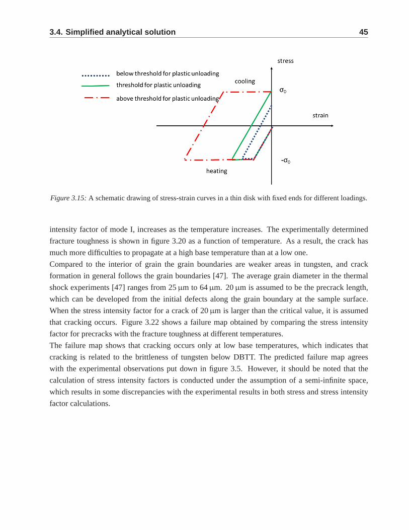
3.4. Simplified analytical solution 45
Figure 3.15: A schematic drawing of stress-strain curves in a thin disk with fixed ends fordifferent loadings.
intensity factor of mode I, increases as the temperature increases. The experimentally determined
fracture toughness is shown in figure 3.20 as a function of temperature. As a result, the crack has
much more difficulties to propagate at a high base temperature than at a low one.
Compared to the interior of grain the grain boundaries are weaker areas in tungsten, and crack
formation in general follows the grain boundaries [47]. Theaverage grain diameter in the thermal
shock experiments [47] ranges from 25µm to 64µm. 20µm is assumed to be the precrack length,
which can be developed from the initial defects along the grain boundary at the sample surface.
When the stress intensity factor for a crack of 20µm is larger than the critical value, it is assumed
that cracking occurs. Figure 3.22 shows a failure map obtained by comparing the stress intensity
factor for precracks with the fracture toughness at different temperatures.
The failure map shows that cracking occurs only at low base temperatures, which indicates that
cracking is related to the brittleness of tungsten below DBTT. The predicted failure map agrees
with the experimental observations put down in figure 3.5. However, it should be noted that the
calculation of stress intensity factors is conducted underthe assumption of a semi-infinite space,
which results in some discrepancies with the experimental results in both stress and stress intensity
factor calculations.
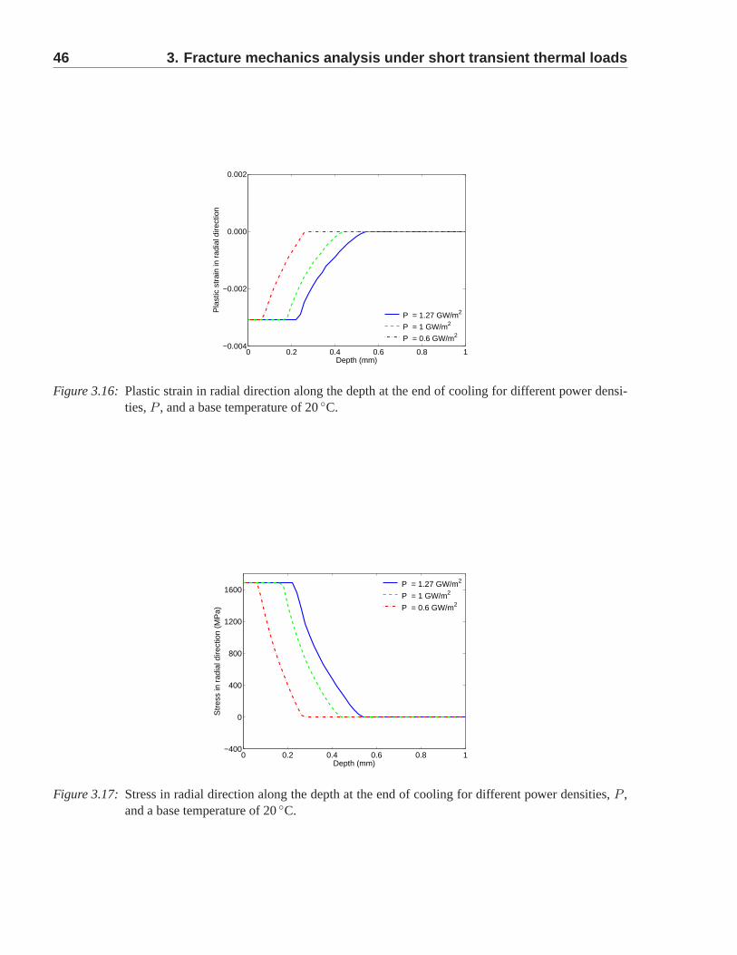
46 3. Fracture mechanics analysis under short transient the rmal loads
0 0.2 0.4 0.6 0.8 1−0.004
−0.002
0.000
0.002
Depth (mm)
Pla
stic
str
ain
in r
adia
l dire
ctio
n
P = 1.27 GW/m2
P = 1 GW/m2
P = 0.6 GW/m2
Figure 3.16: Plastic strain in radial direction along the depth at the end of cooling for different power densi-ties,P , and a base temperature of 20◦C.
0 0.2 0.4 0.6 0.8 1−400
0
400
800
1200
1600
Depth (mm)
Str
ess
in r
adia
l dire
ctio
n (M
Pa)
P = 1.27 GW/m2
P = 1 GW/m2
P = 0.6 GW/m2
Figure 3.17: Stress in radial direction along the depth at the end of cooling for different power densities,P ,and a base temperature of 20◦C.
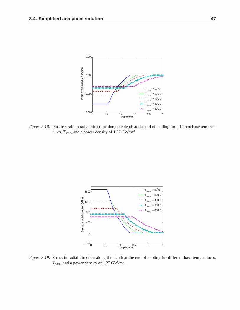
3.4. Simplified analytical solution 47
0 0.2 0.4 0.6 0.8 1−0.004
−0.002
0.000
0.002
Depth (mm)
Pla
stic
str
ain
in r
adia
l dire
ctio
n
T base
= 20°C
T base
= 200°C
T base
= 400°C
T base
= 600°C
T base
= 800°C
Figure 3.18: Plastic strain in radial direction along the depth at the end of cooling for different base tempera-tures,Tbase, and a power density of 1.27 GW/m2.
0 0.2 0.4 0.6 0.8 1−400
0
400
800
1200
1600
Depth (mm)
Str
ess
in r
adia
l dire
ctio
n (M
Pa)
T base
= 20°C
T base
= 200°C
T base
= 400°C
T base
= 600°C
T base
= 800°C
Figure 3.19: Stress in radial direction along the depth at the end of cooling for different base temperatures,Tbase, and a power density of 1.27 GW/m2.
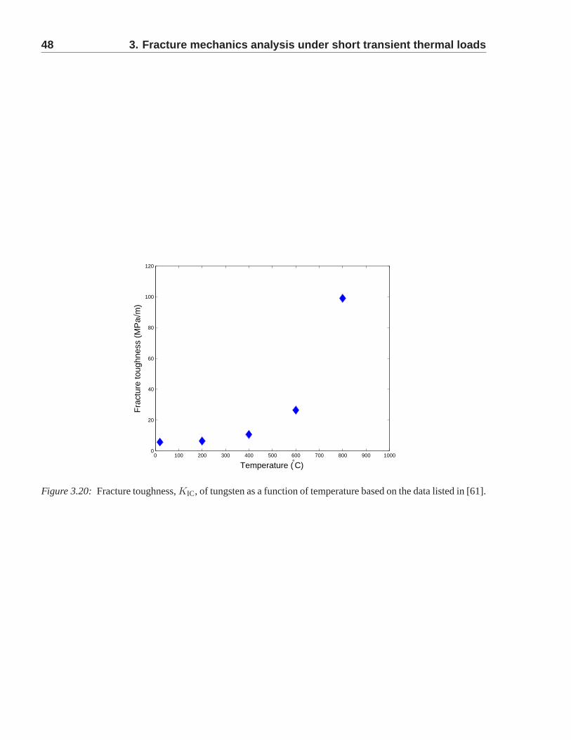
48 3. Fracture mechanics analysis under short transient the rmal loads
0 100 200 300 400 500 600 700 800 900 10000
20
40
60
80
100
120
Temperature (°C)
Fra
ctur
e to
ughn
ess
(MP
a√m
)
Figure 3.20: Fracture toughness,KIC, of tungsten as a function of temperature based on the data listed in [61].
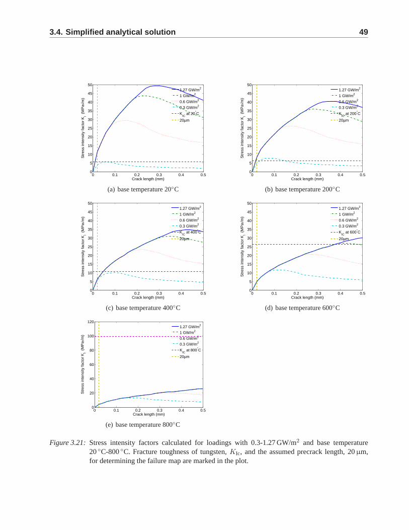
3.4. Simplified analytical solution 49
0 0.1 0.2 0.3 0.4 0.50
5
10
15
20
25
30
35
40
45
50
Crack length (mm)
Str
ess
inte
nsity
fact
or K
I (M
Pa√
m)
1.27 GW/m2
1 GW/m2
0.6 GW/m2
0.3 GW/m2
KIC
at 20°C
20µm
(a) base temperature 20◦C
0 0.1 0.2 0.3 0.4 0.50
5
10
15
20
25
30
35
40
45
50
Crack length (mm)
Str
ess
inte
nsity
fact
or K
I (M
Pa√
m)
1.27 GW/m2
1 GW/m2
0.6 GW/m2
0.3 GW/m2
KIC
at 200°C
20µm
(b) base temperature 200◦C
0 0.1 0.2 0.3 0.4 0.50
5
10
15
20
25
30
35
40
45
50
Crack length (mm)
Str
ess
inte
nsity
fact
or K
I (M
Pa√
m)
1.27 GW/m2
1 GW/m2
0.6 GW/m2
0.3 GW/m2
KIC
at 400°C
20µm
(c) base temperature 400◦C
0 0.1 0.2 0.3 0.4 0.50
5
10
15
20
25
30
35
40
45
50
Crack length (mm)
Str
ess
inte
nsity
fact
or K
I (M
Pa√
m)
1.27 GW/m2
1 GW/m2
0.6 GW/m2
0.3 GW/m2
KIC
at 600°C
20µm
(d) base temperature 600◦C
0 0.1 0.2 0.3 0.4 0.50
20
40
60
80
100
120
Crack length (mm)
Str
ess
inte
nsity
fact
or K
I (M
Pa√
m)
1.27 GW/m2
1 GW/m2
0.6 GW/m2
0.3 GW/m2
KIC
at 800°C
20µm
(e) base temperature 800◦C
Figure 3.21: Stress intensity factors calculated for loadings with 0.3-1.27 GW/m2 and base temperature20◦C-800◦C. Fracture toughness of tungsten,KIc, and the assumed precrack length, 20µm,for determining the failure map are marked in the plot.
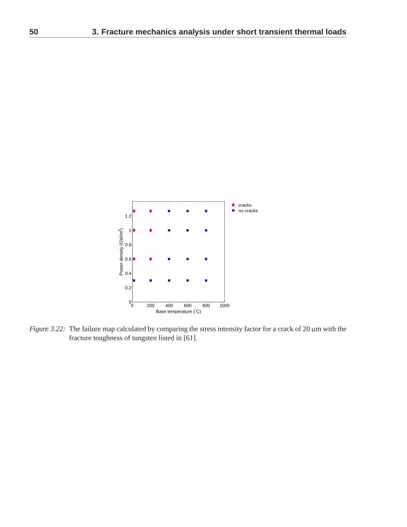
50 3. Fracture mechanics analysis under short transient the rmal loads
0 200 400 600 800 10000
0.2
0.4
0.6
0.8
1
1.2
Base temperature (°C)
Pow
er d
ensi
ty (
GW
/m2 )
cracksno cracks
Figure 3.22: The failure map calculated by comparing the stress intensity factor for a crack of 20µm with thefracture toughness of tungsten listed in [61].
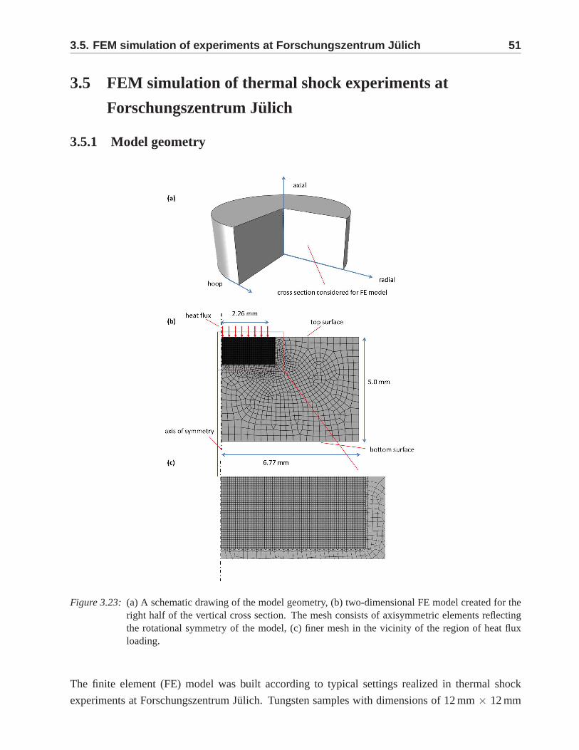
3.5. FEM simulation of experiments at Forschungszentrum Ju lich 51
3.5 FEM simulation of thermal shock experiments at
Forschungszentrum Julich
3.5.1 Model geometry
Figure 3.23: (a) A schematic drawing of the model geometry, (b) two-dimensional FE modelcreated for theright half of the vertical cross section. The mesh consists of axisymmetric elements reflectingthe rotational symmetry of the model, (c) finer mesh in the vicinity of the region of heat fluxloading.
The finite element (FE) model was built according to typical settings realized in thermal shock
experiments at Forschungszentrum Julich. Tungsten samples with dimensions of 12 mm× 12 mm
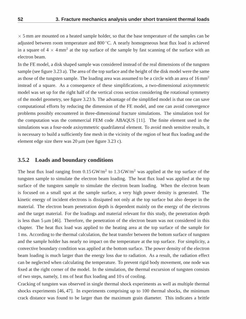
52 3. Fracture mechanics analysis under short transient the rmal loads
× 5 mm are mounted on a heated sample holder, so that the base temperature of the samples can be
adjusted between room temperature and 800◦C. A nearly homogeneous heat flux load is achieved
in a square of 4× 4 mm2 at the top surface of the sample by fast scanning of the surface with an
electron beam.
In the FE model, a disk shaped sample was considered instead of the real dimensions of the tungsten
sample (see figure 3.23 a). The area of the top surface and the height of the disk model were the same
as those of the tungsten sample. The loading area was assumedto be a circle with an area of 16 mm2
instead of a square. As a consequence of these simplifications, a two-dimensional axisymmetric
model was set up for the right half of the vertical cross section considering the rotational symmetry
of the model geometry, see figure 3.23 b. The advantage of the simplified model is that one can save
computational efforts by reducing the dimension of the FE model, and one can avoid convergence
problems possibly encountered in three-dimensional fracture simulations. The simulation tool for
the computation was the commercial FEM code ABAQUS [11]. Thefinite element used in the
simulations was a four-node axisymmetric quadrilateral element. To avoid mesh sensitive results, it
is necessary to build a sufficiently fine mesh in the vicinity of the region of heat flux loading and the
element edge size there was 20µm (see figure 3.23 c).
3.5.2 Loads and boundary conditions
The heat flux load ranging from 0.15 GW/m2 to 1.3 GW/m2 was applied at the top surface of the
tungsten sample to simulate the electron beam loading. The heat flux load was applied at the top
surface of the tungsten sample to simulate the electron beamloading. When the electron beam
is focused on a small spot at the sample surface, a very high power density is generated. The
kinetic energy of incident electrons is dissipated not onlyat the top surface but also deeper in the
material. The electron beam penetration depth is dependentmainly on the energy of the electrons
and the target material. For the loadings and material relevant for this study, the penetration depth
is less than 5µm [46]. Therefore, the penetration of the electron beam was not considered in this
chapter. The heat flux load was applied to the heating area at the top surface of the sample for
1 ms. According to the thermal calculation, the heat transfer between the bottom surface of tungsten
and the sample holder has nearly no impact on the temperatureat the top surface. For simplicity, a
convective boundary condition was applied at the bottom surface. The power density of the electron
beam loading is much larger than the energy loss due to radiation. As a result, the radiation effect
can be neglected when calculating the temperature. To prevent rigid body movement, one node was
fixed at the right corner of the model. In the simulation, the thermal excursion of tungsten consists
of two steps, namely, 1 ms of heat flux loading and 10 s of cooling.
Cracking of tungsten was observed in single thermal shock experiments as well as multiple thermal
shocks experiments [46, 47]. In experiments comprising up to 100 thermal shocks, the minimum
crack distance was found to be larger than the maximum grain diameter. This indicates a brittle
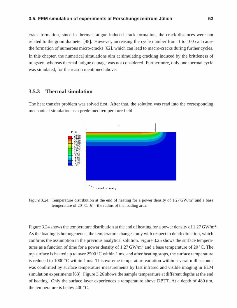
3.5. FEM simulation of experiments at Forschungszentrum Ju lich 53
crack formation, since in thermal fatigue induced crack formation, the crack distances were not
related to the grain diameter [48]. However, increasing thecycle number from 1 to 100 can cause
the formation of numerous micro-cracks [62], which can leadto macro-cracks during further cycles.
In this chapter, the numerical simulations aim at simulating cracking induced by the brittleness of
tungsten, whereas thermal fatigue damage was not considered. Furthermore, only one thermal cycle
was simulated, for the reason mentioned above.
3.5.3 Thermal simulation
The heat transfer problem was solved first. After that, the solution was read into the corresponding
mechanical simulation as a predefined temperature field.
Figure 3.24: Temperature distribution at the end of heating for a power density of 1.27 GW/m2 and a basetemperature of 20◦C. R = the radius of the loading area.
Figure 3.24 shows the temperature distribution at the end ofheating for a power density of 1.27 GW/m2.
As the loading is homogeneous, the temperature changes onlywith respect to depth direction, which
confirms the assumption in the previous analytical solution. Figure 3.25 shows the surface tempera-
tures as a function of time for a power density of 1.27 GW/m2 and a base temperature of 20◦C. The
top surface is heated up to over 2500◦C within 1 ms, and after heating stops, the surface temperature
is reduced to 1000◦C within 1 ms. This extreme temperature variation within several milliseconds
was confirmed by surface temperature measurements by fast infrared and visible imaging in ELM
simulation experiments [63]. Figure 3.26 shows the sample temperature at different depths at the end
of heating. Only the surface layer experiences a temperature above DBTT. At a depth of 480µm,
the temperature is below 400◦C.
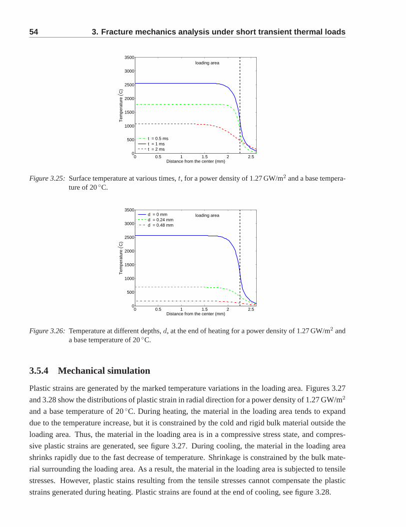
54 3. Fracture mechanics analysis under short transient the rmal loads
0 0.5 1 1.5 2 2.50
500
1000
1500
2000
2500
3000
3500loading area
Distance from the center (mm)
Tem
pera
ture
(° C)
t = 0.5 ms t = 1 ms t = 2 ms
Figure 3.25: Surface temperature at various times,t, for a power density of 1.27 GW/m2 and a base tempera-ture of 20◦C.
0 0.5 1 1.5 2 2.50
500
1000
1500
2000
2500
3000
3500loading area
Distance from the center (mm)
Tem
pera
ture
(° C)
d = 0 mm d = 0.24 mm d = 0.48 mm
Figure 3.26: Temperature at different depths,d, at the end of heating for a power density of 1.27 GW/m2 anda base temperature of 20◦C.
3.5.4 Mechanical simulation
Plastic strains are generated by the marked temperature variations in the loading area. Figures 3.27
and 3.28 show the distributions of plastic strain in radial direction for a power density of 1.27 GW/m2
and a base temperature of 20◦C. During heating, the material in the loading area tends to expand
due to the temperature increase, but it is constrained by thecold and rigid bulk material outside the
loading area. Thus, the material in the loading area is in a compressive stress state, and compres-
sive plastic strains are generated, see figure 3.27. During cooling, the material in the loading area
shrinks rapidly due to the fast decrease of temperature. Shrinkage is constrained by the bulk mate-
rial surrounding the loading area. As a result, the materialin the loading area is subjected to tensile
stresses. However, plastic stains resulting from the tensile stresses cannot compensate the plastic
strains generated during heating. Plastic strains are found at the end of cooling, see figure 3.28.
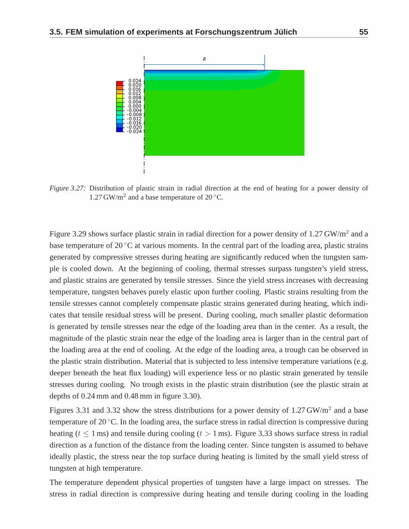
3.5. FEM simulation of experiments at Forschungszentrum Ju lich 55
Figure 3.27: Distribution of plastic strain in radial direction at the end of heating for a power density of1.27 GW/m2 and a base temperature of 20◦C.
Figure 3.29 shows surface plastic strain in radial direction for a power density of 1.27 GW/m2 and a
base temperature of 20◦C at various moments. In the central part of the loading area,plastic strains
generated by compressive stresses during heating are significantly reduced when the tungsten sam-
ple is cooled down. At the beginning of cooling, thermal stresses surpass tungsten’s yield stress,
and plastic strains are generated by tensile stresses. Since the yield stress increases with decreasing
temperature, tungsten behaves purely elastic upon furthercooling. Plastic strains resulting from the
tensile stresses cannot completely compensate plastic strains generated during heating, which indi-
cates that tensile residual stress will be present. During cooling, much smaller plastic deformation
is generated by tensile stresses near the edge of the loadingarea than in the center. As a result, the
magnitude of the plastic strain near the edge of the loading area is larger than in the central part of
the loading area at the end of cooling. At the edge of the loading area, a trough can be observed in
the plastic strain distribution. Material that is subjected to less intensive temperature variations (e.g.
deeper beneath the heat flux loading) will experience less orno plastic strain generated by tensile
stresses during cooling. No trough exists in the plastic strain distribution (see the plastic strain at
depths of 0.24 mm and 0.48 mm in figure 3.30).
Figures 3.31 and 3.32 show the stress distributions for a power density of 1.27 GW/m2 and a base
temperature of 20◦C. In the loading area, the surface stress in radial directionis compressive during
heating (t ≤ 1 ms) and tensile during cooling (t > 1 ms). Figure 3.33 shows surface stress in radial
direction as a function of the distance from the loading center. Since tungsten is assumed to behave
ideally plastic, the stress near the top surface during heating is limited by the small yield stress of
tungsten at high temperature.
The temperature dependent physical properties of tungstenhave a large impact on stresses. The
stress in radial direction is compressive during heating and tensile during cooling in the loading
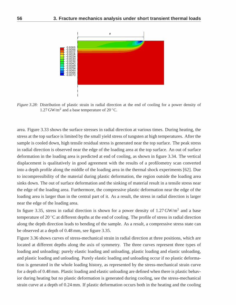
56 3. Fracture mechanics analysis under short transient the rmal loads
Figure 3.28: Distribution of plastic strain in radial direction at the end of cooling for a power density of1.27 GW/m2 and a base temperature of 20◦C.
area. Figure 3.33 shows the surface stresses in radial direction at various times. During heating, the
stress at the top surface is limited by the small yield stressof tungsten at high temperatures. After the
sample is cooled down, high tensile residual stress is generated near the top surface. The peak stress
in radial direction is observed near the edge of the loading area at the top surface. An out of surface
deformation in the loading area is predicted at end of cooling, as shown in figure 3.34. The vertical
displacement is qualitatively in good agreement with the results of a profilometry scan converted
into a depth profile along the middle of the loading area in thethermal shock experiments [62]. Due
to incompressibility of the material during plastic deformation, the region outside the loading area
sinks down. The out of surface deformation and the sinking ofmaterial result in a tensile stress near
the edge of the loading area. Furthermore, the compressive plastic deformation near the edge of the
loading area is larger than in the central part of it. As a result, the stress in radial direction is larger
near the edge of the loading area.
In figure 3.35, stress in radial direction is shown for a powerdensity of 1.27 GW/m2 and a base
temperature of 20◦C at different depths at the end of cooling. The profile of stress in radial direction
along the depth direction leads to bending of the sample. As aresult, a compressive stress state can
be observed at a depth of 0.48 mm, see figure 3.35.
Figure 3.36 shows curves of stress-mechanical strain in radial direction at three positions, which are
located at different depths along the axis of symmetry. The three curves represent three types of
loading and unloading: purely elastic loading and unloading, plastic loading and elastic unloading,
and plastic loading and unloading. Purely elastic loading and unloading occur if no plastic deforma-
tion is generated in the whole loading history, as represented by the stress-mechanical strain curve
for a depth of 0.48 mm. Plastic loading and elastic unloadingare defined when there is plastic behav-
ior during heating but no plastic deformation is generated during cooling, see the stress-mechanical
strain curve at a depth of 0.24 mm. If plastic deformation occurs both in the heating and the cooling
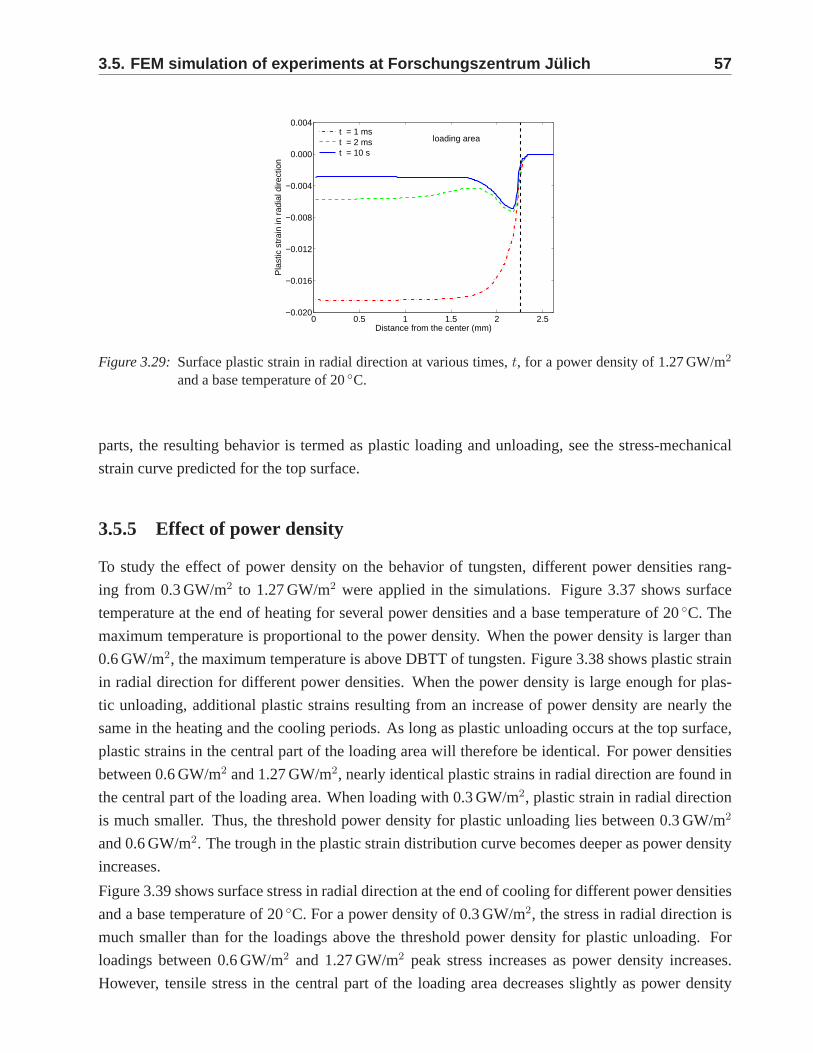
3.5. FEM simulation of experiments at Forschungszentrum Ju lich 57
0 0.5 1 1.5 2 2.5−0.020
−0.016
−0.012
−0.008
−0.004
0.000
0.004
loading area
Distance from the center (mm)
Pla
stic
str
ain
in r
adia
l dire
ctio
n
t = 1 ms t = 2 ms t = 10 s
Figure 3.29: Surface plastic strain in radial direction at various times,t, for a power density of 1.27 GW/m2
and a base temperature of 20◦C.
parts, the resulting behavior is termed as plastic loading and unloading, see the stress-mechanical
strain curve predicted for the top surface.
3.5.5 Effect of power density
To study the effect of power density on the behavior of tungsten, different power densities rang-
ing from 0.3 GW/m2 to 1.27 GW/m2 were applied in the simulations. Figure 3.37 shows surface
temperature at the end of heating for several power densities and a base temperature of 20◦C. The
maximum temperature is proportional to the power density. When the power density is larger than
0.6 GW/m2, the maximum temperature is above DBTT of tungsten. Figure 3.38 shows plastic strain
in radial direction for different power densities. When the power density is large enough for plas-
tic unloading, additional plastic strains resulting from an increase of power density are nearly the
same in the heating and the cooling periods. As long as plastic unloading occurs at the top surface,
plastic strains in the central part of the loading area will therefore be identical. For power densities
between 0.6 GW/m2 and 1.27 GW/m2, nearly identical plastic strains in radial direction are found in
the central part of the loading area. When loading with 0.3 GW/m2, plastic strain in radial direction
is much smaller. Thus, the threshold power density for plastic unloading lies between 0.3 GW/m2
and 0.6 GW/m2. The trough in the plastic strain distribution curve becomes deeper as power density
increases.
Figure 3.39 shows surface stress in radial direction at the end of cooling for different power densities
and a base temperature of 20◦C. For a power density of 0.3 GW/m2, the stress in radial direction is
much smaller than for the loadings above the threshold powerdensity for plastic unloading. For
loadings between 0.6 GW/m2 and 1.27 GW/m2 peak stress increases as power density increases.
However, tensile stress in the central part of the loading area decreases slightly as power density
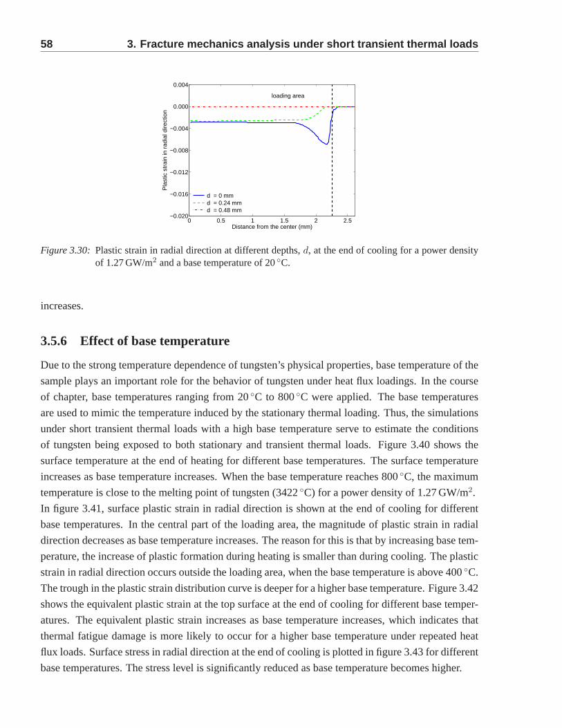
58 3. Fracture mechanics analysis under short transient the rmal loads
0 0.5 1 1.5 2 2.5−0.020
−0.016
−0.012
−0.008
−0.004
0.000
0.004
loading area
Distance from the center (mm)
Pla
stic
str
ain
in r
adia
l dire
ctio
n
d = 0 mm d = 0.24 mm d = 0.48 mm
Figure 3.30: Plastic strain in radial direction at different depths,d, at the end of cooling for a power densityof 1.27 GW/m2 and a base temperature of 20◦C.
increases.
3.5.6 Effect of base temperature
Due to the strong temperature dependence of tungsten’s physical properties, base temperature of the
sample plays an important role for the behavior of tungsten under heat flux loadings. In the course
of chapter, base temperatures ranging from 20◦C to 800◦C were applied. The base temperatures
are used to mimic the temperature induced by the stationary thermal loading. Thus, the simulations
under short transient thermal loads with a high base temperature serve to estimate the conditions
of tungsten being exposed to both stationary and transient thermal loads. Figure 3.40 shows the
surface temperature at the end of heating for different basetemperatures. The surface temperature
increases as base temperature increases. When the base temperature reaches 800◦C, the maximum
temperature is close to the melting point of tungsten (3422◦C) for a power density of 1.27 GW/m2.
In figure 3.41, surface plastic strain in radial direction isshown at the end of cooling for different
base temperatures. In the central part of the loading area, the magnitude of plastic strain in radial
direction decreases as base temperature increases. The reason for this is that by increasing base tem-
perature, the increase of plastic formation during heatingis smaller than during cooling. The plastic
strain in radial direction occurs outside the loading area,when the base temperature is above 400◦C.
The trough in the plastic strain distribution curve is deeper for a higher base temperature. Figure 3.42
shows the equivalent plastic strain at the top surface at theend of cooling for different base temper-
atures. The equivalent plastic strain increases as base temperature increases, which indicates that
thermal fatigue damage is more likely to occur for a higher base temperature under repeated heat
flux loads. Surface stress in radial direction at the end of cooling is plotted in figure 3.43 for different
base temperatures. The stress level is significantly reduced as base temperature becomes higher.
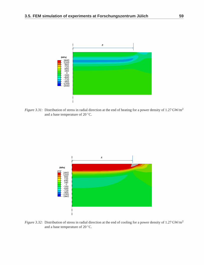
3.5. FEM simulation of experiments at Forschungszentrum Ju lich 59
Figure 3.31: Distribution of stress in radial direction at the end of heating for a power density of 1.27 GW/m2
and a base temperature of 20◦C.
Figure 3.32: Distribution of stress in radial direction at the end of cooling for a power density of 1.27 GW/m2
and a base temperature of 20◦C.
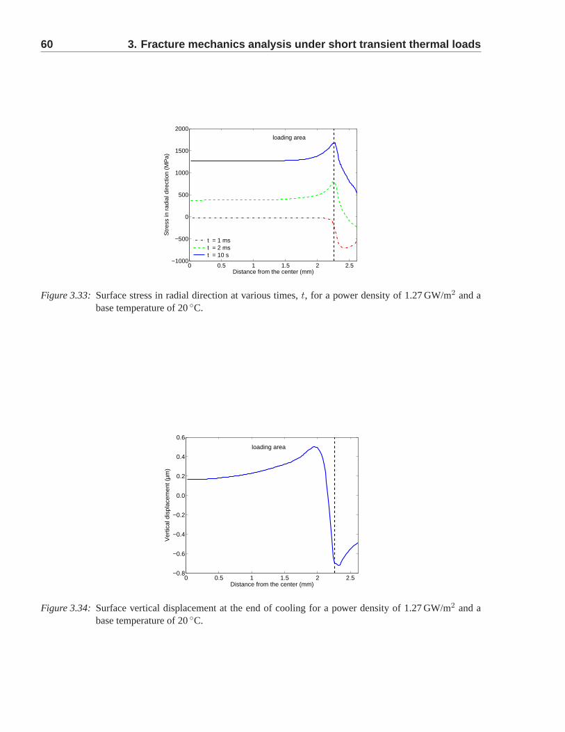
60 3. Fracture mechanics analysis under short transient the rmal loads
0 0.5 1 1.5 2 2.5−1000
−500
0
500
1000
1500
2000
loading area
Distance from the center (mm)
Str
ess
in r
adia
l dire
ctio
n (M
Pa)
t = 1 ms t = 2 ms t = 10 s
Figure 3.33: Surface stress in radial direction at various times,t, for a power density of 1.27 GW/m2 and abase temperature of 20◦C.
0 0.5 1 1.5 2 2.5−0.8
−0.6
−0.4
−0.2
0.0
0.2
0.4
0.6
loading area
Distance from the center (mm)
Ver
tical
dis
plac
emen
t (µm
)
Figure 3.34: Surface vertical displacement at the end of cooling for a power density of 1.27 GW/m2 and abase temperature of 20◦C.
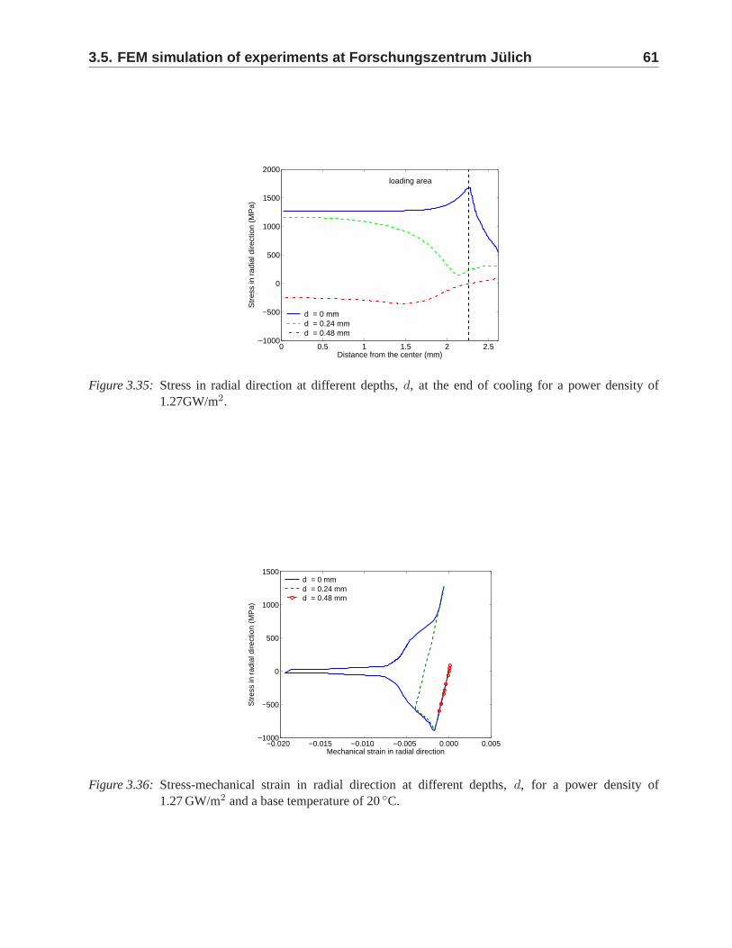
3.5. FEM simulation of experiments at Forschungszentrum Ju lich 61
0 0.5 1 1.5 2 2.5−1000
−500
0
500
1000
1500
2000
loading area
Distance from the center (mm)
Str
ess
in r
adia
l dire
ctio
n (M
Pa)
d = 0 mm d = 0.24 mm d = 0.48 mm
Figure 3.35: Stress in radial direction at different depths,d, at the end of cooling for a power density of1.27GW/m2.
−0.020 −0.015 −0.010 −0.005 0.000 0.005−1000
−500
0
500
1000
1500
Mechanical strain in radial direction
Str
ess
in r
adia
l dire
ctio
n (M
Pa)
d = 0 mm d = 0.24 mm d = 0.48 mm
Figure 3.36: Stress-mechanical strain in radial direction at different depths,d, for a power density of1.27 GW/m2 and a base temperature of 20◦C.
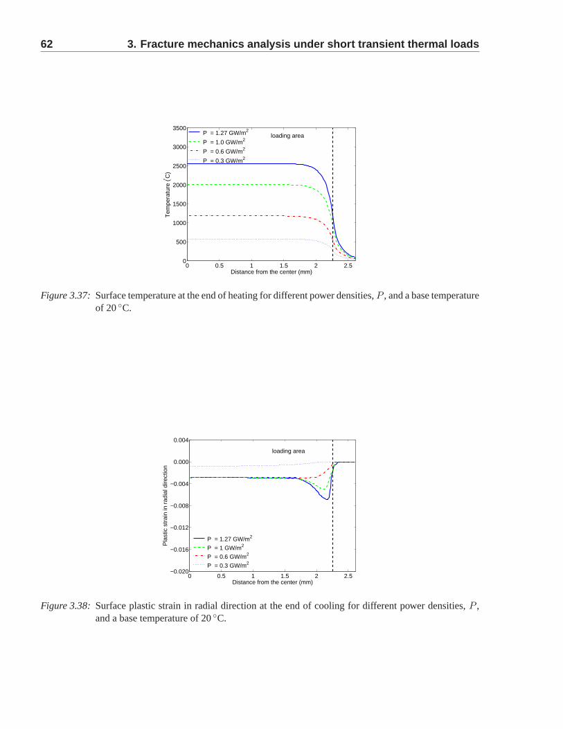
62 3. Fracture mechanics analysis under short transient the rmal loads
0 0.5 1 1.5 2 2.50
500
1000
1500
2000
2500
3000
3500loading area
Distance from the center (mm)
Tem
pera
ture
(° C)
P = 1.27 GW/m2
P = 1.0 GW/m2
P = 0.6 GW/m2
P = 0.3 GW/m2
Figure 3.37: Surface temperature at the end of heating for different power densities, P , and a base temperatureof 20◦C.
0 0.5 1 1.5 2 2.5−0.020
−0.016
−0.012
−0.008
−0.004
0.000
0.004
loading area
Distance from the center (mm)
Pla
stic
str
ain
in r
adia
l dire
ctio
n
P = 1.27 GW/m2
P = 1 GW/m2
P = 0.6 GW/m2
P = 0.3 GW/m2
Figure 3.38: Surface plastic strain in radial direction at the end of cooling for different power densities,P ,and a base temperature of 20◦C.
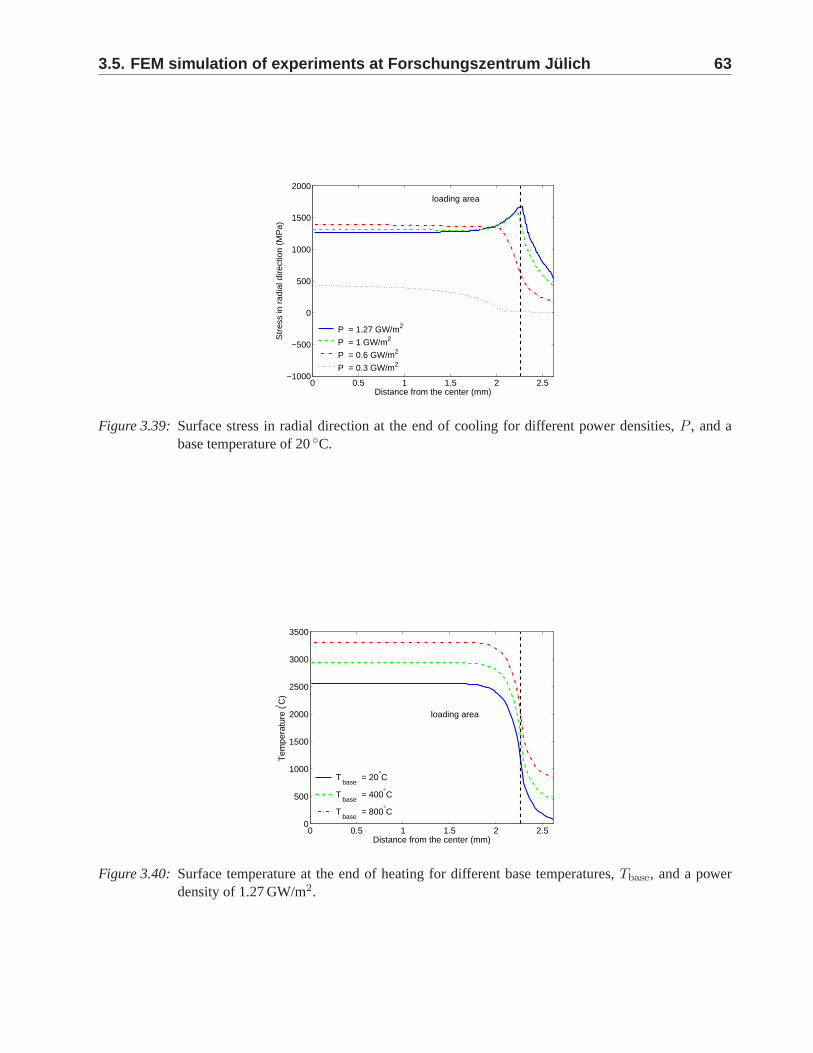
3.5. FEM simulation of experiments at Forschungszentrum Ju lich 63
0 0.5 1 1.5 2 2.5−1000
−500
0
500
1000
1500
2000
loading area
Distance from the center (mm)
Str
ess
in r
adia
l dire
ctio
n (M
Pa)
P = 1.27 GW/m2
P = 1 GW/m2
P = 0.6 GW/m2
P = 0.3 GW/m2
Figure 3.39: Surface stress in radial direction at the end of cooling for different power densities,P , and abase temperature of 20◦C.
0 0.5 1 1.5 2 2.50
500
1000
1500
2000
2500
3000
3500
loading area
Distance from the center (mm)
Tem
pera
ture
(° C)
T base
= 20°C
T base
= 400°C
T base
= 800°C
Figure 3.40: Surface temperature at the end of heating for different base temperatures,Tbase, and a powerdensity of 1.27 GW/m2.
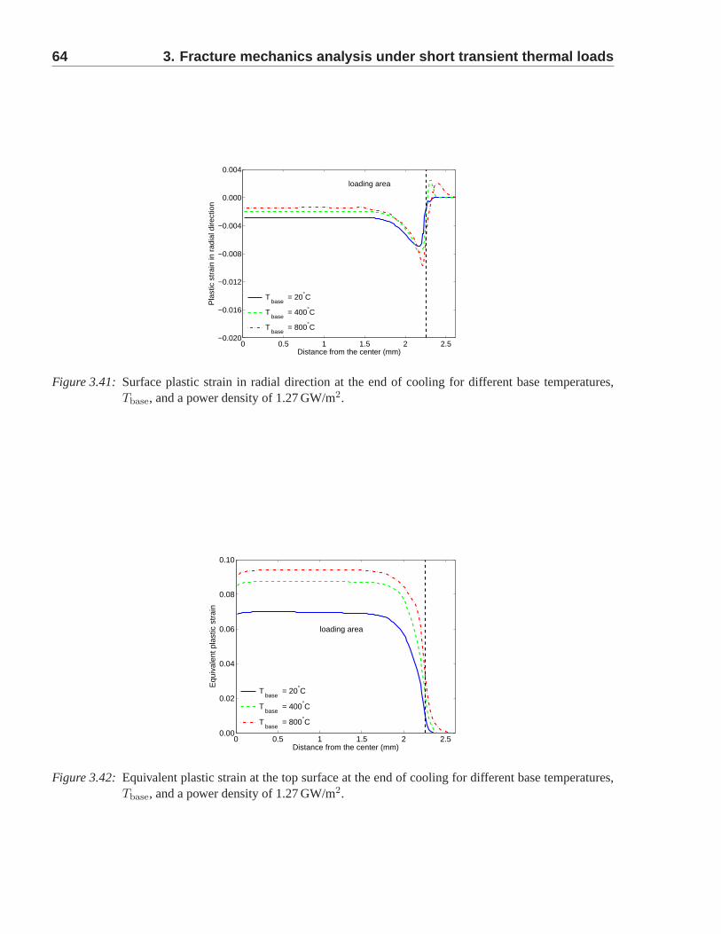
64 3. Fracture mechanics analysis under short transient the rmal loads
0 0.5 1 1.5 2 2.5−0.020
−0.016
−0.012
−0.008
−0.004
0.000
0.004
loading area
Distance from the center (mm)
Pla
stic
str
ain
in r
adia
l dire
ctio
n
T base
= 20°C
T base
= 400°C
T base
= 800°C
Figure 3.41: Surface plastic strain in radial direction at the end of cooling for different base temperatures,Tbase, and a power density of 1.27 GW/m2.
0 0.5 1 1.5 2 2.50.00
0.02
0.04
0.06
0.08
0.10
loading area
Distance from the center (mm)
Equ
ival
ent p
last
ic s
trai
n
T base
= 20°C
T base
= 400°C
T base
= 800°C
Figure 3.42: Equivalent plastic strain at the top surface at the end of cooling for different base temperatures,Tbase, and a power density of 1.27 GW/m2.
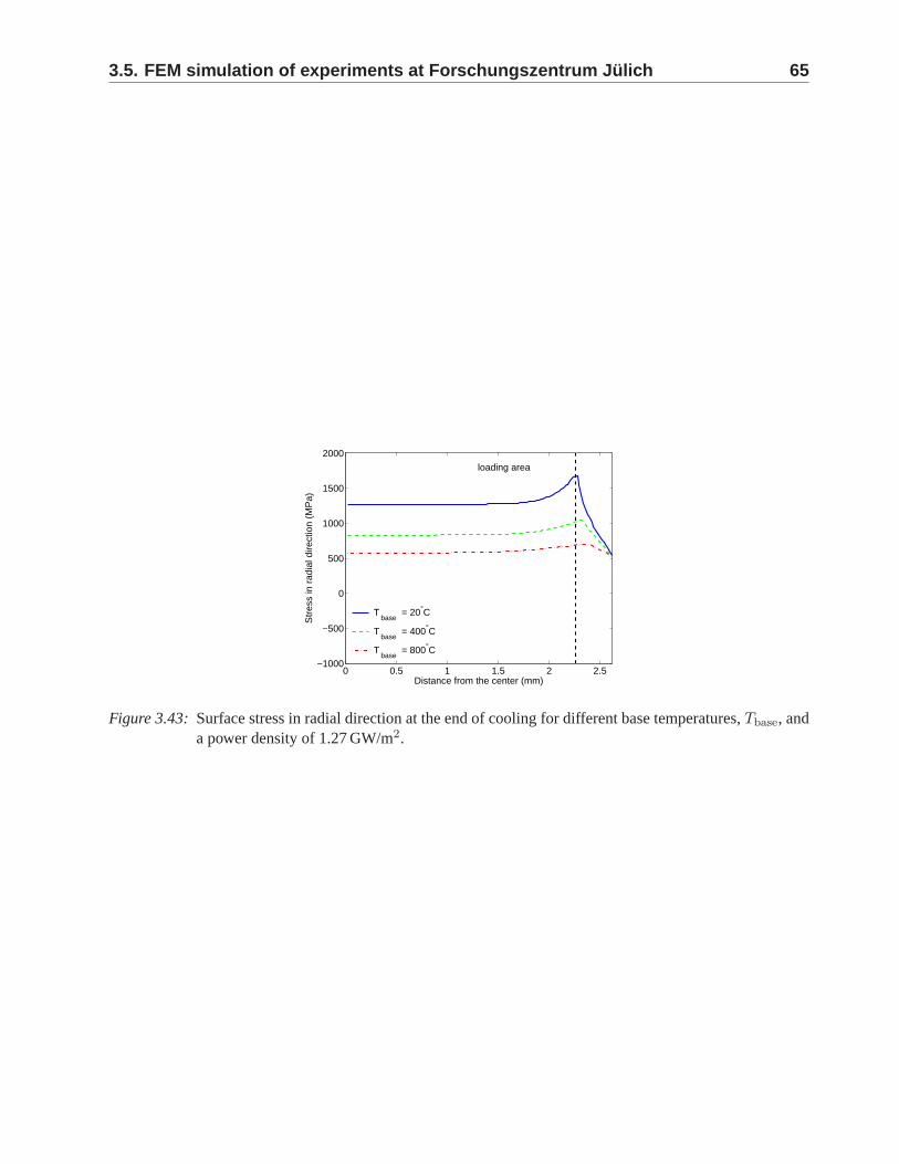
3.5. FEM simulation of experiments at Forschungszentrum Ju lich 65
0 0.5 1 1.5 2 2.5−1000
−500
0
500
1000
1500
2000
loading area
Distance from the center (mm)
Str
ess
in r
adia
l dire
ctio
n (M
Pa)
T base
= 20°C
T base
= 400°C
T base
= 800°C
Figure 3.43: Surface stress in radial direction at the end of cooling for different base temperatures,Tbase, anda power density of 1.27 GW/m2.
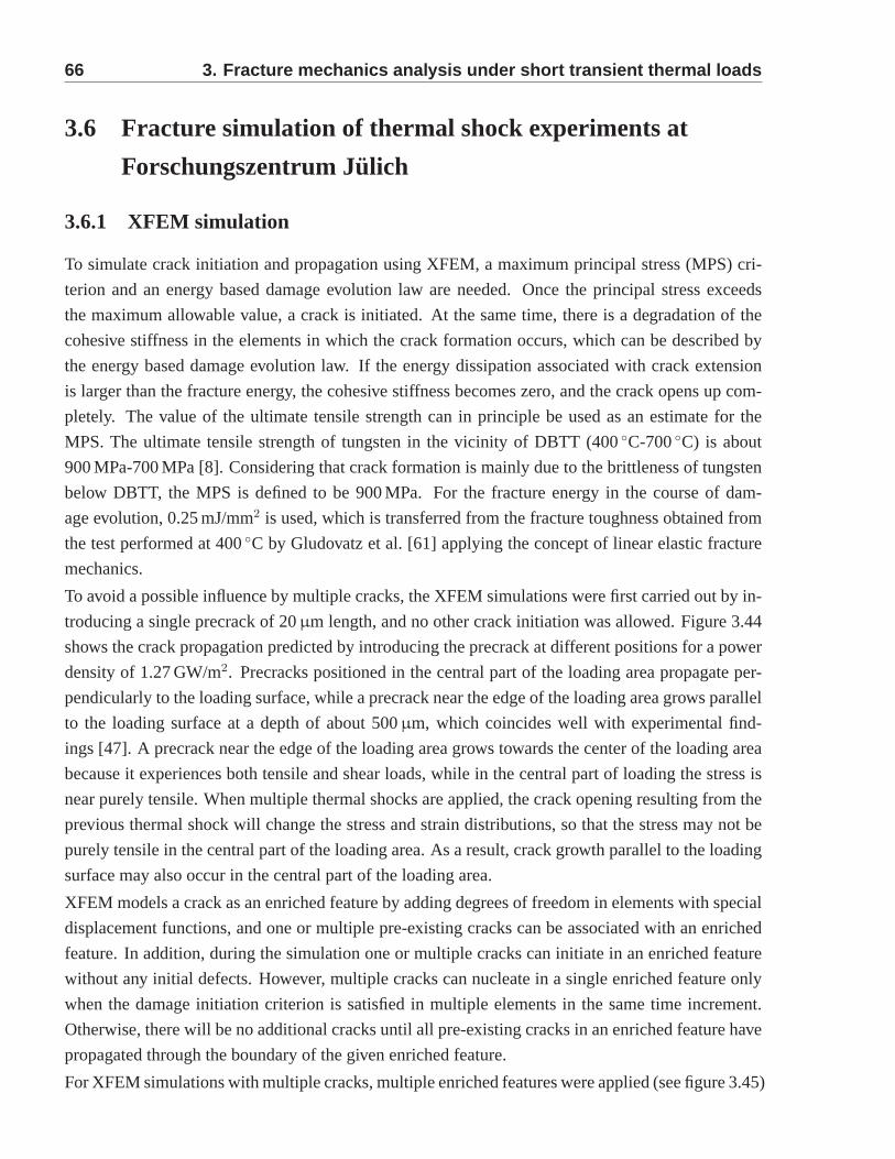
66 3. Fracture mechanics analysis under short transient the rmal loads
3.6 Fracture simulation of thermal shock experiments at
Forschungszentrum Julich
3.6.1 XFEM simulation
To simulate crack initiation and propagation using XFEM, a maximum principal stress (MPS) cri-
terion and an energy based damage evolution law are needed. Once the principal stress exceeds
the maximum allowable value, a crack is initiated. At the same time, there is a degradation of the
cohesive stiffness in the elements in which the crack formation occurs, which can be described by
the energy based damage evolution law. If the energy dissipation associated with crack extension
is larger than the fracture energy, the cohesive stiffness becomes zero, and the crack opens up com-
pletely. The value of the ultimate tensile strength can in principle be used as an estimate for the
MPS. The ultimate tensile strength of tungsten in the vicinity of DBTT (400◦C-700◦C) is about
900 MPa-700 MPa [8]. Considering that crack formation is mainly due to the brittleness of tungsten
below DBTT, the MPS is defined to be 900 MPa. For the fracture energy in the course of dam-
age evolution, 0.25 mJ/mm2 is used, which is transferred from the fracture toughness obtained from
the test performed at 400◦C by Gludovatz et al. [61] applying the concept of linear elastic fracture
mechanics.
To avoid a possible influence by multiple cracks, the XFEM simulations were first carried out by in-
troducing a single precrack of 20µm length, and no other crack initiation was allowed. Figure 3.44
shows the crack propagation predicted by introducing the precrack at different positions for a power
density of 1.27 GW/m2. Precracks positioned in the central part of the loading area propagate per-
pendicularly to the loading surface, while a precrack near the edge of the loading area grows parallel
to the loading surface at a depth of about 500µm, which coincides well with experimental find-
ings [47]. A precrack near the edge of the loading area grows towards the center of the loading area
because it experiences both tensile and shear loads, while in the central part of loading the stress is
near purely tensile. When multiple thermal shocks are applied, the crack opening resulting from the
previous thermal shock will change the stress and strain distributions, so that the stress may not be
purely tensile in the central part of the loading area. As a result, crack growth parallel to the loading
surface may also occur in the central part of the loading area.
XFEM models a crack as an enriched feature by adding degrees of freedom in elements with special
displacement functions, and one or multiple pre-existing cracks can be associated with an enriched
feature. In addition, during the simulation one or multiplecracks can initiate in an enriched feature
without any initial defects. However, multiple cracks can nucleate in a single enriched feature only
when the damage initiation criterion is satisfied in multiple elements in the same time increment.
Otherwise, there will be no additional cracks until all pre-existing cracks in an enriched feature have
propagated through the boundary of the given enriched feature.
For XFEM simulations with multiple cracks, multiple enriched features were applied (see figure 3.45)
3.6. Fracture simulation of experiments at Forschungszent rum Julich 67
Figure 3.44: Cracks predicted using XFEM with a global enriched feature and precracks at different locations(top: 0.8 mm away from the center, middle: 1.2 mm away from the center, bottom: 2.24 mmaway from the center) for a power density of 1.27 GW/m2 and a base temperature of 20◦C.The quantity STATUSXFEM characterizes damage evolution. A value of 1.0 characterizes anopened crack. Positive values smaller than 1.0 stand for cracks that require additional energy tobe opened.
so that cracks can nucleate without waiting for the pre-existing cracks to propagate in other enriched
features. Figure 3.46 shows the cracks predicted using XFEMfor loadings of different power densi-
ties. Cracks are initiated near the top surface perpendicularly to the loading surface and are not fully
opened. However, in the XFEM simulations with a single crack, the crack in central part of the load-
ing area is much longer and fully opened (see figure 3.44), since when multiple cracks are initiated
in the central part of the loading area, the stiffness is degraded in such a way that the stress concen-
tration at the crack tips is not as intensive as in the XFEM simulations with a single crack. For the
loadings with 1.27 GW/m2 and 1 GW/m2, cracks are generated near the edge of the loading area and
propagate parallel to the loading surface. For a power density of 0.6 GW/m2, no crack is formed near
the edge of the loading area, as there is no stress concentration, see figure 3.39. No crack initiation
is found for the loading with 0.3 GW/m2, since the stress is much smaller than the MPS. The XFEM
results are capable of reproducing the main cracking features observed in the experiments [47].
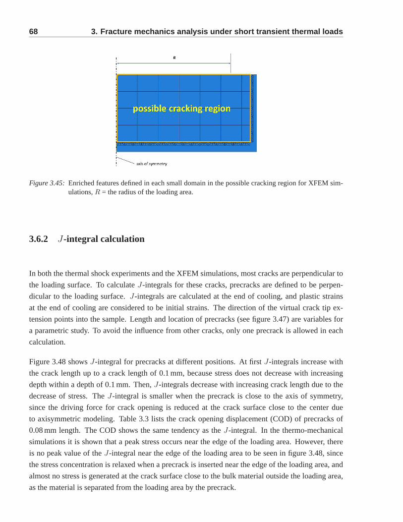
68 3. Fracture mechanics analysis under short transient the rmal loads
Figure 3.45: Enriched features defined in each small domain in the possible cracking region for XFEM sim-ulations,R = the radius of the loading area.
3.6.2 J-integral calculation
In both the thermal shock experiments and the XFEM simulations, most cracks are perpendicular to
the loading surface. To calculateJ-integrals for these cracks, precracks are defined to be perpen-
dicular to the loading surface.J-integrals are calculated at the end of cooling, and plasticstrains
at the end of cooling are considered to be initial strains. The direction of the virtual crack tip ex-
tension points into the sample. Length and location of precracks (see figure 3.47) are variables for
a parametric study. To avoid the influence from other cracks,only one precrack is allowed in each
calculation.
Figure 3.48 showsJ-integral for precracks at different positions. At firstJ-integrals increase with
the crack length up to a crack length of 0.1 mm, because stressdoes not decrease with increasing
depth within a depth of 0.1 mm. Then,J-integrals decrease with increasing crack length due to the
decrease of stress. TheJ-integral is smaller when the precrack is close to the axis ofsymmetry,
since the driving force for crack opening is reduced at the crack surface close to the center due
to axisymmetric modeling. Table 3.3 lists the crack openingdisplacement (COD) of precracks of
0.08 mm length. The COD shows the same tendency as theJ-integral. In the thermo-mechanical
simulations it is shown that a peak stress occurs near the edge of the loading area. However, there
is no peak value of theJ-integral near the edge of the loading area to be seen in figure3.48, since
the stress concentration is relaxed when a precrack is inserted near the edge of the loading area, and
almost no stress is generated at the crack surface close to the bulk material outside the loading area,
as the material is separated from the loading area by the precrack.
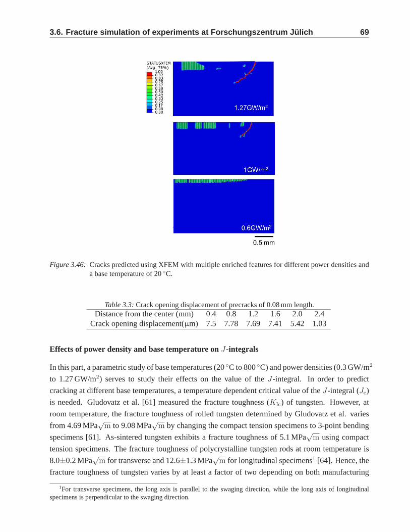
3.6. Fracture simulation of experiments at Forschungszent rum Julich 69
Figure 3.46: Cracks predicted using XFEM with multiple enriched features for differentpower densities anda base temperature of 20◦C.
Table 3.3: Crack opening displacement of precracks of 0.08 mm length.Distance from the center (mm) 0.4 0.8 1.2 1.6 2.0 2.4
Crack opening displacement(µm) 7.5 7.78 7.69 7.41 5.42 1.03
Effects of power density and base temperature onJ-integrals
In this part, a parametric study of base temperatures (20◦C to 800◦C) and power densities (0.3 GW/m2
to 1.27 GW/m2) serves to study their effects on the value of theJ-integral. In order to predict
cracking at different base temperatures, a temperature dependent critical value of theJ-integral (Jc)
is needed. Gludovatz et al. [61] measured the fracture toughness (KIc) of tungsten. However, at
room temperature, the fracture toughness of rolled tungsten determined by Gludovatz et al. varies
from 4.69 MPa√
m to 9.08 MPa√
m by changing the compact tension specimens to 3-point bending
specimens [61]. As-sintered tungsten exhibits a fracture toughness of 5.1 MPa√
m using compact
tension specimens. The fracture toughness of polycrystalline tungsten rods at room temperature is
8.0±0.2 MPa√
m for transverse and 12.6±1.3 MPa√
m for longitudinal specimens1 [64]. Hence, the
fracture toughness of tungsten varies by at least a factor oftwo depending on both manufacturing
1For transverse specimens, the long axis is parallel to the swaging direction, while the long axis of longitudinalspecimens is perpendicular to the swaging direction.
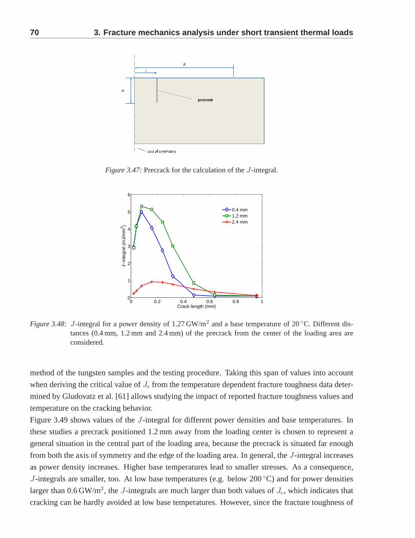
70 3. Fracture mechanics analysis under short transient the rmal loads
Figure 3.47: Precrack for the calculation of theJ-integral.
0 0.2 0.4 0.6 0.8 10
1
2
3
4
5
6
Crack length (mm)
J−in
tegr
al (
mJ/
mm
2 )
0.4 mm1.2 mm2.4 mm
Figure 3.48: J-integral for a power density of 1.27 GW/m2 and a base temperature of 20◦C. Different dis-tances (0.4 mm, 1.2 mm and 2.4 mm) of the precrack from the center of the loading area areconsidered.
method of the tungsten samples and the testing procedure. Taking this span of values into account
when deriving the critical value ofJc from the temperature dependent fracture toughness data deter-
mined by Gludovatz et al. [61] allows studying the impact of reported fracture toughness values and
temperature on the cracking behavior.
Figure 3.49 shows values of theJ-integral for different power densities and base temperatures. In
these studies a precrack positioned 1.2 mm away from the loading center is chosen to represent a
general situation in the central part of the loading area, because the precrack is situated far enough
from both the axis of symmetry and the edge of the loading area. In general, theJ-integral increases
as power density increases. Higher base temperatures lead to smaller stresses. As a consequence,
J-integrals are smaller, too. At low base temperatures (e.g.below 200◦C) and for power densities
larger than 0.6 GW/m2, theJ-integrals are much larger than both values ofJc, which indicates that
cracking can be hardly avoided at low base temperatures. However, since the fracture toughness of
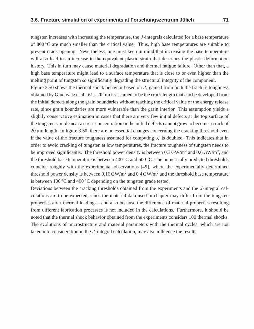
3.6. Fracture simulation of experiments at Forschungszent rum Julich 71
tungsten increases with increasing the temperature, theJ-integrals calculated for a base temperature
of 800◦C are much smaller than the critical value. Thus, high base temperatures are suitable to
prevent crack opening. Nevertheless, one must keep in mind that increasing the base temperature
will also lead to an increase in the equivalent plastic strain that describes the plastic deformation
history. This in turn may cause material degradation and thermal fatigue failure. Other than that, a
high base temperature might lead to a surface temperature that is close to or even higher than the
melting point of tungsten so significantly degrading the structural integrity of the component.
Figure 3.50 shows the thermal shock behavior based onJc gained from both the fracture toughness
obtained by Gludovatz et al. [61]. 20µm is assumed to be the crack length that can be developed from
the initial defects along the grain boundaries without reaching the critical value of the energy release
rate, since grain boundaries are more vulnerable than the grain interior. This assumption yields a
slightly conservative estimation in cases that there are very few initial defects at the top surface of
the tungsten sample near a stress concentration or the initial defects cannot grow to become a crack of
20µm length. In figure 3.50, there are no essential changes concerning the cracking threshold even
if the value of the fracture toughness assumed for computingJc is doubled. This indicates that in
order to avoid cracking of tungsten at low temperatures, thefracture toughness of tungsten needs to
be improved significantly. The threshold power density is between 0.3 GW/m2 and 0.6 GW/m2, and
the threshold base temperature is between 400◦C and 600◦C. The numerically predicted thresholds
coincide roughly with the experimental observations [49],where the experimentally determined
threshold power density is between 0.16 GW/m2 and 0.4 GW/m2 and the threshold base temperature
is between 100◦C and 400◦C depending on the tungsten grade tested.
Deviations between the cracking thresholds obtained from the experiments and theJ-integral cal-
culations are to be expected, since the material data used inchapter may differ from the tungsten
properties after thermal loadings - and also because the difference of material properties resulting
from different fabrication processes is not included in thecalculations. Furthermore, it should be
noted that the thermal shock behavior obtained from the experiments considers 100 thermal shocks.
The evolutions of microstructure and material parameters with the thermal cycles, which are not
taken into consideration in theJ-integral calculation, may also influence the results.
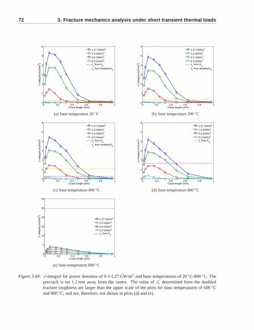
72 3. Fracture mechanics analysis under short transient the rmal loads
0 0.2 0.4 0.6 0.8 10
1
2
3
4
5
6
Crack length (mm)
J−in
tegr
al (
mJ/
mm
2 )
1.27 GW/m2
1.0 GW/m2
0.6 GW/m2
0.3 GW/m2
Jc from K
Ic
Jc from doubled K
Ic
(a) base temperature 20◦C
0 0.2 0.4 0.6 0.8 10
1
2
3
4
5
6
Crack length (mm)
J−in
tegr
al (
mJ/
mm
2 )
1.27 GW/m2
1.0 GW/m2
0.6 GW/m2
0.3 GW/m2
Jc from K
Ic
Jc from doubled K
Ic
(b) base temperature 200◦C
0 0.2 0.4 0.6 0.8 10
1
2
3
4
5
6
Crack length (mm)
J−in
tegr
al (
mJ/
mm
2 )
1.27 GW/m2
1.0 GW/m2
0.6 GW/m2
0.3 GW/m2
Jc from K
Ic
Jc from doubled K
Ic
(c) base temperature 400◦C
0 0.2 0.4 0.6 0.8 10
1
2
3
4
5
6
Crack length (mm)
J−in
tegr
al (
mJ/
mm
2 )
1.27 GW/m2
1.0 GW/m2
0.6 GW/m2
0.3 GW/m2
Jc from K
Ic
(d) base temperature 600◦C
0 0.2 0.4 0.6 0.8 10
5
10
15
20
25
30
Crack length (mm)
J−in
tegr
al (
mJ/
mm
2 )
1.27 GW/m2
1.0 GW/m2
0.6 GW/m2
0.3 GW/m2
Jc from K
Ic
(e) base temperature 800◦C
Figure 3.49: J-integral for power densities of 0.3-1.27 GW/m2 and base temperatures of 20◦C-800◦C. Theprecrack is set 1.2 mm away from the center. The value ofJc determined from the doubledfracture toughness are larger than the upper scale of the plots for basetemperatures of 600◦Cand 800◦C, and are, therefore, not shown in plots (d) and (e).
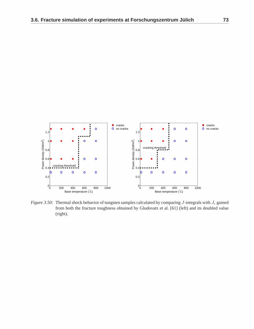
3.6. Fracture simulation of experiments at Forschungszent rum Julich 73
0 200 400 600 800 10000
0.2
0.4
0.6
0.8
1
1.2
cracking threshold
Base temperature (°C)
Pow
er d
ensi
ty (
GW
/m2 )
cracksno cracks
0 200 400 600 800 10000
0.2
0.4
0.6
0.8
1
1.2
cracking threshold
Base temperature (°C)
Pow
er d
ensi
ty (
GW
/m2 )
cracksno cracks
Figure 3.50: Thermal shock behavior of tungsten samples calculated by comparingJ-integrals withJc gainedfrom both the fracture toughness obtained by Gludovatz et al. [61] (left)and its doubled value(right).
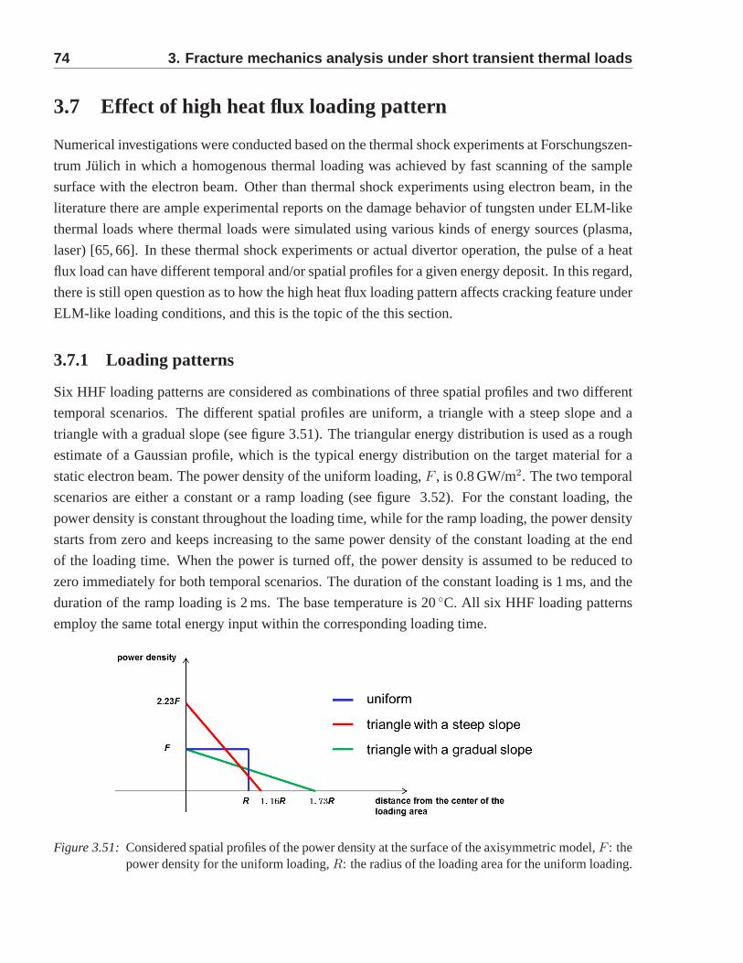
74 3. Fracture mechanics analysis under short transient the rmal loads
3.7 Effect of high heat flux loading pattern
Numerical investigations were conducted based on the thermal shock experiments at Forschungszen-
trum Julich in which a homogenous thermal loading was achieved by fast scanning of the sample
surface with the electron beam. Other than thermal shock experiments using electron beam, in the
literature there are ample experimental reports on the damage behavior of tungsten under ELM-like
thermal loads where thermal loads were simulated using various kinds of energy sources (plasma,
laser) [65, 66]. In these thermal shock experiments or actual divertor operation, the pulse of a heat
flux load can have different temporal and/or spatial profilesfor a given energy deposit. In this regard,
there is still open question as to how the high heat flux loading pattern affects cracking feature under
ELM-like loading conditions, and this is the topic of the this section.
3.7.1 Loading patterns
Six HHF loading patterns are considered as combinations of three spatial profiles and two different
temporal scenarios. The different spatial profiles are uniform, a triangle with a steep slope and a
triangle with a gradual slope (see figure 3.51). The triangular energy distribution is used as a rough
estimate of a Gaussian profile, which is the typical energy distribution on the target material for a
static electron beam. The power density of the uniform loading,F , is 0.8 GW/m2. The two temporal
scenarios are either a constant or a ramp loading (see figure 3.52). For the constant loading, the
power density is constant throughout the loading time, while for the ramp loading, the power density
starts from zero and keeps increasing to the same power density of the constant loading at the end
of the loading time. When the power is turned off, the power density is assumed to be reduced to
zero immediately for both temporal scenarios. The durationof the constant loading is 1 ms, and the
duration of the ramp loading is 2 ms. The base temperature is 20 ◦C. All six HHF loading patterns
employ the same total energy input within the correspondingloading time.
Figure 3.51: Considered spatial profiles of the power density at the surface of the axisymmetric model,F : thepower density for the uniform loading,R: the radius of the loading area for the uniform loading.
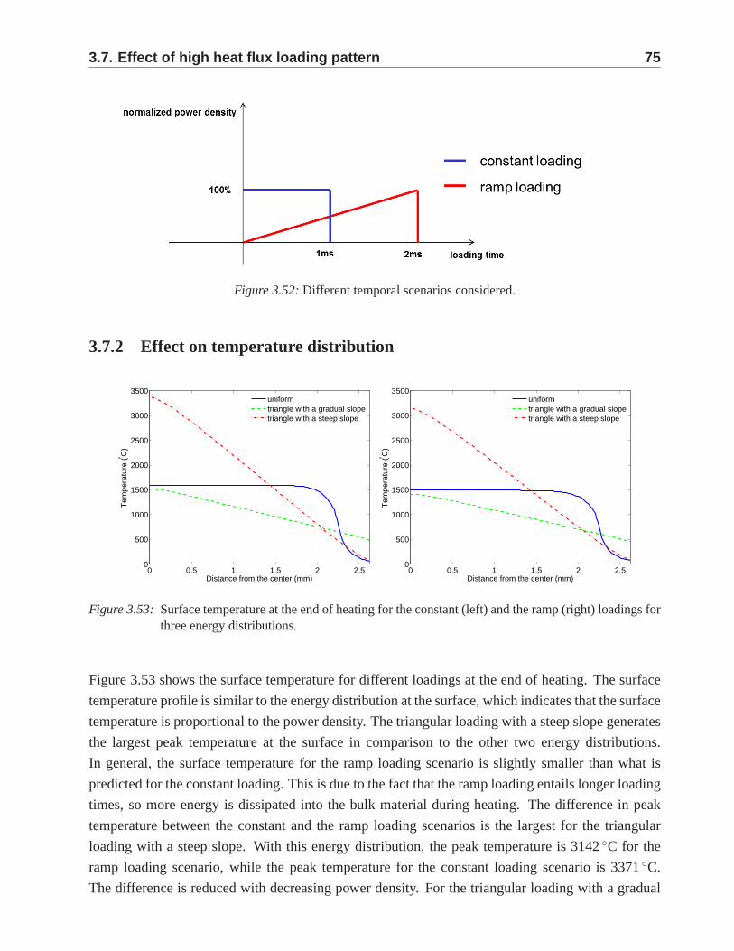
3.7. Effect of high heat flux loading pattern 75
Figure 3.52: Different temporal scenarios considered.
3.7.2 Effect on temperature distribution
0 0.5 1 1.5 2 2.50
500
1000
1500
2000
2500
3000
3500
Distance from the center (mm)
Tem
pera
ture
(° C)
uniformtriangle with a gradual slopetriangle with a steep slope
0 0.5 1 1.5 2 2.50
500
1000
1500
2000
2500
3000
3500
Distance from the center (mm)
Tem
pera
ture
(° C)
uniformtriangle with a gradual slopetriangle with a steep slope
Figure 3.53: Surface temperature at the end of heating for the constant (left) and the ramp (right) loadings forthree energy distributions.
Figure 3.53 shows the surface temperature for different loadings at the end of heating. The surface
temperature profile is similar to the energy distribution atthe surface, which indicates that the surface
temperature is proportional to the power density. The triangular loading with a steep slope generates
the largest peak temperature at the surface in comparison tothe other two energy distributions.
In general, the surface temperature for the ramp loading scenario is slightly smaller than what is
predicted for the constant loading. This is due to the fact that the ramp loading entails longer loading
times, so more energy is dissipated into the bulk material during heating. The difference in peak
temperature between the constant and the ramp loading scenarios is the largest for the triangular
loading with a steep slope. With this energy distribution, the peak temperature is 3142◦C for the
ramp loading scenario, while the peak temperature for the constant loading scenario is 3371◦C.
The difference is reduced with decreasing power density. For the triangular loading with a gradual
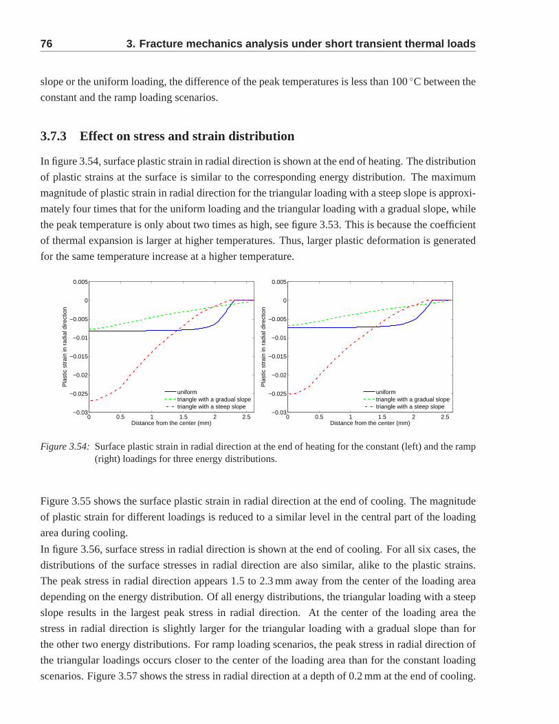
76 3. Fracture mechanics analysis under short transient the rmal loads
slope or the uniform loading, the difference of the peak temperatures is less than 100◦C between the
constant and the ramp loading scenarios.
3.7.3 Effect on stress and strain distribution
In figure 3.54, surface plastic strain in radial direction isshown at the end of heating. The distribution
of plastic strains at the surface is similar to the corresponding energy distribution. The maximum
magnitude of plastic strain in radial direction for the triangular loading with a steep slope is approxi-
mately four times that for the uniform loading and the triangular loading with a gradual slope, while
the peak temperature is only about two times as high, see figure 3.53. This is because the coefficient
of thermal expansion is larger at higher temperatures. Thus, larger plastic deformation is generated
for the same temperature increase at a higher temperature.
0 0.5 1 1.5 2 2.5−0.03
−0.025
−0.02
−0.015
−0.01
−0.005
0
0.005
Distance from the center (mm)
Pla
stic
str
ain
in r
adia
l dire
ctio
n
uniformtriangle with a gradual slopetriangle with a steep slope
0 0.5 1 1.5 2 2.5−0.03
−0.025
−0.02
−0.015
−0.01
−0.005
0
0.005
Distance from the center (mm)
Pla
stic
str
ain
in r
adia
l dire
ctio
n
uniformtriangle with a gradual slopetriangle with a steep slope
Figure 3.54: Surface plastic strain in radial direction at the end of heating for the constant (left) and the ramp(right) loadings for three energy distributions.
Figure 3.55 shows the surface plastic strain in radial direction at the end of cooling. The magnitude
of plastic strain for different loadings is reduced to a similar level in the central part of the loading
area during cooling.
In figure 3.56, surface stress in radial direction is shown atthe end of cooling. For all six cases, the
distributions of the surface stresses in radial direction are also similar, alike to the plastic strains.
The peak stress in radial direction appears 1.5 to 2.3 mm awayfrom the center of the loading area
depending on the energy distribution. Of all energy distributions, the triangular loading with a steep
slope results in the largest peak stress in radial direction. At the center of the loading area the
stress in radial direction is slightly larger for the triangular loading with a gradual slope than for
the other two energy distributions. For ramp loading scenarios, the peak stress in radial direction of
the triangular loadings occurs closer to the center of the loading area than for the constant loading
scenarios. Figure 3.57 shows the stress in radial directionat a depth of 0.2 mm at the end of cooling.
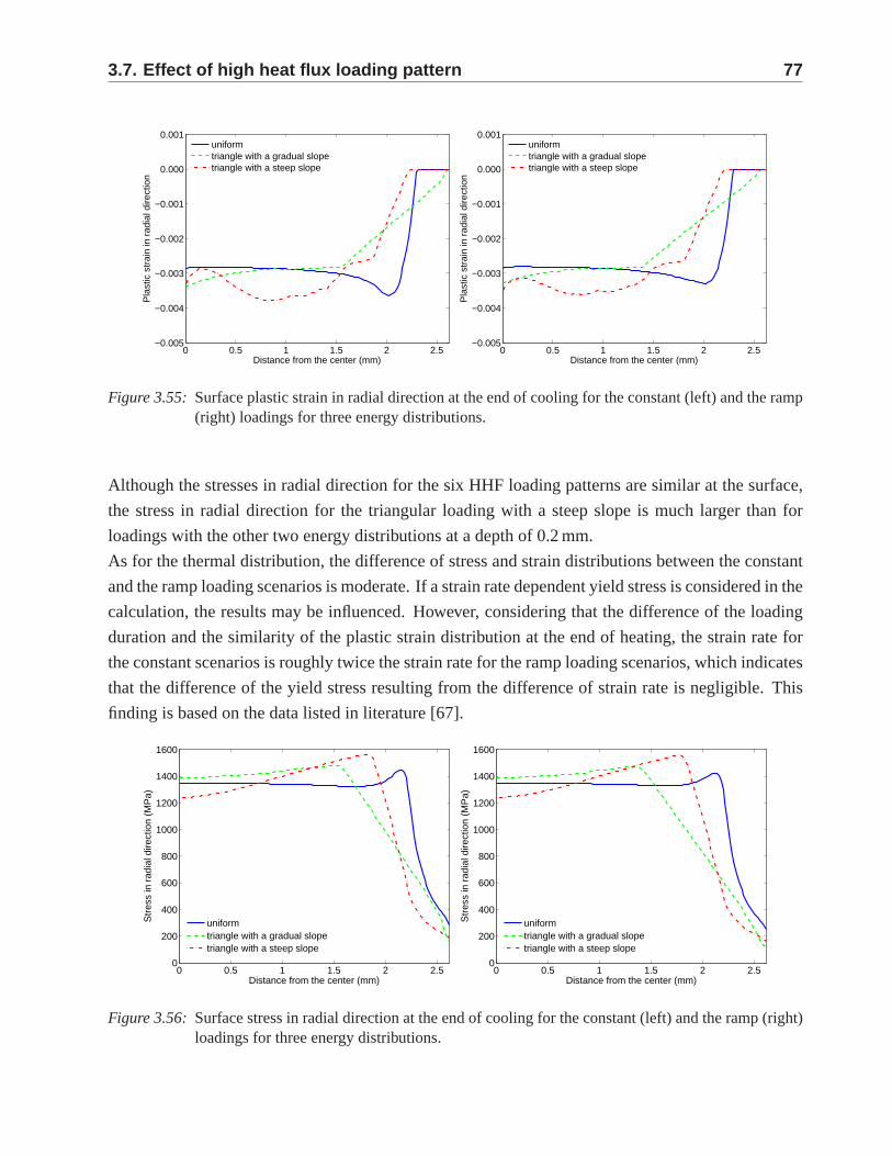
3.7. Effect of high heat flux loading pattern 77
0 0.5 1 1.5 2 2.5−0.005
−0.004
−0.003
−0.002
−0.001
0.000
0.001
Distance from the center (mm)
Pla
stic
str
ain
in r
adia
l dire
ctio
n
uniformtriangle with a gradual slopetriangle with a steep slope
0 0.5 1 1.5 2 2.5−0.005
−0.004
−0.003
−0.002
−0.001
0.000
0.001
Distance from the center (mm)
Pla
stic
str
ain
in r
adia
l dire
ctio
n
uniformtriangle with a gradual slopetriangle with a steep slope
Figure 3.55: Surface plastic strain in radial direction at the end of cooling for the constant (left) and the ramp(right) loadings for three energy distributions.
Although the stresses in radial direction for the six HHF loading patterns are similar at the surface,
the stress in radial direction for the triangular loading with a steep slope is much larger than for
loadings with the other two energy distributions at a depth of 0.2 mm.
As for the thermal distribution, the difference of stress and strain distributions between the constant
and the ramp loading scenarios is moderate. If a strain rate dependent yield stress is considered in the
calculation, the results may be influenced. However, considering that the difference of the loading
duration and the similarity of the plastic strain distribution at the end of heating, the strain rate for
the constant scenarios is roughly twice the strain rate for the ramp loading scenarios, which indicates
that the difference of the yield stress resulting from the difference of strain rate is negligible. This
finding is based on the data listed in literature [67].
0 0.5 1 1.5 2 2.50
200
400
600
800
1000
1200
1400
1600
Distance from the center (mm)
Str
ess
in r
adia
l dire
ctio
n (M
Pa)
uniformtriangle with a gradual slopetriangle with a steep slope
0 0.5 1 1.5 2 2.50
200
400
600
800
1000
1200
1400
1600
Distance from the center (mm)
Str
ess
in r
adia
l dire
ctio
n (M
Pa)
uniformtriangle with a gradual slopetriangle with a steep slope
Figure 3.56: Surface stress in radial direction at the end of cooling for the constant (left) and the ramp (right)loadings for three energy distributions.
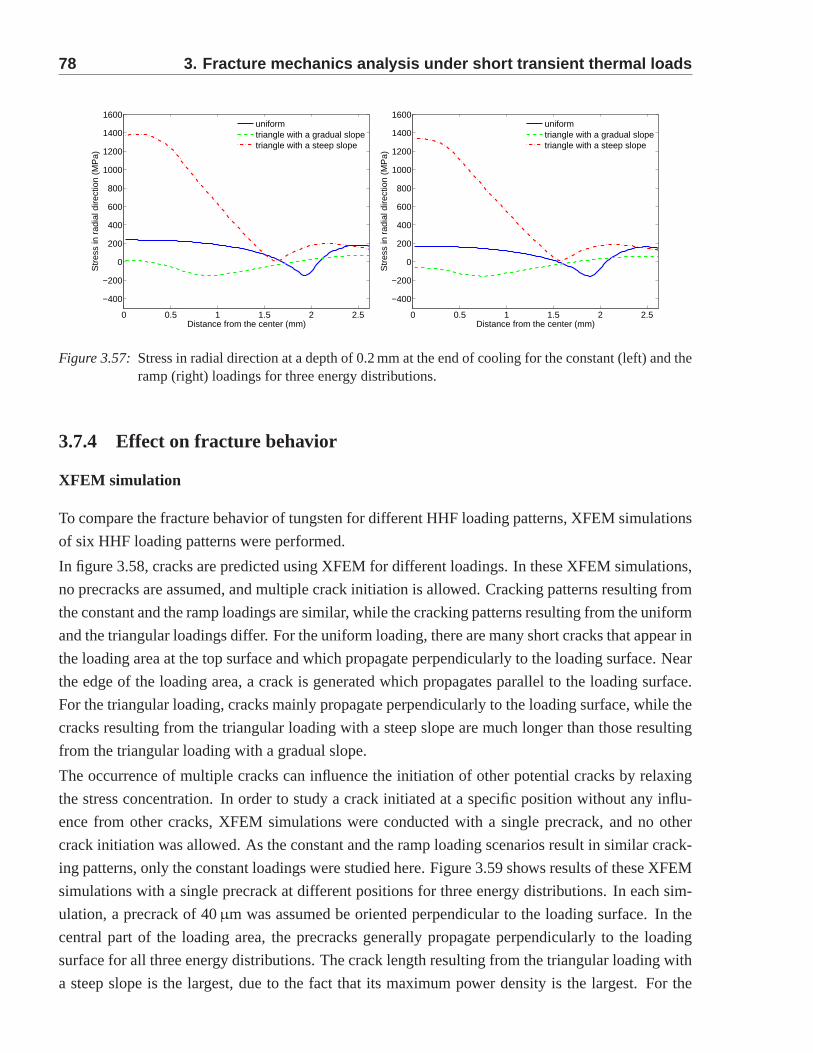
78 3. Fracture mechanics analysis under short transient the rmal loads
0 0.5 1 1.5 2 2.5
−400
−200
0
200
400
600
800
1000
1200
1400
1600
Distance from the center (mm)
Str
ess
in r
adia
l dire
ctio
n (M
Pa)
uniformtriangle with a gradual slopetriangle with a steep slope
0 0.5 1 1.5 2 2.5
−400
−200
0
200
400
600
800
1000
1200
1400
1600
Distance from the center (mm)
Str
ess
in r
adia
l dire
ctio
n (M
Pa)
uniformtriangle with a gradual slopetriangle with a steep slope
Figure 3.57: Stress in radial direction at a depth of 0.2 mm at the end of cooling for the constant (left) and theramp (right) loadings for three energy distributions.
3.7.4 Effect on fracture behavior
XFEM simulation
To compare the fracture behavior of tungsten for different HHF loading patterns, XFEM simulations
of six HHF loading patterns were performed.
In figure 3.58, cracks are predicted using XFEM for differentloadings. In these XFEM simulations,
no precracks are assumed, and multiple crack initiation is allowed. Cracking patterns resulting from
the constant and the ramp loadings are similar, while the cracking patterns resulting from the uniform
and the triangular loadings differ. For the uniform loading, there are many short cracks that appear in
the loading area at the top surface and which propagate perpendicularly to the loading surface. Near
the edge of the loading area, a crack is generated which propagates parallel to the loading surface.
For the triangular loading, cracks mainly propagate perpendicularly to the loading surface, while the
cracks resulting from the triangular loading with a steep slope are much longer than those resulting
from the triangular loading with a gradual slope.
The occurrence of multiple cracks can influence the initiation of other potential cracks by relaxing
the stress concentration. In order to study a crack initiated at a specific position without any influ-
ence from other cracks, XFEM simulations were conducted with a single precrack, and no other
crack initiation was allowed. As the constant and the ramp loading scenarios result in similar crack-
ing patterns, only the constant loadings were studied here.Figure 3.59 shows results of these XFEM
simulations with a single precrack at different positions for three energy distributions. In each sim-
ulation, a precrack of 40µm was assumed be oriented perpendicular to the loading surface. In the
central part of the loading area, the precracks generally propagate perpendicularly to the loading
surface for all three energy distributions. The crack length resulting from the triangular loading with
a steep slope is the largest, due to the fact that its maximum power density is the largest. For the
3.7. Effect of high heat flux loading pattern 79
triangular loading with a steep slope and a precrack positioned 2.01 mm from the center of the load-
ing area makes it propagate parallel to the loading surface,i.e. deviate from its initial vertical path.
A similar crack is found 2.23 mm away from the center of the loading area for the uniform loading.
For the triangular loading with a gradual slope, the precrack 1.61 mm away from the center of the
loading area tends to propagate towards the center of the loading area, but the driving force is not
large enough for significant crack growth.
As shown in figure 3.59, cracks are found near the position where the peak stress occurs for the
uniform and triangular loadings with a steep slope (XFEM simulations with a single precrack).
These cracks propagate parallel to the loading surface. However, cracks do not propagate parallel
to the loading surface for the triangular loading with a steep slope, if multiple crack initiations are
allowed, see figure 3.58. This is due to the stress relaxationresulting from the crack opening in the
central part of the loading area. To confirm this conclusion,the XFEM simulations were made with
two precracks at specific positions. One precrack was definedin the central part of the loading area
(d = 0.81 mm) while the other precrack was defined near the position where the peak stress occurs.
The results of these calculations are shown in figure 3.60. Crack propagation parallel to the loading
surface is hindered as crack opening occurs in the central part of the loading area. This indicates that
for power densities sufficiently large to induce cracking inthe central part of the loading area, crack
growth parallel to the loading surface will be impeded. If the power density is too small, no cracking
will occur. For the aforementioned reasons the cracking pattern predicted for the uniform loading in
figure 3.58 occurs within a certain range of the power density, which allows the occurrence of the
cracks near the edge of the loading area but does not lead to serious cracking in the central part of the
loading area. This cracking pattern should be avoided, since it may lead an undesired concentration
of thermal energy at the top surface and subsequent melting or erosion of surface material.
Compared to the triangular loading, the uniform loading is more likely to cause a crack near the
position where the peak stress occurs and which will grow parallel to the loading surface. On one
hand, the distance between the position of peak stress and the loading center is larger for the uniform
loading than for the triangular loading, which indicates that the growth of cracks near the edge of
the loading area is less influenced by cracking in the centralpart, see figure 3.60. On the other hand,
the uniformly distributed stress distribution under the uniform loading can create many short cracks
in the central part of the loading area at the same time, whichreduces the driving force for a long
crack, see figure 3.58.
J-integral calculation
TheJ-integral is calculated for precracks of various lengths atdifferent positions in order to compile
a parametric study, see figure 3.61. In each calculation, a single precrack is defined with a fixed
length. The critical value of theJ-integral (Jc) is assumed to be the same as the fracture energy
used in the XFEM simulations. The direction of the virtual crack tip extension is downwards and
perpendicular to the loading surface.
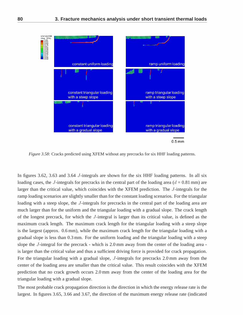
80 3. Fracture mechanics analysis under short transient the rmal loads
Figure 3.58: Cracks predicted using XFEM without any precracks for six HHF loadingpatterns.
In figures 3.62, 3.63 and 3.64J-integrals are shown for the six HHF loading patterns. In allsix
loading cases, theJ-integrals for precracks in the central part of the loading area (d = 0.81 mm) are
larger than the critical value, which coincides with the XFEM prediction. TheJ-integrals for the
ramp loading scenarios are slightly smaller than for the constant loading scenarios. For the triangular
loading with a steep slope, theJ-integrals for precracks in the central part of the loading area are
much larger than for the uniform and the triangular loading with a gradual slope. The crack length
of the longest precrack, for which theJ-integral is larger than its critical value, is defined as the
maximum crack length. The maximum crack length for the triangular loading with a steep slope
is the largest (approx. 0.6 mm), while the maximum crack length for the triangular loading with a
gradual slope is less than 0.3 mm. For the uniform loading andthe triangular loading with a steep
slope theJ-integral for the precrack - which is 2.0 mm away from the center of the loading area -
is larger than the critical value and thus a sufficient driving force is provided for crack propagation.
For the triangular loading with a gradual slope,J-integrals for precracks 2.0 mm away from the
center of the loading area are smaller than the critical value. This result coincides with the XFEM
prediction that no crack growth occurs 2.0 mm away from the center of the loading area for the
triangular loading with a gradual slope.
The most probable crack propagation direction is the direction in which the energy release rate is the
largest. In figures 3.65, 3.66 and 3.67, the direction of the maximum energy release rate (indicated
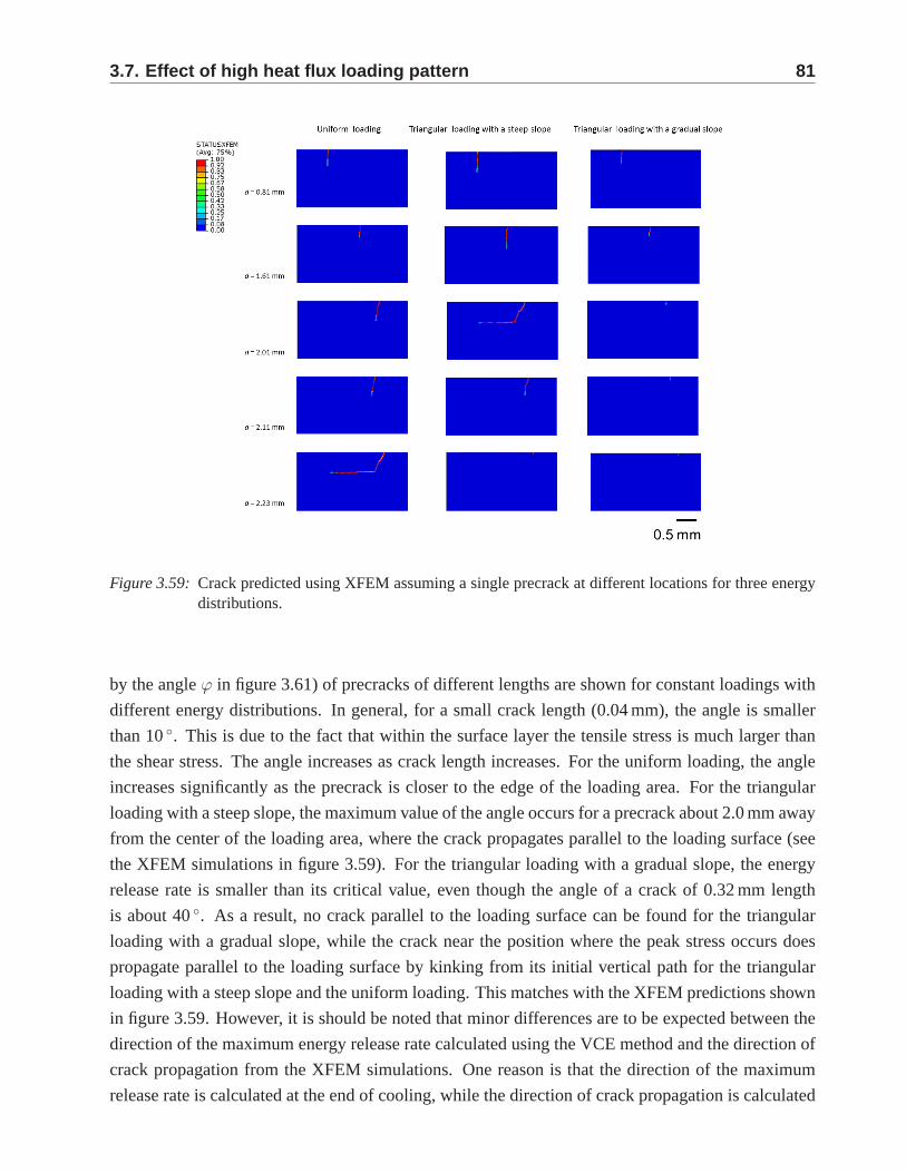
3.7. Effect of high heat flux loading pattern 81
Figure 3.59: Crack predicted using XFEM assuming a single precrack at different locations for three energydistributions.
by the angleϕ in figure 3.61) of precracks of different lengths are shown for constant loadings with
different energy distributions. In general, for a small crack length (0.04 mm), the angle is smaller
than 10◦. This is due to the fact that within the surface layer the tensile stress is much larger than
the shear stress. The angle increases as crack length increases. For the uniform loading, the angle
increases significantly as the precrack is closer to the edgeof the loading area. For the triangular
loading with a steep slope, the maximum value of the angle occurs for a precrack about 2.0 mm away
from the center of the loading area, where the crack propagates parallel to the loading surface (see
the XFEM simulations in figure 3.59). For the triangular loading with a gradual slope, the energy
release rate is smaller than its critical value, even thoughthe angle of a crack of 0.32 mm length
is about 40◦. As a result, no crack parallel to the loading surface can be found for the triangular
loading with a gradual slope, while the crack near the position where the peak stress occurs does
propagate parallel to the loading surface by kinking from its initial vertical path for the triangular
loading with a steep slope and the uniform loading. This matches with the XFEM predictions shown
in figure 3.59. However, it is should be noted that minor differences are to be expected between the
direction of the maximum energy release rate calculated using the VCE method and the direction of
crack propagation from the XFEM simulations. One reason is that the direction of the maximum
release rate is calculated at the end of cooling, while the direction of crack propagation is calculated
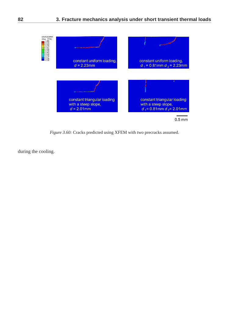
82 3. Fracture mechanics analysis under short transient the rmal loads
Figure 3.60: Cracks predicted using XFEM with two precracks assumed.
during the cooling.
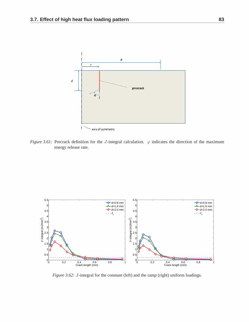
3.7. Effect of high heat flux loading pattern 83
Figure 3.61: Precrack definition for theJ-integral calculation.ϕ indicates the direction of the maximumenergy release rate.
0 0.2 0.4 0.6 0.8 10
0.5
1
1.5
2
2.5
3
3.5
4
4.5
5
5.5
Crack length (mm)
J−in
tegr
al (
mJ/
mm
2 )
d=0.8 mmd=1.6 mmd=2.0 mmJ
c
0 0.2 0.4 0.6 0.8 10
0.5
1
1.5
2
2.5
3
3.5
4
4.5
5
5.5
Crack length (mm)
J−in
tegr
al (
mJ/
mm
2 )
d=0.8 mmd=1.6 mmd=2.0 mmJ
c
Figure 3.62: J-integral for the constant (left) and the ramp (right) uniform loadings.
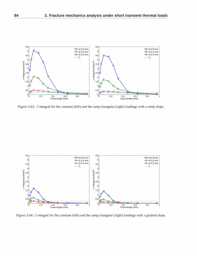
84 3. Fracture mechanics analysis under short transient the rmal loads
0 0.2 0.4 0.6 0.8 10
0.5
1
1.5
2
2.5
3
3.5
4
4.5
5
5.5
Crack length (mm)
J−in
tegr
al (
mJ/
mm
2 )
d=0.8 mmd=1.6 mmd=2.0 mmJ
c
0 0.2 0.4 0.6 0.8 10
0.5
1
1.5
2
2.5
3
3.5
4
4.5
5
5.5
Crack length (mm)
J−in
tegr
al (
mJ/
mm
2 )
d=0.8 mmd=1.6 mmd=2.0 mmJ
c
Figure 3.63: J-integral for the constant (left) and the ramp triangular (right) loadings witha steep slope.
0 0.2 0.4 0.6 0.8 10
0.5
1
1.5
2
2.5
3
3.5
4
4.5
5
5.5
Crack length (mm)
J−in
tegr
al (
mJ/
mm
2 )
d=0.8 mmd=1.6 mmd=2.0 mmJ
c
0 0.2 0.4 0.6 0.8 10
0.5
1
1.5
2
2.5
3
3.5
4
4.5
5
5.5
Crack length (mm)
J−in
tegr
al (
mJ/
mm
2 )
d=0.8 mmd=1.6 mmd=2.0 mmJ
c
Figure 3.64: J-integral for the constant (left) and the ramp triangular (right) loadings with agradual slope.
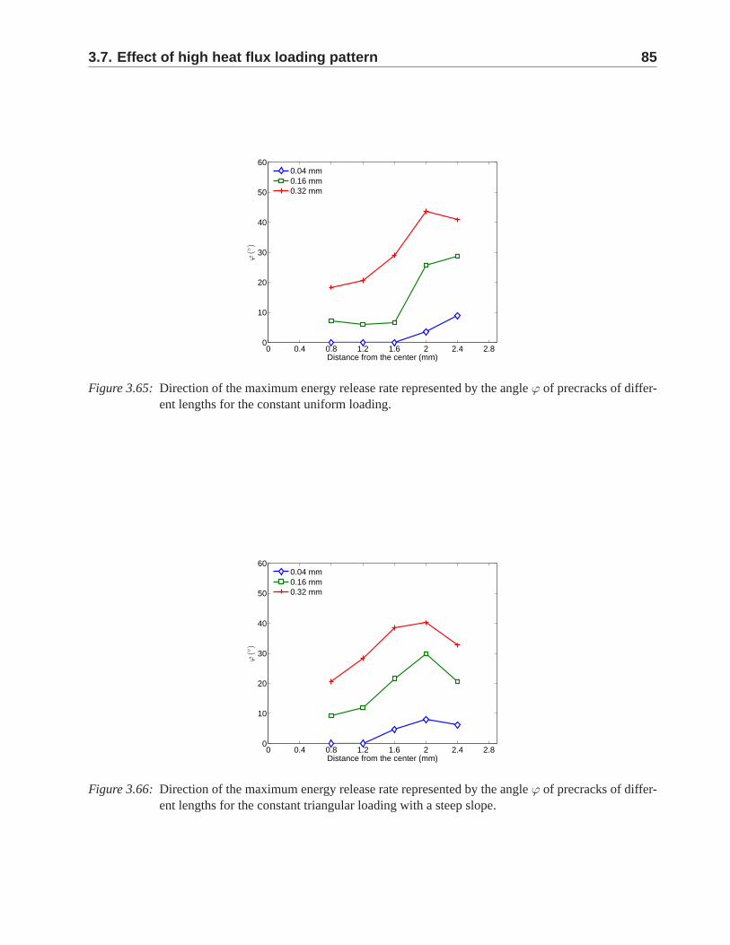
3.7. Effect of high heat flux loading pattern 85
0 0.4 0.8 1.2 1.6 2 2.4 2.80
10
20
30
40
50
60
Distance from the center (mm)
ϕ(◦
)
0.04 mm0.16 mm0.32 mm
Figure 3.65: Direction of the maximum energy release rate represented by the angleϕ of precracks of differ-ent lengths for the constant uniform loading.
0 0.4 0.8 1.2 1.6 2 2.4 2.80
10
20
30
40
50
60
Distance from the center (mm)
ϕ(◦
)
0.04 mm0.16 mm0.32 mm
Figure 3.66: Direction of the maximum energy release rate represented by the angleϕ of precracks of differ-ent lengths for the constant triangular loading with a steep slope.
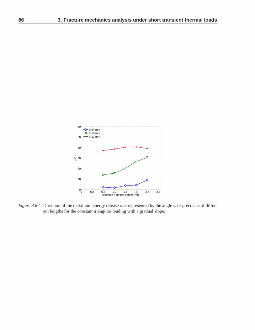
86 3. Fracture mechanics analysis under short transient the rmal loads
0 0.4 0.8 1.2 1.6 2 2.4 2.80
10
20
30
40
50
60
Distance from the center (mm)
ϕ(◦
)
0.04 mm0.16 mm0.32 mm
Figure 3.67: Direction of the maximum energy release rate represented by the angleϕ of precracks of differ-ent lengths for the constant triangular loading with a gradual slope.
3.8. Summary 87
3.8 Summary
This chapter focused on a fracture mechanics analysis of tungsten under short transient thermal loads
by ELMs, based on analytical and numerical calculations.
It was assumed that the solution assuming a semi-infinite space can give a good estimation of the
behavior of tungsten in the central part of the loading area in the ELM-like thermal shocks tests, since
the loading was nearly homogenous in the loading area. As a result, a simplified analytical solution
was derived to capture the temperature, strain and stress distributions in a semi-infinite space. This
analytical solution matched the numerical solution very well. By introducing the weight function
of a semi-infinite space solution, the stress intensity factor was calculated for the prospective crack.
Generally, the failure map based on the comparison of stressintensity factors and fracture toughness
coincided with the experimental observations.
Other than analytical estimations, a comprehensive computational study of thermo-mechanical and
fracture behaviors of tungsten under ELM-like thermal shocks was presented. A series of parametric
simulations were conducted using an axisymmetric model based on elasto-plastic finite element
analysis. The effects of power density and base temperatureon the temperature, stress and strain
distributions were evaluated. Based on the thermal simulations, a failure modeling on tungsten under
ELM-like thermal shocks was conducted. Crack initiation andpropagation were simulated using
XFEM, while theJ-integrals, which represent the energy release rate at crack tips, were evaluated
using the FEM-based VCE method. The following features of tungsten behavior were found under
ELM-like thermal shocks:
1. Upon cooling, tensile stress develops in the loaded surface layer as a consequence of plastic flow,
coined as residual stress at the end of the cooling process. The radial component of tensile stress
shows its maximum peak at the boundary of the loading area. Atthis position, a crack most
probably first propagates in vertical direction, followed by a gradual horizontal kinking, parallel
to the loading surface. Such cracking characteristics are typical for a power density of 1 GW/m2
and higher.
2. There is a threshold value of the heat flux load above which significant plastic flow takes place
during both heating and cooling - and above which almost identical plastic strain and tensile stress
are generated at the end of cooling. This threshold ranges between 0.3 GW/m2 and 0.6 GW/m2 at
a base temperature of 20◦C.
3. The maximum peak value of the tensile residual stress (radial component) increases as the power
density of the heat load is increased.
4. When the critical stress for crack initiation is reduced, many small cracks are formed in perpen-
dicular direction to the surface over the whole loading area, especially in the central region. Once
these cracks are initiated and continue to grow in the central part, the driving force for cracking
near the boundary of the loading area is reduced.
88 3. Fracture mechanics analysis under short transient the rmal loads
5. The crack formation is predicted for the power density of 0.6 GW/m2 and above, and when the
base temperature is higher than 600◦C, almost no crack is predicted.
6. The predicted threshold values of power density and base temperature for cracking agree roughly
with the experimental observations. There are no essentialchanges concerning the cracking
threshold even if the value of fracture toughness assumed for the simulation is increased by a
factor of two.
The last part of the chapter dealt with the influence of loading patterns of ELM-like transient thermal
loads on the fracture behavior of tungsten. Comparative assessment of initial cracking and crack
growth was conducted for six HHF loading patterns (combinations of three spatial and two temporal
variants) assuming the same deposited energy for all cases.Several distinct effects were found.
1. A ramp pulse with a longer duration leads to lower temperatures and stresses in comparison
to a constant pulse with a shorter duration. Yet, the difference is moderate when both their
maximum power density and total deposited energy are identical. No significant deviation of
cracking between these two temporal loading scenarios can be observed.
2. Cracks in the central part of the loading area are initiatedin perpendicular orientation to the
surface. The final length of these cracks is dependent on the applied power density. Thus, the
length of the crack produced under the triangular loading profile with a steep slope is larger than
those of the triangular profile with a gradual slope and of theuniform distribution.
3. Regardless of the thermal loading distribution, cracks produced near the position where the peak
stress occurs tend to kink from their initial vertical path at a certain depth (e.g. 0.32 mm) and
grow further in parallel to the surface.
4. Cracks initiated near the position where the peak stress occurs are more likely to grow further in
parallel to the surface under the uniform loading, comparedto the triangular loading.
89
Chapter 4
Fracture mechanics analysis of tungsten
under slow high-energy-deposition thermal
loads
4.1 Vertical displacement events
Besides the ELMs, PFCs will have to withstand slow high-energy-deposition thermal loads, which
are characterized by a significantly longer duration than the ELMs. Vertical displacement events
(VDEs) are a typical example for such events. A VDE is an uncontrolled growth of the plasma
unstable vertical mode. The plasma has a tendency to be inherently instable and consequently ef-
fecting small vertical displacements due to the non-circular cross-section of the plasma confinement.
Although, during operation of the fusion reactor, the plasma is always vertically controlled, such un-
controlled growths can occur for various reasons, for example [68]:
• fast disturbances acting on a time scale which is outside the control system bandwidth;
• delays in the control loop;
• wrong control action due to measurement noise, when plasmavelocity is almost zero.
As a result, the plasma can then move vertically up or down and- in extreme cases - even contact with
the vessel wall, which leads to a high-energy-deposition thermal loading on the PFCs. The typical
pulse duration of VDEs ranges from 100 to 300 ms [69], which isnearly three magnitudes higher
than the pulse duration of the ELMs. Such an event with deposited energy densities of 60 MJ/m2
will cause the PFC’s surface to melt and entail a loss of the PFM, which were observed in the VDE
tests on water-cooled PFCs with active cooling of the heat sink performed by Linke et al. [69].
For analytical evaluation, Cardella et al. [70] have calculated the amount of melted and evaporated
material, taking into account the evolution of the evaporated and melted layer and in order to assess
90 4. Fracture mechanics analysis under slow high-energy-d eposition loads
possible effects of local temporary loss of cooling. Due to severe surface melting, erosion and
substantial damage on the PFCs, only a few of these events can be tolerated. Thus, special measures
must be taken so that no melting of the PFMs occurs or the melted PFMs under the VDEs do not
lose their functionality. However, it is currently difficult to predict the VDEs in detail because of its
uncertainty. Nevertheless, assuming there is a way to limitthe thermal loading induced by the VDEs
to an area that is sufficiently small, the temperature will not exceed the melting point of tungsten.
In this sense, it is also of interest to assess the material behavior in this limited loading area. In this
chapter, the thermo-mechanical and fracture behaviors of tungsten under VDE-like thermal loads are
studied assuming no melting occurs. The numerical model is built according to the thermal shock
experiments at Siemens Healthcare, where the VDE-like thermal load is loaded in a small spot.
4.2 Thermal shock experiments at Siemens Healthcare
4.2.1 Experimental setting
Plasma-facing components in future fusion devices will be subjected to intense thermal loads. To
investigate these thermal loads experimentally, electronbeam facilities (e.g. JUDITH, Julich, Ger-
many; FE-200, Le Creusot, France) are used frequently [71]. In X-ray tubes, the tungsten anode
is subjected to similar thermal loadings, since X-rays are emitted by accelerating high energy elec-
trons onto the anode material. The experimental facility involved in this dissertation (as shown in
figure 4.1) is set up at Siemens Healthcare and is used to studythe failure of tungsten anodes in
X-ray tubes. Thus, the research results are expected to be beneficial for the design of both fusion
devices and X-ray tubes (see [72] for details). Tungsten samples used in the experiments were made
of rolled tungsten delivered by PLANSEE AG, Austria. The sample size was 27.5 mm× 27.5 mm
× 3 mm. The surface of the samples was polished before the electron beam exposure. The focal spot
of the electron beam is roughly a rectangle of 1223µm × 271µm. The test positions lie on a circle
with a radius of 11.5 mm, and the angle between two neighboring test positions is 17◦. Numerical
simulations have shown that, for an individual test position, the impact resulting from the electron
beam exposure of the neighboring test position is negligible. The samples were loaded with single
thermal loads of power densities between 0.374 GW/m2 and 0.624 GW/m2, which is in the range of
power densities of the VDEs loads in ITER. The power density inthis chapter denotes the averaged
absorbed power density in the loading area. The acceleration voltage was 65 kV and the tests were
performed at room temperature. After the electron beam loading of 0.5 s, the sample was cooled to
room temperature.
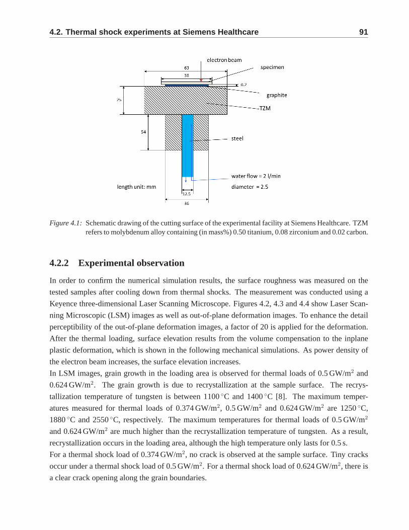
4.2. Thermal shock experiments at Siemens Healthcare 91
Figure 4.1: Schematic drawing of the cutting surface of the experimental facility at SiemensHealthcare. TZMrefers to molybdenum alloy containing (in mass%) 0.50 titanium, 0.08 zirconium and 0.02 carbon.
4.2.2 Experimental observation
In order to confirm the numerical simulation results, the surface roughness was measured on the
tested samples after cooling down from thermal shocks. The measurement was conducted using a
Keyence three-dimensional Laser Scanning Microscope. Figures 4.2, 4.3 and 4.4 show Laser Scan-
ning Microscopic (LSM) images as well as out-of-plane deformation images. To enhance the detail
perceptibility of the out-of-plane deformation images, a factor of 20 is applied for the deformation.
After the thermal loading, surface elevation results from the volume compensation to the inplane
plastic deformation, which is shown in the following mechanical simulations. As power density of
the electron beam increases, the surface elevation increases.
In LSM images, grain growth in the loading area is observed for thermal loads of 0.5 GW/m2 and
0.624 GW/m2. The grain growth is due to recrystallization at the sample surface. The recrys-
tallization temperature of tungsten is between 1100◦C and 1400◦C [8]. The maximum temper-
atures measured for thermal loads of 0.374 GW/m2, 0.5 GW/m2 and 0.624 GW/m2 are 1250◦C,
1880◦C and 2550◦C, respectively. The maximum temperatures for thermal loadsof 0.5 GW/m2
and 0.624 GW/m2 are much higher than the recrystallization temperature of tungsten. As a result,
recrystallization occurs in the loading area, although thehigh temperature only lasts for 0.5 s.
For a thermal shock load of 0.374 GW/m2, no crack is observed at the sample surface. Tiny cracks
occur under a thermal shock load of 0.5 GW/m2. For a thermal shock load of 0.624 GW/m2, there is
a clear crack opening along the grain boundaries.
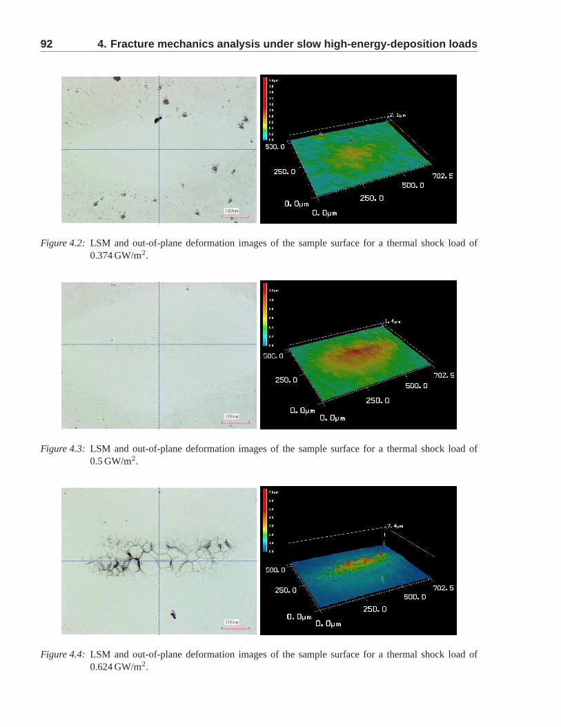
92 4. Fracture mechanics analysis under slow high-energy-d eposition loads
Figure 4.2: LSM and out-of-plane deformation images of the sample surface for a thermal shock load of0.374 GW/m2.
Figure 4.3: LSM and out-of-plane deformation images of the sample surface for a thermal shock load of0.5 GW/m2.
Figure 4.4: LSM and out-of-plane deformation images of the sample surface for a thermal shock load of0.624 GW/m2.
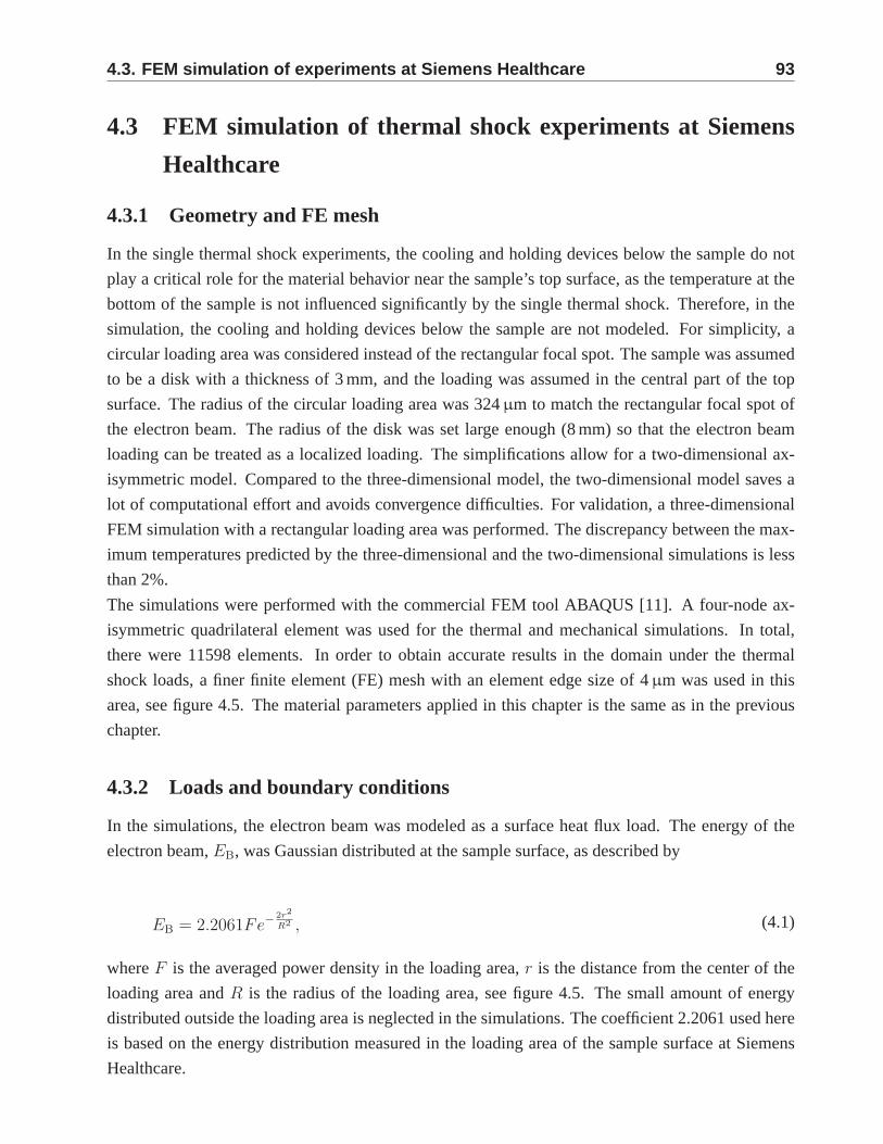
4.3. FEM simulation of experiments at Siemens Healthcare 93
4.3 FEM simulation of thermal shock experiments at Siemens
Healthcare
4.3.1 Geometry and FE mesh
In the single thermal shock experiments, the cooling and holding devices below the sample do not
play a critical role for the material behavior near the sample’s top surface, as the temperature at the
bottom of the sample is not influenced significantly by the single thermal shock. Therefore, in the
simulation, the cooling and holding devices below the sample are not modeled. For simplicity, a
circular loading area was considered instead of the rectangular focal spot. The sample was assumed
to be a disk with a thickness of 3 mm, and the loading was assumed in the central part of the top
surface. The radius of the circular loading area was 324µm to match the rectangular focal spot of
the electron beam. The radius of the disk was set large enough(8 mm) so that the electron beam
loading can be treated as a localized loading. The simplifications allow for a two-dimensional ax-
isymmetric model. Compared to the three-dimensional model,the two-dimensional model saves a
lot of computational effort and avoids convergence difficulties. For validation, a three-dimensional
FEM simulation with a rectangular loading area was performed. The discrepancy between the max-
imum temperatures predicted by the three-dimensional and the two-dimensional simulations is less
than 2%.
The simulations were performed with the commercial FEM toolABAQUS [11]. A four-node ax-
isymmetric quadrilateral element was used for the thermal and mechanical simulations. In total,
there were 11598 elements. In order to obtain accurate results in the domain under the thermal
shock loads, a finer finite element (FE) mesh with an element edge size of 4µm was used in this
area, see figure 4.5. The material parameters applied in thischapter is the same as in the previous
chapter.
4.3.2 Loads and boundary conditions
In the simulations, the electron beam was modeled as a surface heat flux load. The energy of the
electron beam,EB, was Gaussian distributed at the sample surface, as described by
EB = 2.2061Fe−2r
2
R2 , (4.1)
whereF is the averaged power density in the loading area,r is the distance from the center of the
loading area andR is the radius of the loading area, see figure 4.5. The small amount of energy
distributed outside the loading area is neglected in the simulations. The coefficient 2.2061 used here
is based on the energy distribution measured in the loading area of the sample surface at Siemens
Healthcare.
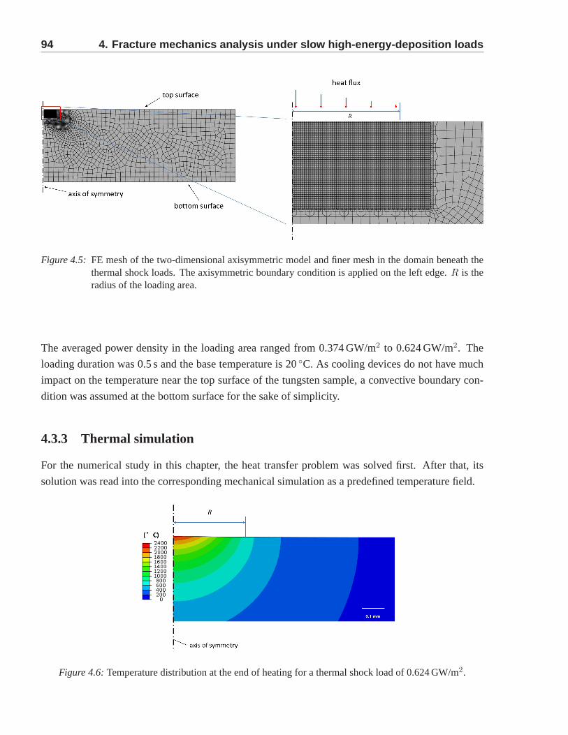
94 4. Fracture mechanics analysis under slow high-energy-d eposition loads
Figure 4.5: FE mesh of the two-dimensional axisymmetric model and finer mesh in the domain beneath thethermal shock loads. The axisymmetric boundary condition is applied on the left edge.R is theradius of the loading area.
The averaged power density in the loading area ranged from 0.374 GW/m2 to 0.624 GW/m2. The
loading duration was 0.5 s and the base temperature is 20◦C. As cooling devices do not have much
impact on the temperature near the top surface of the tungsten sample, a convective boundary con-
dition was assumed at the bottom surface for the sake of simplicity.
4.3.3 Thermal simulation
For the numerical study in this chapter, the heat transfer problem was solved first. After that, its
solution was read into the corresponding mechanical simulation as a predefined temperature field.
Figure 4.6: Temperature distribution at the end of heating for a thermal shock load of 0.624 GW/m2.
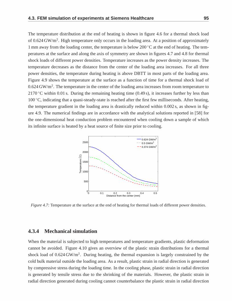
4.3. FEM simulation of experiments at Siemens Healthcare 95
The temperature distribution at the end of heating is shown in figure 4.6 for a thermal shock load
of 0.624 GW/m2. High temperature only occurs in the loading area. At a position of approximately
1 mm away from the loading center, the temperature is below 200 ◦C at the end of heating. The tem-
peratures at the surface and along the axis of symmetry are shown in figures 4.7 and 4.8 for thermal
shock loads of different power densities. Temperature increases as the power density increases. The
temperature decreases as the distance from the center of theloading area increases. For all three
power densities, the temperature during heating is above DBTT in most parts of the loading area.
Figure 4.9 shows the temperature at the surface as a functionof time for a thermal shock load of
0.624 GW/m2. The temperature in the center of the loading area increasesfrom room temperature to
2170◦C within 0.01 s. During the remaining heating time (0.49 s), it increases further by less than
100◦C, indicating that a quasi-steady-state is reached after thefirst few milliseconds. After heating,
the temperature gradient in the loading area is drasticallyreduced within 0.002 s, as shown in fig-
ure 4.9. The numerical findings are in accordance with the analytical solutions reported in [58] for
the one-dimensional heat conduction problem encountered when cooling down a sample of which
its infinite surface is heated by a heat source of finite size prior to cooling.
0 0.1 0.2 0.3 0.4 0.50
500
1000
1500
2000
2500
Distance from the center (mm)
Tem
pera
ture
(° C)
0.624 GW/m2
0.5 GW/m2
0.374 GW/m2
Figure 4.7: Temperature at the surface at the end of heating for thermal loads of different power densities.
4.3.4 Mechanical simulation
When the material is subjected to high temperatures and temperature gradients, plastic deformation
cannot be avoided. Figure 4.10 gives an overview of the plastic strain distributions for a thermal
shock load of 0.624 GW/m2. During heating, the thermal expansion is largely constrained by the
cold bulk material outside the loading area. As a result, plastic strain in radial direction is generated
by compressive stress during the loading time. In the cooling phase, plastic strain in radial direction
is generated by tensile stress due to the shrinking of the materials. However, the plastic strain in
radial direction generated during cooling cannot counterbalance the plastic strain in radial direction
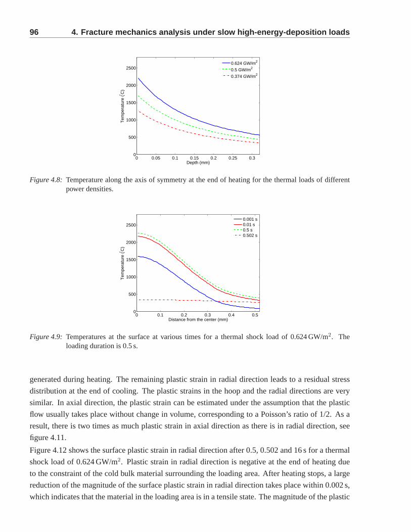
96 4. Fracture mechanics analysis under slow high-energy-d eposition loads
0 0.05 0.1 0.15 0.2 0.25 0.30
500
1000
1500
2000
2500
Depth (mm)
Tem
pera
ture
(° C)
0.624 GW/m2
0.5 GW/m2
0.374 GW/m2
Figure 4.8: Temperature along the axis of symmetry at the end of heating for the thermal loads of differentpower densities.
0 0.1 0.2 0.3 0.4 0.50
500
1000
1500
2000
2500
Distance from the center (mm)
Tem
pera
ture
(° C)
0.001 s0.01 s0.5 s0.502 s
Figure 4.9: Temperatures at the surface at various times for a thermal shock load of 0.624 GW/m2. Theloading duration is 0.5 s.
generated during heating. The remaining plastic strain in radial direction leads to a residual stress
distribution at the end of cooling. The plastic strains in the hoop and the radial directions are very
similar. In axial direction, the plastic strain can be estimated under the assumption that the plastic
flow usually takes place without change in volume, corresponding to a Poisson’s ratio of 1/2. As a
result, there is two times as much plastic strain in axial direction as there is in radial direction, see
figure 4.11.
Figure 4.12 shows the surface plastic strain in radial direction after 0.5, 0.502 and 16 s for a thermal
shock load of 0.624 GW/m2. Plastic strain in radial direction is negative at the end ofheating due
to the constraint of the cold bulk material surrounding the loading area. After heating stops, a large
reduction of the magnitude of the surface plastic strain in radial direction takes place within 0.002 s,
which indicates that the material in the loading area is in a tensile state. The magnitude of the plastic
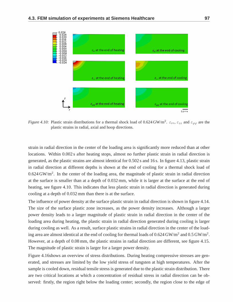
4.3. FEM simulation of experiments at Siemens Healthcare 97
Figure 4.10: Plastic strain distributions for a thermal shock load of 0.624 GW/m2. εrr, εzz andεϕϕ are theplastic strains in radial, axial and hoop directions.
strain in radial direction in the center of the loading area is significantly more reduced than at other
locations. Within 0.002 s after heating stops, almost no further plastic strain in radial direction is
generated, as the plastic strains are almost identical for 0.502 s and 16 s. In figure 4.13, plastic strain
in radial direction at different depths is shown at the end ofcooling for a thermal shock load of
0.624 GW/m2. In the center of the loading area, the magnitude of plastic strain in radial direction
at the surface is smaller than at a depth of 0.032 mm, while it is larger at the surface at the end of
heating, see figure 4.10. This indicates that less plastic strain in radial direction is generated during
cooling at a depth of 0.032 mm than there is at the surface.
The influence of power density at the surface plastic strain in radial direction is shown in figure 4.14.
The size of the surface plastic zone increases, as the power density increases. Although a larger
power density leads to a larger magnitude of plastic strain in radial direction in the center of the
loading area during heating, the plastic strain in radial direction generated during cooling is larger
during cooling as well. As a result, surface plastic strainsin radial direction in the center of the load-
ing area are almost identical at the end of cooling for thermal loads of 0.624 GW/m2 and 0.5 GW/m2.
However, at a depth of 0.08 mm, the plastic strains in radial direction are different, see figure 4.15.
The magnitude of plastic strain is larger for a larger power density.
Figure 4.16shows an overview of stress distributions. During heating compressive stresses are gen-
erated, and stresses are limited by the low yield stress of tungsten at high temperatures. After the
sample is cooled down, residual tensile stress is generateddue to the plastic strain distribution. There
are two critical locations at which a concentration of residual stress in radial direction can be ob-
served: firstly, the region right below the loading center; secondly, the region close to the edge of
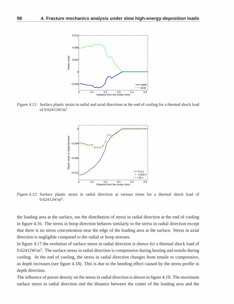
98 4. Fracture mechanics analysis under slow high-energy-d eposition loads
0 0.1 0.2 0.3 0.4 0.5
−0.004
0
0.004
0.008
0.012
Distance from the center (mm)
Pla
stic
str
ain
radialaxial
Figure 4.11: Surface plastic strain in radial and axial directions at the end of cooling for a thermal shock loadof 0.624 GW/m2
0 0.1 0.2 0.3 0.4 0.5
−0.012
−0.008
−0.004
0
Distance from the center (mm)
Pla
stic
str
ain
in r
adia
l dire
ctio
n
0.5 s0.502 s16 s
Figure 4.12: Surface plastic strain in radial direction at various times for a thermal shockload of0.624 GW/m2.
the loading area at the surface, see the distribution of stress in radial direction at the end of cooling
in figure 4.16. The stress in hoop direction behaves similarly to the stress in radial direction except
that there is no stress concentration near the edge of the loading area at the surface. Stress in axial
direction is negligible compared to the radial or hoop stresses.
In figure 4.17 the evolution of surface stress in radial direction is shown for a thermal shock load of
0.624 GW/m2. The surface stress in radial direction is compressive during heating and tensile during
cooling. At the end of cooling, the stress in radial direction changes from tensile to compressive,
as depth increases (see figure 4.18). This is due to the bending effect caused by the stress profile in
depth direction.
The influence of power density on the stress in radial direction is shown in figure 4.19. The maximum
surface stress in radial direction and the distance betweenthe center of the loading area and the
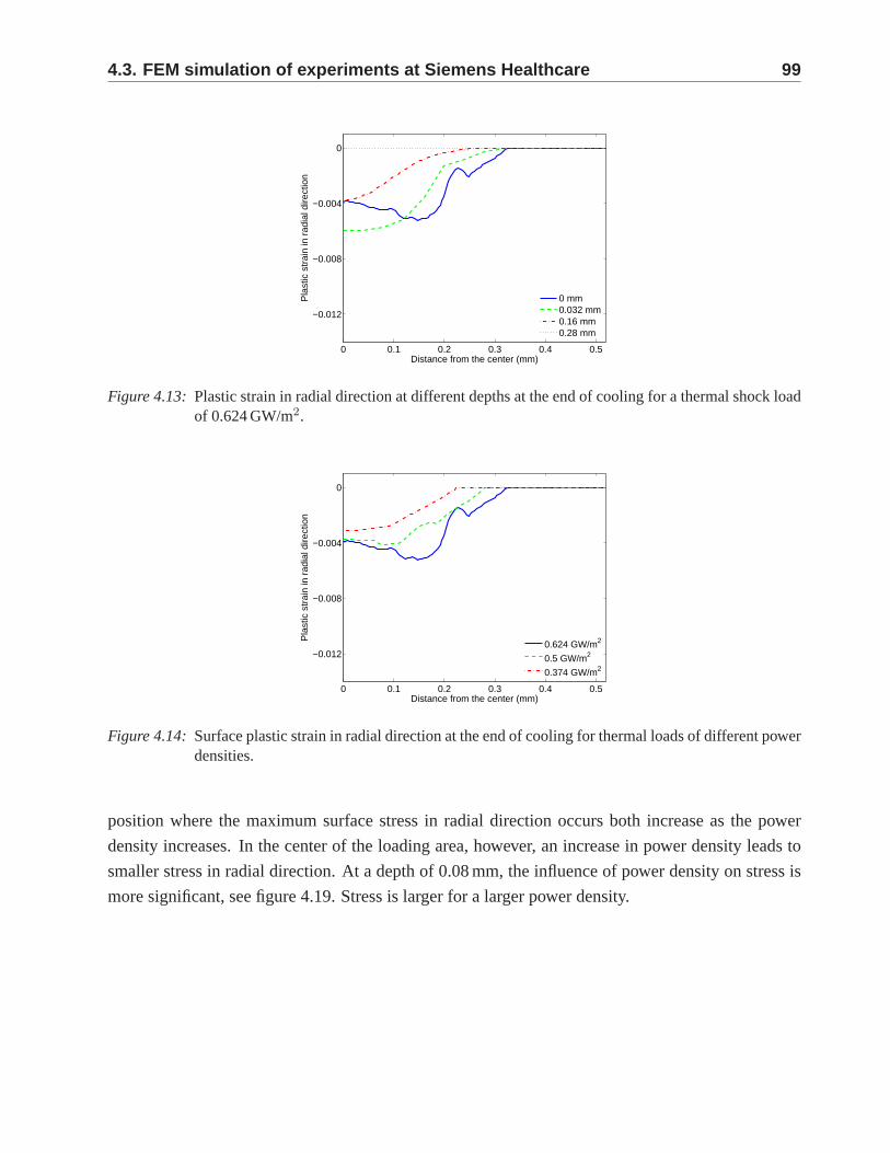
4.3. FEM simulation of experiments at Siemens Healthcare 99
0 0.1 0.2 0.3 0.4 0.5
−0.012
−0.008
−0.004
0
Distance from the center (mm)
Pla
stic
str
ain
in r
adia
l dire
ctio
n
0 mm0.032 mm0.16 mm0.28 mm
Figure 4.13: Plastic strain in radial direction at different depths at the end of cooling for a thermal shock loadof 0.624 GW/m2.
0 0.1 0.2 0.3 0.4 0.5
−0.012
−0.008
−0.004
0
Distance from the center (mm)
Pla
stic
str
ain
in r
adia
l dire
ctio
n
0.624 GW/m2
0.5 GW/m2
0.374 GW/m2
Figure 4.14: Surface plastic strain in radial direction at the end of cooling for thermal loads of different powerdensities.
position where the maximum surface stress in radial direction occurs both increase as the power
density increases. In the center of the loading area, however, an increase in power density leads to
smaller stress in radial direction. At a depth of 0.08 mm, theinfluence of power density on stress is
more significant, see figure 4.19. Stress is larger for a larger power density.
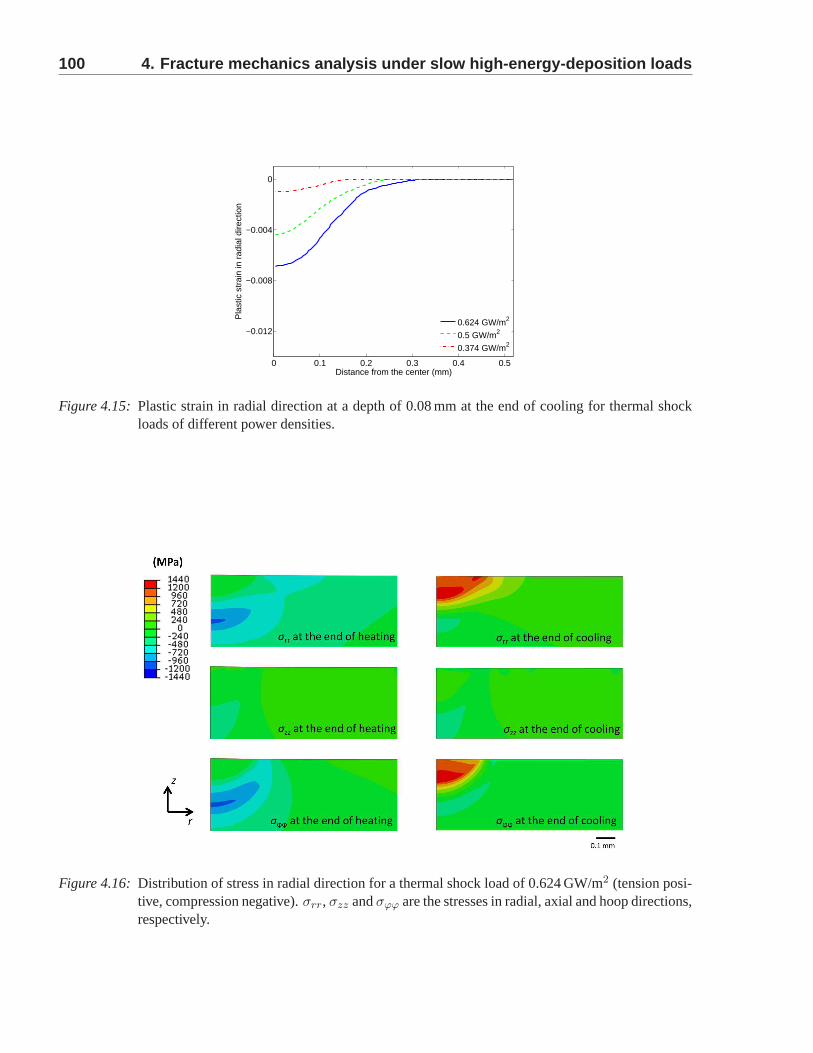
100 4. Fracture mechanics analysis under slow high-energy- deposition loads
0 0.1 0.2 0.3 0.4 0.5
−0.012
−0.008
−0.004
0
Distance from the center (mm)
Pla
stic
str
ain
in r
adia
l dire
ctio
n
0.624 GW/m2
0.5 GW/m2
0.374 GW/m2
Figure 4.15: Plastic strain in radial direction at a depth of 0.08 mm at the end of cooling for thermal shockloads of different power densities.
Figure 4.16: Distribution of stress in radial direction for a thermal shock load of 0.624 GW/m2 (tension posi-tive, compression negative).σrr, σzz andσϕϕ are the stresses in radial, axial and hoop directions,respectively.
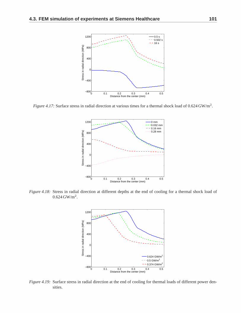
4.3. FEM simulation of experiments at Siemens Healthcare 101
0 0.1 0.2 0.3 0.4 0.5−800
−400
0
400
800
1200
Distance from the center (mm)
Str
ess
in r
adia
l dire
ctio
n (M
Pa)
0.5 s0.502 s16 s
Figure 4.17: Surface stress in radial direction at various times for a thermal shock loadof 0.624 GW/m2.
0 0.1 0.2 0.3 0.4 0.5−800
−400
0
400
800
1200
Distance from the center (mm)
Str
ess
in r
adia
l dire
ctio
n (M
Pa)
0 mm0.032 mm0.16 mm0.28 mm
Figure 4.18: Stress in radial direction at different depths at the end of cooling for a thermal shock load of0.624 GW/m2.
0 0.1 0.2 0.3 0.4 0.5−800
−400
0
400
800
1200
Distance from the center (mm)
Str
ess
in r
adia
l dire
ctio
n (M
Pa)
0.624 GW/m2
0.5 GW/m2
0.374 GW/m2
Figure 4.19: Surface stress in radial direction at the end of cooling for thermal loads of different power den-sities.
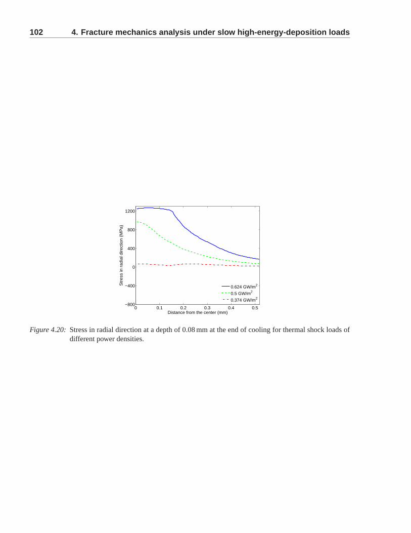
102 4. Fracture mechanics analysis under slow high-energy- deposition loads
0 0.1 0.2 0.3 0.4 0.5−800
−400
0
400
800
1200
Distance from the center (mm)
Str
ess
in r
adia
l dire
ctio
n (M
Pa)
0.624 GW/m2
0.5 GW/m2
0.374 GW/m2
Figure 4.20: Stress in radial direction at a depth of 0.08 mm at the end of cooling for thermal shock loads ofdifferent power densities.
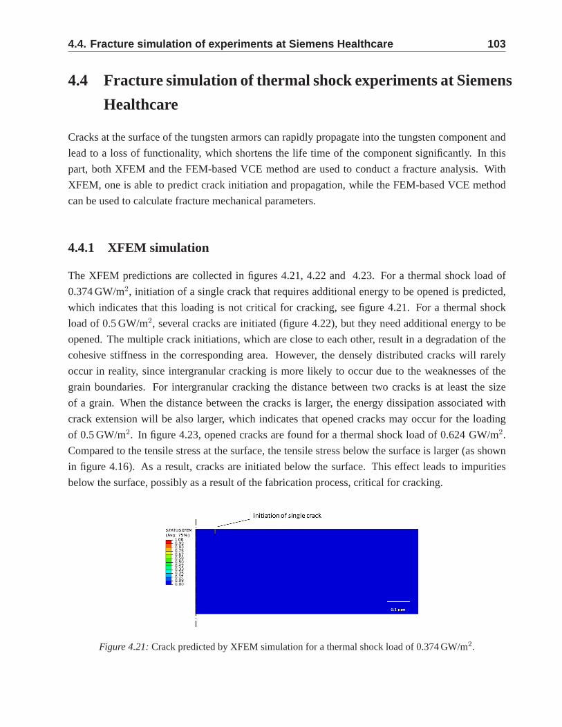
4.4. Fracture simulation of experiments at Siemens Healthca re 103
4.4 Fracture simulation of thermal shock experiments at Siemens
Healthcare
Cracks at the surface of the tungsten armors can rapidly propagate into the tungsten component and
lead to a loss of functionality, which shortens the life timeof the component significantly. In this
part, both XFEM and the FEM-based VCE method are used to conduct a fracture analysis. With
XFEM, one is able to predict crack initiation and propagation, while the FEM-based VCE method
can be used to calculate fracture mechanical parameters.
4.4.1 XFEM simulation
The XFEM predictions are collected in figures 4.21, 4.22 and 4.23. For a thermal shock load of
0.374 GW/m2, initiation of a single crack that requires additional energy to be opened is predicted,
which indicates that this loading is not critical for cracking, see figure 4.21. For a thermal shock
load of 0.5 GW/m2, several cracks are initiated (figure 4.22), but they need additional energy to be
opened. The multiple crack initiations, which are close to each other, result in a degradation of the
cohesive stiffness in the corresponding area. However, thedensely distributed cracks will rarely
occur in reality, since intergranular cracking is more likely to occur due to the weaknesses of the
grain boundaries. For intergranular cracking the distancebetween two cracks is at least the size
of a grain. When the distance between the cracks is larger, theenergy dissipation associated with
crack extension will be also larger, which indicates that opened cracks may occur for the loading
of 0.5 GW/m2. In figure 4.23, opened cracks are found for a thermal shock load of 0.624 GW/m2.
Compared to the tensile stress at the surface, the tensile stress below the surface is larger (as shown
in figure 4.16). As a result, cracks are initiated below the surface. This effect leads to impurities
below the surface, possibly as a result of the fabrication process, critical for cracking.
Figure 4.21: Crack predicted by XFEM simulation for a thermal shock load of 0.374 GW/m2.
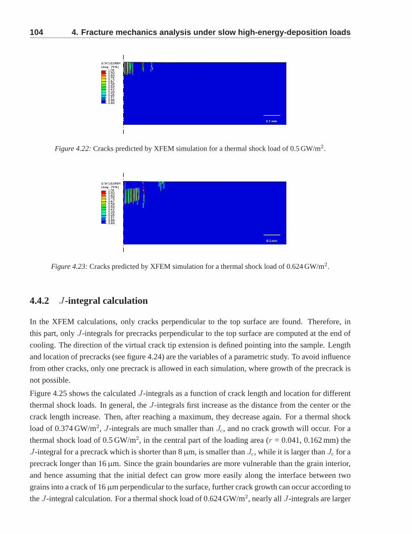
104 4. Fracture mechanics analysis under slow high-energy- deposition loads
Figure 4.22: Cracks predicted by XFEM simulation for a thermal shock load of 0.5 GW/m2.
Figure 4.23: Cracks predicted by XFEM simulation for a thermal shock load of 0.624 GW/m2.
4.4.2 J-integral calculation
In the XFEM calculations, only cracks perpendicular to the top surface are found. Therefore, in
this part, onlyJ-integrals for precracks perpendicular to the top surface are computed at the end of
cooling. The direction of the virtual crack tip extension isdefined pointing into the sample. Length
and location of precracks (see figure 4.24) are the variablesof a parametric study. To avoid influence
from other cracks, only one precrack is allowed in each simulation, where growth of the precrack is
not possible.
Figure 4.25 shows the calculatedJ-integrals as a function of crack length and location for different
thermal shock loads. In general, theJ-integrals first increase as the distance from the center or the
crack length increase. Then, after reaching a maximum, theydecrease again. For a thermal shock
load of 0.374 GW/m2, J-integrals are much smaller thanJc, and no crack growth will occur. For a
thermal shock load of 0.5 GW/m2, in the central part of the loading area (r = 0.041, 0.162 mm) the
J-integral for a precrack which is shorter than 8µm, is smaller thanJc, while it is larger thanJc for a
precrack longer than 16µm. Since the grain boundaries are more vulnerable than the grain interior,
and hence assuming that the initial defect can grow more easily along the interface between two
grains into a crack of 16µm perpendicular to the surface, further crack growth can occur according to
theJ-integral calculation. For a thermal shock load of 0.624 GW/m2, nearly allJ-integrals are larger
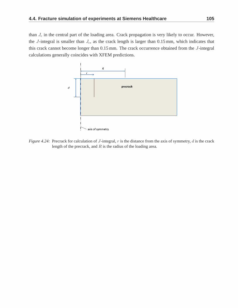
4.4. Fracture simulation of experiments at Siemens Healthca re 105
thanJc in the central part of the loading area. Crack propagation is very likely to occur. However,
the J-integral is smaller thanJc, as the crack length is larger than 0.15 mm, which indicates that
this crack cannot become longer than 0.15 mm. The crack occurrence obtained from theJ-integral
calculations generally coincides with XFEM predictions.
Figure 4.24: Precrack for calculation ofJ-integral,r is the distance from the axis of symmetry,d is the cracklength of the precrack, andR is the radius of the loading area.
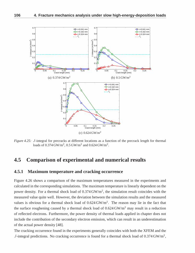
106 4. Fracture mechanics analysis under slow high-energy- deposition loads
0 0.05 0.1 0.15 0.2 0.250
0.1
0.2
0.3
0.4
0.5
0.6
0.7
Crack length (mm)
J−in
tegr
al (
mJ/
mm
2 )
r=0.041 mmr=0.162 mmr=0.324 mmJ
c
(a) 0.374 GW/m2
0 0.05 0.1 0.15 0.2 0.250
0.1
0.2
0.3
0.4
0.5
0.6
0.7
Crack length (mm)
J−in
tegr
al (
mJ/
mm
2 )
r=0.041 mmr=0.162 mmr=0.324 mmJ
c
(b) 0.5 GW/m2
0 0.05 0.1 0.15 0.2 0.250
0.1
0.2
0.3
0.4
0.5
0.6
0.7
Crack length (mm)
J−in
tegr
al (
mJ/
mm
2 )
r=0.041 mmr=0.162 mmr=0.324 mmJ
c
(c) 0.624 GW/m2
Figure 4.25: J-integral for precracks at different locations as a function of the precrack length for thermalloads of 0.374 GW/m2, 0.5 GW/m2 and 0.624 GW/m2.
4.5 Comparison of experimental and numerical results
4.5.1 Maximum temperature and cracking occurrence
Figure 4.26 shows a comparison of the maximum temperatures measured in the experiments and
calculated in the corresponding simulations. The maximum temperature is linearly dependent on the
power density. For a thermal shock load of 0.374 GW/m2, the simulation result coincides with the
measured value quite well. However, the deviation between the simulation results and the measured
values is obvious for a thermal shock load of 0.624 GW/m2. The reason may lie in the fact that
the surface roughening caused by a thermal shock load of 0.624 GW/m2 may result in a reduction
of reflected electrons. Furthermore, the power density of thermal loads applied in chapter does not
include the contribution of the secondary electron emission, which can result in an underestimation
of the actual power density [48].
The cracking occurrence found in the experiments generallycoincides with both the XFEM and the
J-integral predictions. No cracking occurrence is found fora thermal shock load of 0.374 GW/m2,
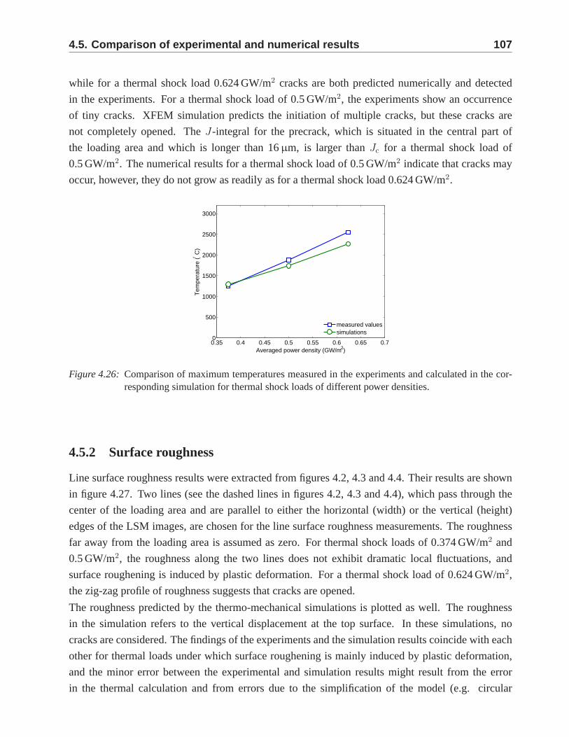
4.5. Comparison of experimental and numerical results 107
while for a thermal shock load 0.624 GW/m2 cracks are both predicted numerically and detected
in the experiments. For a thermal shock load of 0.5 GW/m2, the experiments show an occurrence
of tiny cracks. XFEM simulation predicts the initiation of multiple cracks, but these cracks are
not completely opened. TheJ-integral for the precrack, which is situated in the centralpart of
the loading area and which is longer than 16µm, is larger thanJc for a thermal shock load of
0.5 GW/m2. The numerical results for a thermal shock load of 0.5 GW/m2 indicate that cracks may
occur, however, they do not grow as readily as for a thermal shock load 0.624 GW/m2.
0.35 0.4 0.45 0.5 0.55 0.6 0.65 0.70
500
1000
1500
2000
2500
3000
Averaged power density (GW/m2)
Tem
pera
ture
(° C)
measured valuessimulations
Figure 4.26: Comparison of maximum temperatures measured in the experiments and calculatedin the cor-responding simulation for thermal shock loads of different power densities.
4.5.2 Surface roughness
Line surface roughness results were extracted from figures 4.2, 4.3 and 4.4. Their results are shown
in figure 4.27. Two lines (see the dashed lines in figures 4.2, 4.3 and 4.4), which pass through the
center of the loading area and are parallel to either the horizontal (width) or the vertical (height)
edges of the LSM images, are chosen for the line surface roughness measurements. The roughness
far away from the loading area is assumed as zero. For thermalshock loads of 0.374 GW/m2 and
0.5 GW/m2, the roughness along the two lines does not exhibit dramaticlocal fluctuations, and
surface roughening is induced by plastic deformation. For athermal shock load of 0.624 GW/m2,
the zig-zag profile of roughness suggests that cracks are opened.
The roughness predicted by the thermo-mechanical simulations is plotted as well. The roughness
in the simulation refers to the vertical displacement at thetop surface. In these simulations, no
cracks are considered. The findings of the experiments and the simulation results coincide with each
other for thermal loads under which surface roughening is mainly induced by plastic deformation,
and the minor error between the experimental and simulationresults might result from the error
in the thermal calculation and from errors due to the simplification of the model (e.g. circular

108 4. Fracture mechanics analysis under slow high-energy- deposition loads
−400 −300 −200 −100 0 100 200 300 4000
0.5
1
1.5
2
2.5
3
3.5
4
Width or height (µm)
Rou
ghne
ss (
µm)
WidthHeightSimulated
(a) 0.374 GW/m2
−400 −300 −200 −100 0 100 200 300 4000
0.5
1
1.5
2
2.5
3
3.5
4
Width or height (µm)
Rou
ghne
ss (
µm)
WidthHeightSimulated
(b) 0.5 GW/m2
−400 −300 −200 −100 0 100 200 300 4000
0.5
1
1.5
2
2.5
3
3.5
4
Width or height (µm)
Rou
ghne
ss (
µm)
WidthHeightSimulated
(c) 0.624 GW/m2
Figure 4.27: Roughness for thermal shock loads of 0.374 GW/m2, 0.5 GW/m2 and 0.624 GW/m2. Width:measured roughness along the horizontal dashed lines in figures 4.2, 4.3and 4.4, Height: mea-sured roughness along the vertical dashed lines in the same figures, Simulated: surface verticaldisplacement in the simulations.
instead of rectangular loading area). If cracks are opened,there are obvious differences between the
experimental and the simulation results, see figure 4.27 c.
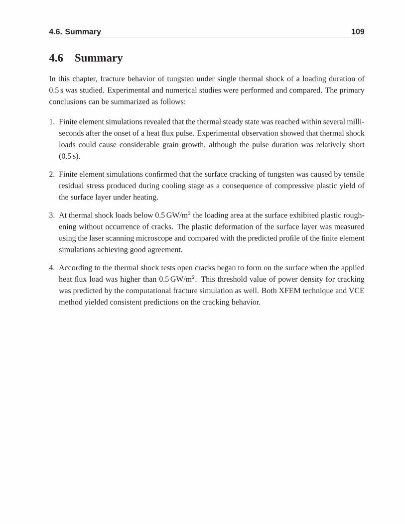
4.6. Summary 109
4.6 Summary
In this chapter, fracture behavior of tungsten under singlethermal shock of a loading duration of
0.5 s was studied. Experimental and numerical studies were performed and compared. The primary
conclusions can be summarized as follows:
1. Finite element simulations revealed that the thermal steady state was reached within several milli-
seconds after the onset of a heat flux pulse. Experimental observation showed that thermal shock
loads could cause considerable grain growth, although the pulse duration was relatively short
(0.5 s).
2. Finite element simulations confirmed that the surface cracking of tungsten was caused by tensile
residual stress produced during cooling stage as a consequence of compressive plastic yield of
the surface layer under heating.
3. At thermal shock loads below 0.5 GW/m2 the loading area at the surface exhibited plastic rough-
ening without occurrence of cracks. The plastic deformation of the surface layer was measured
using the laser scanning microscope and compared with the predicted profile of the finite element
simulations achieving good agreement.
4. According to the thermal shock tests open cracks began to form on the surface when the applied
heat flux load was higher than 0.5 GW/m2. This threshold value of power density for cracking
was predicted by the computational fracture simulation as well. Both XFEM technique and VCE
method yielded consistent predictions on the cracking behavior.
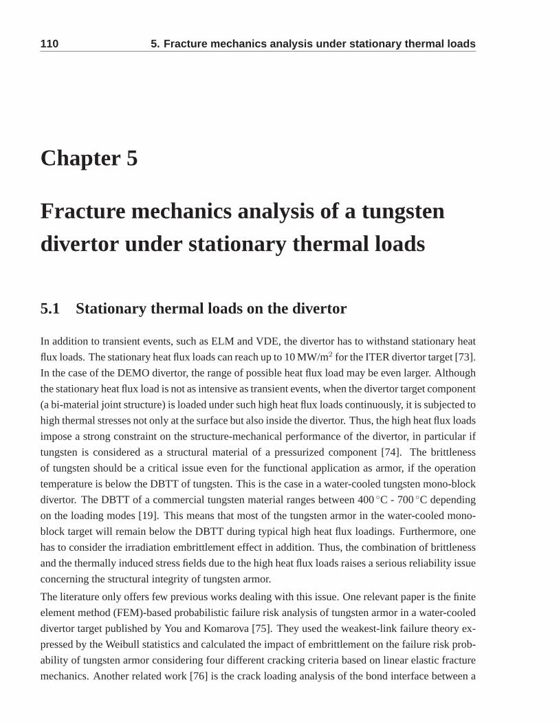
110 5. Fracture mechanics analysis under stationary therma l loads
Chapter 5
Fracture mechanics analysis of a tungsten
divertor under stationary thermal loads
5.1 Stationary thermal loads on the divertor
In addition to transient events, such as ELM and VDE, the divertor has to withstand stationary heat
flux loads. The stationary heat flux loads can reach up to 10 MW/m2 for the ITER divertor target [73].
In the case of the DEMO divertor, the range of possible heat flux load may be even larger. Although
the stationary heat flux load is not as intensive as transientevents, when the divertor target component
(a bi-material joint structure) is loaded under such high heat flux loads continuously, it is subjected to
high thermal stresses not only at the surface but also insidethe divertor. Thus, the high heat flux loads
impose a strong constraint on the structure-mechanical performance of the divertor, in particular if
tungsten is considered as a structural material of a pressurized component [74]. The brittleness
of tungsten should be a critical issue even for the functional application as armor, if the operation
temperature is below the DBTT of tungsten. This is the case in awater-cooled tungsten mono-block
divertor. The DBTT of a commercial tungsten material ranges between 400◦C - 700◦C depending
on the loading modes [19]. This means that most of the tungsten armor in the water-cooled mono-
block target will remain below the DBTT during typical high heat flux loadings. Furthermore, one
has to consider the irradiation embrittlement effect in addition. Thus, the combination of brittleness
and the thermally induced stress fields due to the high heat flux loads raises a serious reliability issue
concerning the structural integrity of tungsten armor.
The literature only offers few previous works dealing with this issue. One relevant paper is the finite
element method (FEM)-based probabilistic failure risk analysis of tungsten armor in a water-cooled
divertor target published by You and Komarova [75]. They used the weakest-link failure theory ex-
pressed by the Weibull statistics and calculated the impactof embrittlement on the failure risk prob-
ability of tungsten armor considering four different cracking criteria based on linear elastic fracture
mechanics. Another related work [76] is the crack loading analysis of the bond interface between a
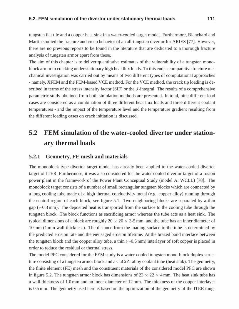
5.2. FEM simulation of the divertor under stationary thermal loads 111
tungsten flat tile and a copper heat sink in a water-cooled target model. Furthermore, Blanchard and
Martin studied the fracture and creep behavior of an all-tungsten divertor for ARIES [77]. However,
there are no previous reports to be found in the literature that are dedicated to a thorough fracture
analysis of tungsten armor apart from these.
The aim of this chapter is to deliver quantitative estimatesof the vulnerability of a tungsten mono-
block armor to cracking under stationary high heat flux loads. To this end, a comparative fracture me-
chanical investigation was carried out by means of two different types of computational approaches
- namely, XFEM and the FEM-based VCE method. For the VCE method,the crack tip loading is de-
scribed in terms of the stress intensity factor (SIF) or theJ-integral. The results of a comprehensive
parametric study obtained from both simulation methods arepresented. In total, nine different load
cases are considered as a combination of three different heat flux loads and three different coolant
temperatures - and the impact of the temperature level and the temperature gradient resulting from
the different loading cases on crack initiation is discussed.
5.2 FEM simulation of the water-cooled divertor under station-
ary thermal loads
5.2.1 Geometry, FE mesh and materials
The monoblock type divertor target model has already been applied to the water-cooled divertor
target of ITER. Furthermore, it was also considered for the water-cooled divertor target of a fusion
power plant in the framework of the Power Plant Conceptual Study (model A: WCLL) [78]. The
monoblock target consists of a number of small rectangular tungsten blocks which are connected by
a long cooling tube made of a high thermal conductivity metal(e.g. copper alloy) running through
the central region of each block, see figure 5.1. Two neighboring blocks are separated by a thin
gap (∼0.3 mm). The deposited heat is transported from the surface to the cooling tube through the
tungsten block. The block functions as sacrificing armor whereas the tube acts as a heat sink. The
typical dimensions of a block are roughly 20× 20 × 3-5 mm, and the tube has an inner diameter of
10 mm (1 mm wall thickness). The distance from the loading surface to the tube is determined by
the predicted erosion rate and the envisaged erosion lifetime. At the brazed bond interface between
the tungsten block and the copper alloy tube, a thin (∼0.5 mm) interlayer of soft copper is placed in
order to reduce the residual or thermal stress.
The model PFC considered for the FEM study is a water-cooled tungsten mono-block duplex struc-
ture consisting of a tungsten armor block and a CuCrZr alloy coolant tube (heat sink). The geometry,
the finite element (FE) mesh and the constituent materials ofthe considered model PFC are shown
in figure 5.2. The tungsten armor block has dimensions of 23× 22 × 4 mm. The heat sink tube has
a wall thickness of 1.0 mm and an inner diameter of 12 mm. The thickness of the copper interlayer
is 0.5 mm. The geometry used here is based on the optimizationof the geometry of the ITER tung-
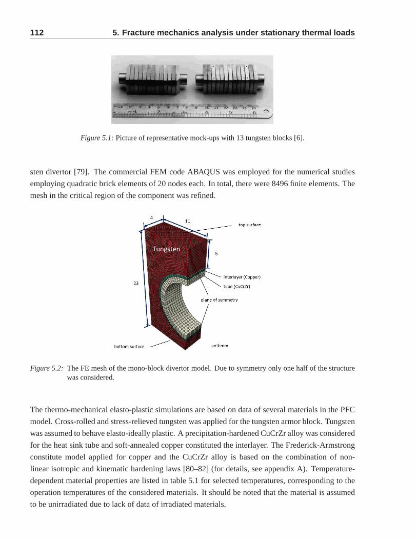
112 5. Fracture mechanics analysis under stationary therma l loads
Figure 5.1: Picture of representative mock-ups with 13 tungsten blocks [6].
sten divertor [79]. The commercial FEM code ABAQUS was employed for the numerical studies
employing quadratic brick elements of 20 nodes each. In total, there were 8496 finite elements. The
mesh in the critical region of the component was refined.
Figure 5.2: The FE mesh of the mono-block divertor model. Due to symmetry only one half ofthe structurewas considered.
The thermo-mechanical elasto-plastic simulations are based on data of several materials in the PFC
model. Cross-rolled and stress-relieved tungsten was applied for the tungsten armor block. Tungsten
was assumed to behave elasto-ideally plastic. A precipitation-hardened CuCrZr alloy was considered
for the heat sink tube and soft-annealed copper constitutedthe interlayer. The Frederick-Armstrong
constitute model applied for copper and the CuCrZr alloy is based on the combination of non-
linear isotropic and kinematic hardening laws [80–82] (fordetails, see appendix A). Temperature-
dependent material properties are listed in table 5.1 for selected temperatures, corresponding to the
operation temperatures of the considered materials. It should be noted that the material is assumed
to be unirradiated due to lack of data of irradiated materials.
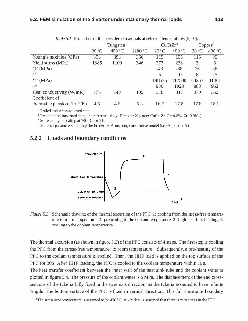
5.2. FEM simulation of the divertor under stationary thermal loads 113
Table 5.1: Properties of the considered materials at selected temperatures [9,10].
Tungsten1 CuCrZr2 Copper3
20◦C 400◦C 1200◦C 20◦C 400◦C 20◦C 400◦CYoung’s modulus (GPa) 398 393 356 115 106 115 95Yield stress (MPa) 1385 1100 346 273 238 3 3Q∗ (MPa) -43 -68 76 36b∗ 6 10 8 25C∗ (MPa) 148575 117500 64257 31461γ∗ 930 1023 888 952Heat conductivity (W/mK) 175 140 105 318 347 379 352Coefficient ofthermal expansion (10−6/K) 4.5 4.6 5.3 16.7 17.8 17.8 18.1
1 Rolled and stress-relieved state.2 Precipitation-hardened state, the reference alloy: Elmedur-X (code: CuCr1Zr, Cr: 0.8%, Zr: 0.08%).3 Softened by annealing at 700◦C for 1 h.∗ Material parameters entering the Frederick-Armstrong constitutive model (see Appendix A).
5.2.2 Loads and boundary conditions
Figure 5.3: Schematic drawing of the thermal excursion of the PFC. 1: cooling from the stress-free tempera-ture to room temperature, 2: preheating to the coolant temperature, 3: high heat flux loading, 4:cooling to the coolant temperature.
The thermal excursion (as shown in figure 5.3) of the PFC consists of 4 steps. The first step is cooling
the PFC from the stress-free temperature1 to room temperature. Subsequently, a pre-heating of the
PFC to the coolant temperature is applied. Then, the HHF loadis applied on the top surface of the
PFC for 30 s. After HHF loading, the PFC is cooled to the coolant temperature within 10 s.
The heat transfer coefficient between the inner wall of the heat sink tube and the coolant water is
plotted in figure 5.4. The pressure of the coolant water is 5 MPa. The displacement of the end cross-
sections of the tube is fully fixed in the tube axis direction,as the tube is assumed to have infinite
length. The bottom surface of the PFC is fixed in vertical direction. This full constraint boundary
1The stress-free temperature is assumed to be 450◦C, at which it is assumed that there is zero stress in the PFC.
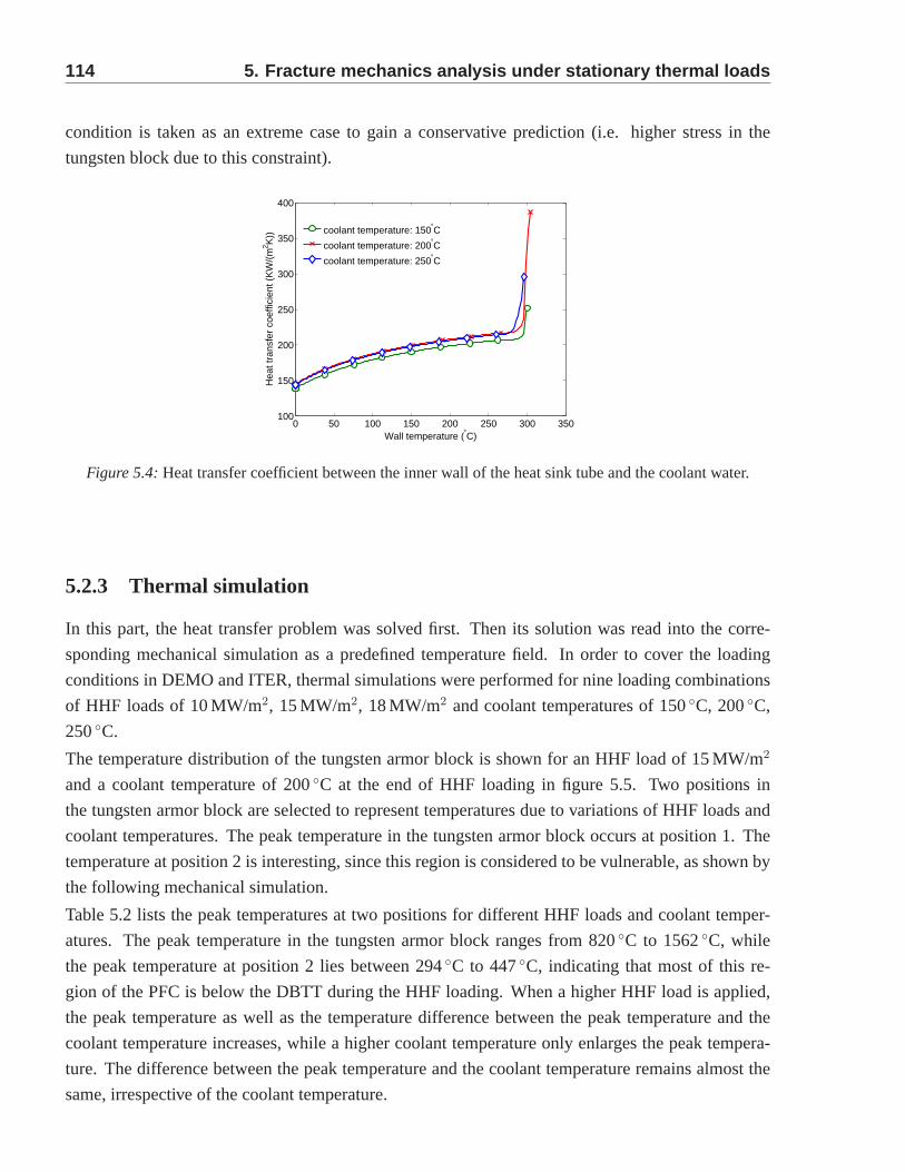
114 5. Fracture mechanics analysis under stationary therma l loads
condition is taken as an extreme case to gain a conservative prediction (i.e. higher stress in the
tungsten block due to this constraint).
0 50 100 150 200 250 300 350100
150
200
250
300
350
400
Wall temperature (°C)
Hea
t tra
nsfe
r co
effic
ient
(K
W/(
m2 K
))
coolant temperature: 150°C
coolant temperature: 200°C
coolant temperature: 250°C
Figure 5.4: Heat transfer coefficient between the inner wall of the heat sink tube and the coolant water.
5.2.3 Thermal simulation
In this part, the heat transfer problem was solved first. Thenits solution was read into the corre-
sponding mechanical simulation as a predefined temperaturefield. In order to cover the loading
conditions in DEMO and ITER, thermal simulations were performed for nine loading combinations
of HHF loads of 10 MW/m2, 15 MW/m2, 18 MW/m2 and coolant temperatures of 150◦C, 200◦C,
250◦C.
The temperature distribution of the tungsten armor block isshown for an HHF load of 15 MW/m2
and a coolant temperature of 200◦C at the end of HHF loading in figure 5.5. Two positions in
the tungsten armor block are selected to represent temperatures due to variations of HHF loads and
coolant temperatures. The peak temperature in the tungstenarmor block occurs at position 1. The
temperature at position 2 is interesting, since this regionis considered to be vulnerable, as shown by
the following mechanical simulation.
Table 5.2 lists the peak temperatures at two positions for different HHF loads and coolant temper-
atures. The peak temperature in the tungsten armor block ranges from 820◦C to 1562◦C, while
the peak temperature at position 2 lies between 294◦C to 447◦C, indicating that most of this re-
gion of the PFC is below the DBTT during the HHF loading. When a higher HHF load is applied,
the peak temperature as well as the temperature difference between the peak temperature and the
coolant temperature increases, while a higher coolant temperature only enlarges the peak tempera-
ture. The difference between the peak temperature and the coolant temperature remains almost the
same, irrespective of the coolant temperature.
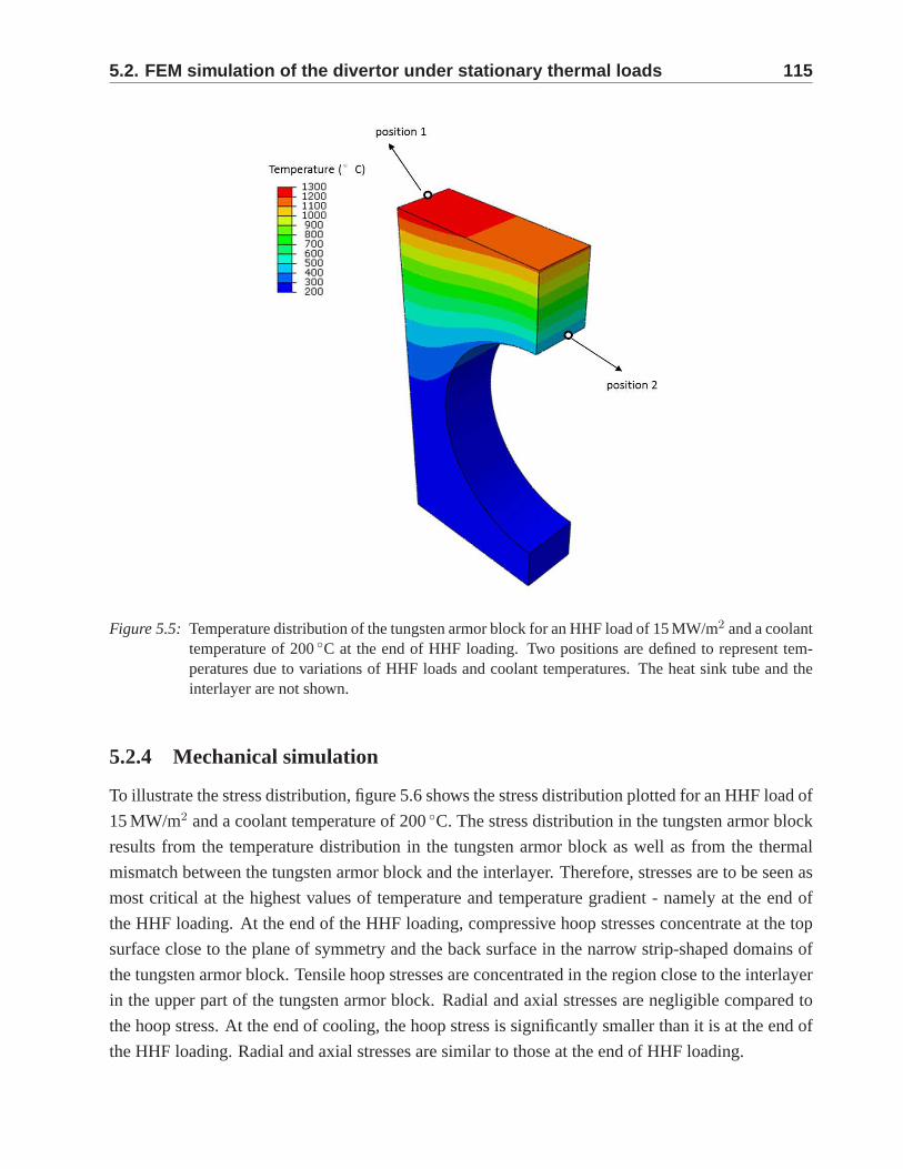
5.2. FEM simulation of the divertor under stationary thermal loads 115
Figure 5.5: Temperature distribution of the tungsten armor block for an HHF load of 15 MW/m2 and a coolanttemperature of 200◦C at the end of HHF loading. Two positions are defined to represent tem-peratures due to variations of HHF loads and coolant temperatures. The heat sink tube and theinterlayer are not shown.
5.2.4 Mechanical simulation
To illustrate the stress distribution, figure 5.6 shows the stress distribution plotted for an HHF load of
15 MW/m2 and a coolant temperature of 200◦C. The stress distribution in the tungsten armor block
results from the temperature distribution in the tungsten armor block as well as from the thermal
mismatch between the tungsten armor block and the interlayer. Therefore, stresses are to be seen as
most critical at the highest values of temperature and temperature gradient - namely at the end of
the HHF loading. At the end of the HHF loading, compressive hoop stresses concentrate at the top
surface close to the plane of symmetry and the back surface inthe narrow strip-shaped domains of
the tungsten armor block. Tensile hoop stresses are concentrated in the region close to the interlayer
in the upper part of the tungsten armor block. Radial and axialstresses are negligible compared to
the hoop stress. At the end of cooling, the hoop stress is significantly smaller than it is at the end of
the HHF loading. Radial and axial stresses are similar to those at the end of HHF loading.
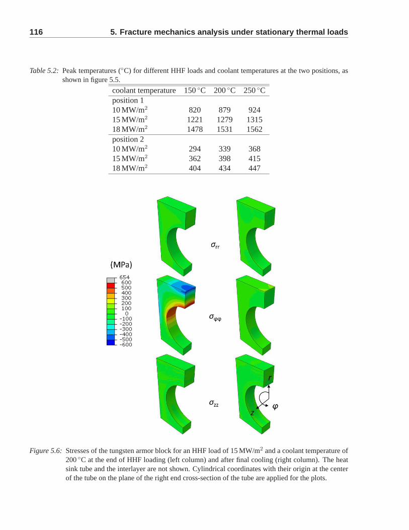
116 5. Fracture mechanics analysis under stationary therma l loads
Table 5.2: Peak temperatures (◦C) for different HHF loads and coolant temperatures at the two positions,asshown in figure 5.5.
coolant temperature 150◦C 200◦C 250◦Cposition 110 MW/m2 820 879 92415 MW/m2 1221 1279 131518 MW/m2 1478 1531 1562position 210 MW/m2 294 339 36815 MW/m2 362 398 41518 MW/m2 404 434 447
Figure 5.6: Stresses of the tungsten armor block for an HHF load of 15 MW/m2 and a coolant temperature of200◦C at the end of HHF loading (left column) and after final cooling (right column). The heatsink tube and the interlayer are not shown. Cylindrical coordinates with their origin at the centerof the tube on the plane of the right end cross-section of the tube are applied for the plots.
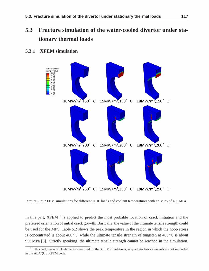
5.3. Fracture simulation of the divertor under stationary t hermal loads 117
5.3 Fracture simulation of the water-cooled divertor under sta-
tionary thermal loads
5.3.1 XFEM simulation
Figure 5.7: XFEM simulations for different HHF loads and coolant temperatures with an MPS of 400 MPa.
In this part, XFEM1 is applied to predict the most probable location of crack initiation and the
preferred orientation of initial crack growth. Basically, the value of the ultimate tensile strength could
be used for the MPS. Table 5.2 shows the peak temperature in the region in which the hoop stress
is concentrated is about 400◦C, while the ultimate tensile strength of tungsten at 400◦C is about
950 MPa [8]. Strictly speaking, the ultimate tensile strength cannot be reached in the simulation.
1In this part, linear brick elements were used for the XFEM simulations, as quadratic brick elements are not supportedin the ABAQUS XFEM code.
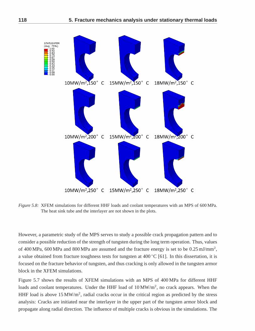
118 5. Fracture mechanics analysis under stationary therma l loads
Figure 5.8: XFEM simulations for different HHF loads and coolant temperatures with an MPS of 600 MPa.The heat sink tube and the interlayer are not shown in the plots.
However, a parametric study of the MPS serves to study a possible crack propagation pattern and to
consider a possible reduction of the strength of tungsten during the long term operation. Thus, values
of 400 MPa, 600 MPa and 800 MPa are assumed and the fracture energy is set to be 0.25 mJ/mm2,
a value obtained from fracture toughness tests for tungstenat 400◦C [61]. In this dissertation, it is
focused on the fracture behavior of tungsten, and thus cracking is only allowed in the tungsten armor
block in the XFEM simulations.
Figure 5.7 shows the results of XFEM simulations with an MPS of 400 MPa for different HHF
loads and coolant temperatures. Under the HHF load of 10 MW/m2, no crack appears. When the
HHF load is above 15 MW/m2, radial cracks occur in the critical region as predicted by the stress
analysis: Cracks are initiated near the interlayer in the upper part of the tungsten armor block and
propagate along radial direction. The influence of multiplecracks is obvious in the simulations. The
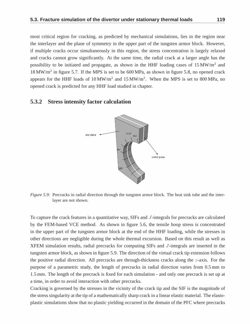
5.3. Fracture simulation of the divertor under stationary t hermal loads 119
most critical region for cracking, as predicted by mechanical simulations, lies in the region near
the interlayer and the plane of symmetry in the upper part of the tungsten armor block. However,
if multiple cracks occur simultaneously in this region, thestress concentration is largely relaxed
and cracks cannot grow significantly. At the same time, the radial crack at a larger angle has the
possibility to be initiated and propagate, as shown in the HHF loading cases of 15 MW/m2 and
18 MW/m2 in figure 5.7. If the MPS is set to be 600 MPa, as shown in figure 5.8, no opened crack
appears for the HHF loads of 10 MW/m2 and 15 MW/m2. When the MPS is set to 800 MPa, no
opened crack is predicted for any HHF load studied in chapter.
5.3.2 Stress intensity factor calculation
Figure 5.9: Precracks in radial direction through the tungsten armor block. The heatsink tube and the inter-layer are not shown.
To capture the crack features in a quantitative way, SIFs andJ-integrals for precracks are calculated
by the FEM-based VCE method. As shown in figure 5.6, the tensilehoop stress is concentrated
in the upper part of the tungsten armor block at the end of the HHF loading, while the stresses in
other directions are negligible during the whole thermal excursion. Based on this result as well as
XFEM simulation results, radial precracks for computing SIFs andJ-integrals are inserted in the
tungsten armor block, as shown in figure 5.9. The direction ofthe virtual crack tip extension follows
the positive radial direction. All precracks are through-thickness cracks along thez-axis. For the
purpose of a parametric study, the length of precracks in radial direction varies from 0.5 mm to
1.5 mm. The length of the precrack is fixed for each simulation- and only one precrack is set up at
a time, in order to avoid interaction with other precracks.
Cracking is governed by the stresses in the vicinity of the crack tip and the SIF is the magnitude of
the stress singularity at the tip of a mathematically sharp crack in a linear elastic material. The elasto-
plastic simulations show that no plastic yielding occurredin the domain of the PFC where precracks
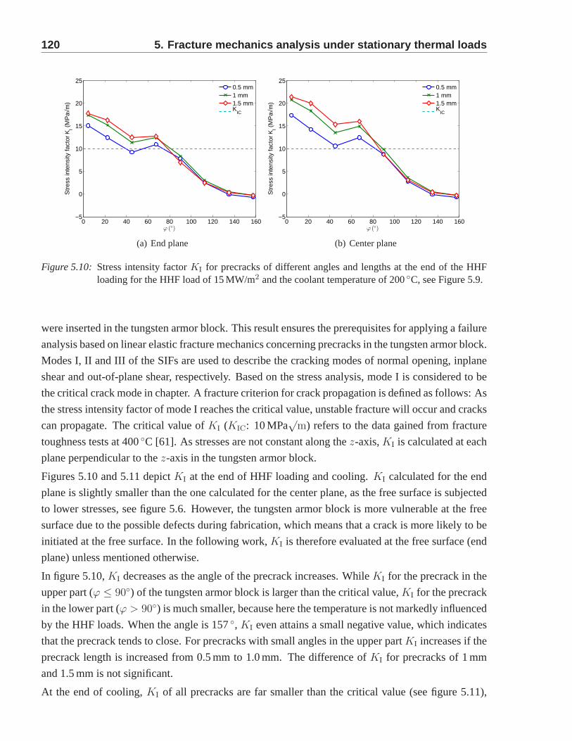
120 5. Fracture mechanics analysis under stationary therma l loads
0 20 40 60 80 100 120 140 160−5
0
5
10
15
20
25
ϕ (◦)
Str
ess
inte
nsity
fact
or K
I (M
Pa√
m)
0.5 mm1 mm1.5 mmK
IC
(a) End plane
0 20 40 60 80 100 120 140 160−5
0
5
10
15
20
25
ϕ (◦)
Str
ess
inte
nsity
fact
or K
I (M
Pa√
m)
0.5 mm1 mm1.5 mmK
IC
(b) Center plane
Figure 5.10: Stress intensity factorKI for precracks of different angles and lengths at the end of the HHFloading for the HHF load of 15 MW/m2 and the coolant temperature of 200◦C, see Figure 5.9.
were inserted in the tungsten armor block. This result ensures the prerequisites for applying a failure
analysis based on linear elastic fracture mechanics concerning precracks in the tungsten armor block.
Modes I, II and III of the SIFs are used to describe the cracking modes of normal opening, inplane
shear and out-of-plane shear, respectively. Based on the stress analysis, mode I is considered to be
the critical crack mode in chapter. A fracture criterion forcrack propagation is defined as follows: As
the stress intensity factor of mode I reaches the critical value, unstable fracture will occur and cracks
can propagate. The critical value ofKI (KIC: 10 MPa√
m) refers to the data gained from fracture
toughness tests at 400◦C [61]. As stresses are not constant along thez-axis,KI is calculated at each
plane perpendicular to thez-axis in the tungsten armor block.
Figures 5.10 and 5.11 depictKI at the end of HHF loading and cooling.KI calculated for the end
plane is slightly smaller than the one calculated for the center plane, as the free surface is subjected
to lower stresses, see figure 5.6. However, the tungsten armor block is more vulnerable at the free
surface due to the possible defects during fabrication, which means that a crack is more likely to be
initiated at the free surface. In the following work,KI is therefore evaluated at the free surface (end
plane) unless mentioned otherwise.
In figure 5.10,KI decreases as the angle of the precrack increases. WhileKI for the precrack in the
upper part (ϕ ≤ 90◦) of the tungsten armor block is larger than the critical value,KI for the precrack
in the lower part (ϕ > 90◦) is much smaller, because here the temperature is not markedly influenced
by the HHF loads. When the angle is 157◦, KI even attains a small negative value, which indicates
that the precrack tends to close. For precracks with small angles in the upper partKI increases if the
precrack length is increased from 0.5 mm to 1.0 mm. The difference ofKI for precracks of 1 mm
and 1.5 mm is not significant.
At the end of cooling,KI of all precracks are far smaller than the critical value (seefigure 5.11),
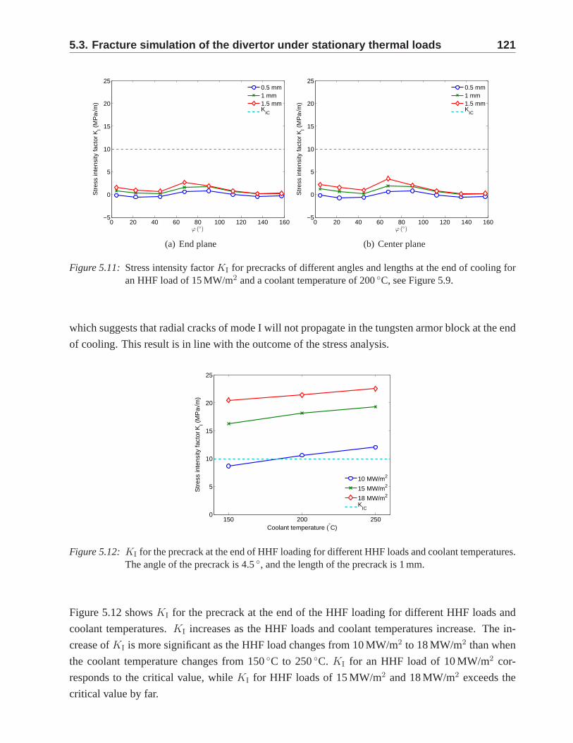
5.3. Fracture simulation of the divertor under stationary t hermal loads 121
0 20 40 60 80 100 120 140 160−5
0
5
10
15
20
25
ϕ (◦)
Str
ess
inte
nsity
fact
or K
I (M
Pa√
m)
0.5 mm1 mm1.5 mmK
IC
(a) End plane
0 20 40 60 80 100 120 140 160−5
0
5
10
15
20
25
ϕ (◦)
Str
ess
inte
nsity
fact
or K
I (M
Pa√
m)
0.5 mm1 mm1.5 mmK
IC
(b) Center plane
Figure 5.11: Stress intensity factorKI for precracks of different angles and lengths at the end of cooling foran HHF load of 15 MW/m2 and a coolant temperature of 200◦C, see Figure 5.9.
which suggests that radial cracks of mode I will not propagate in the tungsten armor block at the end
of cooling. This result is in line with the outcome of the stress analysis.
150 200 2500
5
10
15
20
25
Coolant temperature (°C)
Str
ess
inte
nsity
fact
or K
I (M
Pa√
m)
10 MW/m2
15 MW/m2
18 MW/m2
KIC
Figure 5.12: KI for the precrack at the end of HHF loading for different HHF loads andcoolant temperatures.The angle of the precrack is 4.5◦, and the length of the precrack is 1 mm.
Figure 5.12 showsKI for the precrack at the end of the HHF loading for different HHF loads and
coolant temperatures.KI increases as the HHF loads and coolant temperatures increase. The in-
crease ofKI is more significant as the HHF load changes from 10 MW/m2 to 18 MW/m2 than when
the coolant temperature changes from 150◦C to 250◦C. KI for an HHF load of 10 MW/m2 cor-
responds to the critical value, whileKI for HHF loads of 15 MW/m2 and 18 MW/m2 exceeds the
critical value by far.
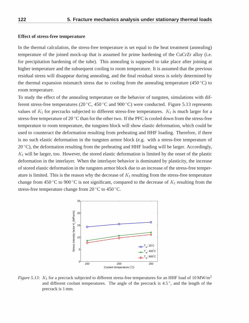
122 5. Fracture mechanics analysis under stationary therma l loads
Effect of stress-free temperature
In the thermal calculation, the stress-free temperature isset equal to the heat treatment (annealing)
temperature of the joined mock-up that is assumed for prime hardening of the CuCrZr alloy (i.e.
for precipitation hardening of the tube). This annealing issupposed to take place after joining at
higher temperature and the subsequent cooling to room temperature. It is assumed that the previous
residual stress will disappear during annealing, and the final residual stress is solely determined by
the thermal expansion mismatch stress due to cooling from the annealing temperature (450◦C) to
room temperature.
To study the effect of the annealing temperature on the behavior of tungsten, simulations with dif-
ferent stress-free temperatures (20◦C, 450◦C and 900◦C) were conducted. Figure 5.13 represents
values ofKI for precracks subjected to different stress-free temperatures. KI is much larger for a
stress-free temperature of 20◦C than for the other two. If the PFC is cooled down from the stress-free
temperature to room temperature, the tungsten block will show elastic deformation, which could be
used to counteract the deformation resulting from preheating and HHF loading. Therefore, if there
is no such elastic deformation in the tungsten armor block (e.g. with a stress-free temperature of
20◦C), the deformation resulting from the preheating and HHF loading will be larger. Accordingly,
KI will be larger, too. However, the stored elastic deformation is limited by the onset of the plastic
deformation in the interlayer. When the interlayer behavioris dominated by plasticity, the increase
of stored elastic deformation in the tungsten armor block due to an increase of the stress-free temper-
ature is limited. This is the reason why the decrease ofKI resulting from the stress-free temperature
change from 450◦C to 900◦C is not significant, compared to the decrease ofKI resulting from the
stress-free temperature change from 20◦C to 450◦C.
150 200 2500
5
10
15
20
25
Coolant temperature (°C)
Str
ess
inte
nsity
fact
or K
I (M
Pa√
m)
Tsf
: 20°C
Tsf
: 450°C
Tsf
: 900°C
Figure 5.13: KI for a precrack subjected to different stress-free temperatures for an HHF load of 10 MW/m2
and different coolant temperatures. The angle of the precrack is 4.5◦, and the length of theprecrack is 1 mm.
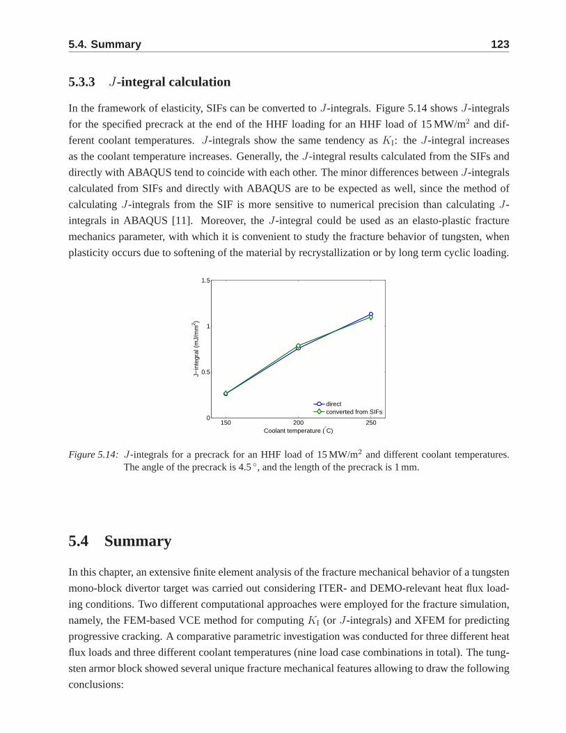
5.4. Summary 123
5.3.3 J-integral calculation
In the framework of elasticity, SIFs can be converted toJ-integrals. Figure 5.14 showsJ-integrals
for the specified precrack at the end of the HHF loading for an HHF load of 15 MW/m2 and dif-
ferent coolant temperatures.J-integrals show the same tendency asKI: the J-integral increases
as the coolant temperature increases. Generally, theJ-integral results calculated from the SIFs and
directly with ABAQUS tend to coincide with each other. The minor differences betweenJ-integrals
calculated from SIFs and directly with ABAQUS are to be expected as well, since the method of
calculatingJ-integrals from the SIF is more sensitive to numerical precision than calculatingJ-
integrals in ABAQUS [11]. Moreover, theJ-integral could be used as an elasto-plastic fracture
mechanics parameter, with which it is convenient to study the fracture behavior of tungsten, when
plasticity occurs due to softening of the material by recrystallization or by long term cyclic loading.
150 200 2500
0.5
1
1.5
Coolant temperature (°C)
J−in
tegr
al (
mJ/
mm
2 )
directconverted from SIFs
Figure 5.14: J-integrals for a precrack for an HHF load of 15 MW/m2 and different coolant temperatures.The angle of the precrack is 4.5◦, and the length of the precrack is 1 mm.
5.4 Summary
In this chapter, an extensive finite element analysis of the fracture mechanical behavior of a tungsten
mono-block divertor target was carried out considering ITER- and DEMO-relevant heat flux load-
ing conditions. Two different computational approaches were employed for the fracture simulation,
namely, the FEM-based VCE method for computingKI (or J-integrals) and XFEM for predicting
progressive cracking. A comparative parametric investigation was conducted for three different heat
flux loads and three different coolant temperatures (nine load case combinations in total). The tung-
sten armor block showed several unique fracture mechanicalfeatures allowing to draw the following
conclusions:
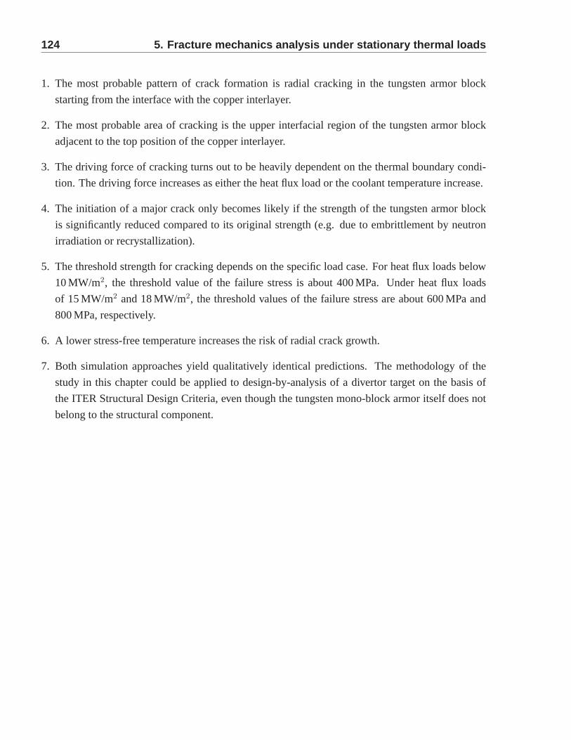
124 5. Fracture mechanics analysis under stationary therma l loads
1. The most probable pattern of crack formation is radial cracking in the tungsten armor block
starting from the interface with the copper interlayer.
2. The most probable area of cracking is the upper interfacial region of the tungsten armor block
adjacent to the top position of the copper interlayer.
3. The driving force of cracking turns out to be heavily dependent on the thermal boundary condi-
tion. The driving force increases as either the heat flux loador the coolant temperature increase.
4. The initiation of a major crack only becomes likely if the strength of the tungsten armor block
is significantly reduced compared to its original strength (e.g. due to embrittlement by neutron
irradiation or recrystallization).
5. The threshold strength for cracking depends on the specific load case. For heat flux loads below
10 MW/m2, the threshold value of the failure stress is about 400 MPa. Under heat flux loads
of 15 MW/m2 and 18 MW/m2, the threshold values of the failure stress are about 600 MPaand
800 MPa, respectively.
6. A lower stress-free temperature increases the risk of radial crack growth.
7. Both simulation approaches yield qualitatively identical predictions. The methodology of the
study in this chapter could be applied to design-by-analysis of a divertor target on the basis of
the ITER Structural Design Criteria, even though the tungsten mono-block armor itself does not
belong to the structural component.
125
Chapter 6
General conclusions and outlook
6.1 General conclusions
Nearly all plasma-facing surfaces in the International Thermonuclear Experimental Reactor (ITER)
are/will be armored with tungsten. Also, tungsten is the most promising armor material for the
plasma-facing components of the DEMOnstration power plant(DEMO). However, the inherent brit-
tleness of tungsten at low temperature is a very critical issue to the reliability of the plasma-facing
components. The aim of this dissertation is to understand and predict the brittle failure of tungsten
under high heat flux loads using numerical approaches.
In this dissertation, three relevant high heat flux loads areconsidered: short transient thermal loads
by edge localized mode (ELM), slow high-energy-depositionthermal loads (e.g. vertical displace-
ment events (VDEs)) and stationary heat flux loads. Two-dimensional numerical simulations were
performed for short transient thermal loads and slow high-energy-deposition thermal loads accord-
ing to the corresponding electron beam irradiation tests. Athree-dimensional finite element model
was built to be able to study the failure behavior of the tungsten armored divertor under stationary
heat flux loads.
The tungsten armor’s thermal and mechanical responses to the three loading events were analyzed
in detail. The maximum temperature under ELM-like transient thermal loads is in general below
the melting point of tungsten for the power densities of 0.3-1.3 GW/m2 at base temperatures of 20-
800◦C. For slow high-energy-deposition thermal loads, the maximum temperature is usually above
the melting point of tungsten due to its long loading pulse. However, if the loading is constrained
to a small area, the temperature can be kept below the meltingpoint of tungsten. The maximum
temperatures in the armored tungsten divertor under ITER and DEMO relevant stationary heat flux
(10-18 MW/m2) with a coolant temperature up to 250◦C are below 1600◦C.
Plastic strains are generated at the surface of tungsten armors under ELM-like transient thermal loads
and slow high-energy-deposition thermal loads, while there is almost no plastic strain in the tungsten
armor block of the divertor under purely stationary loading. Tensile residual stress is generated
126 6. General conclusions and outlook
during cooling for the ELM-like transient thermal loads andslow high-energy-deposition thermal
loads. This residual stress turns out to be critical for cracking at the surface of the tungsten armor.
For the stationary heat flux loads, the level of stress is muchlower than that for transient thermal
loads. In contrast to the transient thermal cases where the residual stress during cooling plays an
important role, thermal stress during heating is the most critical stress for cracking in the tungsten
block of the divertor under stationary heat flux loads. In thetungsten divertor, stress concentration
occurs in the upper part of the tungsten block and close to theinterlayer. The temperature in this area
is below or close to the ductile-to-brittle transition temperature (DBTT) during the stationary heat
flux loading, which increases the risk of a brittle failure oftungsten material. In general, cracking of
tungsten is likely to occur during cooling for the transientthermal loads and during heating for the
stationary heat flux loads.
Based on the different features of the three loading scenarios, fracture mechanical investigations
were carried out with the help of the weight function method,the extended finite element method
(XFEM) and the FEM-based virtual crack extension (VCE) method. Several conclusions are drawn
from the fracture mechanics study for the three loading scenarios:
Short transient thermal loads
1. When the loading area is sufficiently large, the simplified analytical solution based on a semi-
infinite space assumption can give good estimates of temperature, stress and strain in the central
part of the loading area.
2. Cracking of tungsten under ELM-like transient thermal loads is due to the residual stress that
is generated during cooling. Cracking occurs at the surface when the ductility of tungsten is
significantly reduced as the temperature drops below DBTT.
3. The failure map, which is created by comparing theJ-integrals for precracks with the critical
energy release rate obtained from the fracture toughness tests, shows a reasonable agreement
with the experimentally observed results. The crack formation is predicted for the power density
of 0.6 GW/m2 and above, and when the base temperature is higher than 600◦C, almost no cracks
is predicted. An efficient way to prevent brittle cracking oftungsten is to operate the tungsten
armor at the temperatures above the threshold temperature.
4. A ramp pulse with a longer duration leads to lower temperatures and stresses in comparison to a
constant pulse with a shorter duration. Yet, the differenceis moderate when both their maximum
power density and total deposited energy are identical.
5. Compared to the triangular loading, cracks produced at theedge of the loading area under the
uniform loading are more likely to grow further in parallel to the loading surface.
6.2. Outlook 127
Slow high-energy-deposition thermal loads
1. When the loading area of the slow high-energy-deposition thermal loads is limited, the maximum
temperature can be kept below the melting point of tungsten.A nearly steady-state of the tem-
perature profile at the surface of tungsten can be reached after several milliseconds of the slow
high-energy-deposition thermal loading.
2. In the experiments, recrystallization of tungsten couldbe observed after slow high-energy-deposition
thermal loads in case the numerical prediction of the maximum temperature, which coincides with
the temperature measurements, was above the recrystallization temperature of tungsten, even with
a loading duration of only 0.5 s.
3. The good agreement between the experimental observations and the numerical predictions proves
the validity of the computational approaches. The method used in this dissertation can therefore
serve as an adequate basis for the design of divertors in fusion reactors.
Stationary heat flux loads
1. Stationary heat flux loads do not cause severe plastic deformation in the tungsten armor block of
the divertor. The cracking due to stationary heat flux loads occurs most likely near the coolant
pipe in the tungsten armor block due to the tensile thermal stress. The most probable pattern of
crack formation is radial cracking in the tungsten armor block starting at the interface with the
copper interlayer.
2. Under stationary heat flux loads, stress is not critical inthe tungsten armor block as long as no
severe material degradation occurs.
3. The joining technique of the divertor has significant impact on the stress distribution in the tung-
sten armor block (e.g. a lower stress-free temperature increases the risk of radial crack growth.).
6.2 Outlook
In this dissertation, the numerical predictions generallycoincide with the experimental observations.
However, there is still much space to improve the accuracy ofthe current numerical results. A
promising approach would be to compile a more detailed material characterization, as follows:
(1) Thermal and mechanical properties of tungsten should beinvestigated under cyclic thermal load-
ings and in operationally relevant environments. The high fluxes of energetic neutrons, hydrogen
and helium ions, as well as a bombardment by helium isotopes may degrade the thermal and me-
chanical properties of tungsten.

128 6. General conclusions and outlook
(2) As the plasma-facing components will be exposed to stationary heat flux for longer time periods
while in operation, creep can occur due to the critical exposure time and exposure temperature.
Considering the corresponding material parameter in the calculation may help to obtain more
realistic results.
(3) Microstructure characterizations (e.g. grain size, material properties at grain boundaries, grain
orientations and pore distributions) of tungsten or tungsten alloys should be determined in de-
tail, as microstructure features have significant impact onthe behavior of a material. Once a
micromechanical finite element model is established, a multiscale model can serve to transfer
the results obtained at the microscopic to the macroscopic scale.
From the result of this study, it becomes evident that cracking of tungsten is inevitable under some
ITER relevant transient thermal loadings. Therefore, future work should address numerical investi-
gations concerning the development of cracks based on a moredetailed model (e.g. a microstructure
model). Once the cracking patterns are understood and can becontrolled, strategies can be developed
to conquer the material weakness. One possibility is to use atungsten composite instead of tungsten
and tungsten alloys. The composite concept cannot only improve the material properties (e.g. the
reinforcement with tungsten fibers, which is considered as away to retain tungsten toughness even
under conditions of embrittlement), but also help to control the cracking patterns. Furthermore, mod-
elling of thermal fatigue of tungsten under ITER relevant thermal loadings will be of great interest to
the component design in case that the proper material data can be obtained from the corresponding
tests.
Appendix A. Frederick-Armstrong model 129
Appendix A
Frederick-Armstrong model
Considering asymmetric hardening, the von Mises yield criterion is given by
Fpotential = [3
2(S− ααα′) : (S− ααα′)]0.5 − σeε
pe = 0, (A.1)
whereFpotential is the plastic potential in the sense of the associated flow rule, S the deviatoric stress
tensor,ααα′ the deviatoric backstress tensor,σe the equivalent stress andεpe the equivalent plastic strain.
The backstress tensorα stands for the yield surface displacement in a stress space,whereasσe
indicates the size of the yield surface. The non-linear kinematic hardening law is expressed as [83]
ααα =C
σe
(σσσ − ααα)εpe − γαααεp
e, (A.2)
whereααα is the backstress rate tensor,C is the initial kinematic hardening modulus,σσσ is the stress
tensor,εpe is the equivalent plastic strain rate andγ is a constant determining the rate at which
the kinematic hardening modulus decreases with increasingplastic strain. C and γ are material
parameters to be calibrated. The first term in A.2 is the contribution of Ziegler’s linear kinematic
hardening, and the second one is the non-linear relaxation term. The non-linear isotropic hardening
law is expressed as
σe = σ0 + Q[1 − exp(−bεpe)], (A.3)
whereσ0 is the initial size of the yield surface,Q the maximum change in the size of the yield surface
andb defines the rate at which the size of the yield surface changesas plastic straining progresses.
Q and b are material parameters to be calibrated. The five material parameters of the combined
nonlinear hardening law are calibrated by fitting method using the stabilized loops of unidirectional

130 A. Frederick-Armstrong model
strain controlled cyclic tension-compression tests [78].
131
Bibliography
[1] BP p.l.c, BP Energy Outlook 2030, London, United Kingdom, 2013.
[2] European Fusion Development Agreement, Tokamaks, 2014, http://www.efda.org/fusion/fusion-machine/types-of-fusion-machines/tokamaks.
[3] M. Merola, D. Loesser, A. Martin, P. Chappuis, R. Mitteaua,V. Komarova, R. Pitts, S. Gic-quel, V. Barabash, L. Giancarli, J. Palmer, M. Nakahira, A. Loarte, D. Campbell, R. Eaton,A. Kukushkin, M. Sugihara, F. Zhang, C. Kim, R. Raffray, L. Ferrand, D. Yao, S. Sadakov,A. Furmanek, V. Rozov, T. Hirai, F. Escourbiac, T. Jokinen, B. Calcagno, S. Mori, ITERplasma-facing components, Fusion Engineering and Design 85 (2010) 2312–2322.
[4] T. Hirai, K. Ezato, P. Majerus, ITER relevant high heat flux testing on plasma facing surfaces,Materials Transactions, The Japan Institute of Metals 46 (2005) 412–424.
[5] M. Rodig, M. Akiba, P. Chappuis, R. Duwe, M. Febvre, A. Gervash, J. Linke, N. Litounovsky,S. Suzuki, B. Wiechers, D. Youchison, Comparison of electron beam test facilities for testingof high heat flux components, Fusion Engineering and Design 51-52 (2000) 715–722.
[6] E. Visca, B. Riccardi, A. Orsini, C. Testani, Manufacturingand testing of monoblock tungstensmall-scale mock-ups, Fusion Engineering and Design 56-57(2001) 343–347.
[7] Siemens AG, Internal report on physical parameters of tungsten, 1995.
[8] PLANSEE, Tungsten material properties and applications, 2014,http://www.plansee.com/en/Materials-Tungsten-403.htm.
[9] J.-H. You, M. Miskiewicz, Material parameters of copperand CuCrZr alloy for cyclic plasticityat elevated temperatures, Journal of Nuclear Materials 373(2008) 269–274.
[10] ITER Structural Design Criteria for In-vessel Components (SDC-IC), ITER Document No. G74 MA 8 01-05-28 W0.2, 2008.
[11] Abaqus analysis user’s manual 6.12., Dassault Systemes Simulia Corp., Providence, RI, USA,2012.
[12] Wikipedia, Nuclear binding energy, 2014,http://en.wikipedia.org/wiki/Nuclear_binding_energy.
[13] S. Glasstone, R. H. Lovberg, Controlled thermonuclear reactions, 1960.
132 Bibliography
[14] C. M. Braams, P. E. Stott, Nuclear Fusion: Half a Century of Magnetic Confinement FusionResearch, Taylor & Francis, 2002.
[15] ITER, The ITER story, 2014,http://www.iter.org/proj/iterhistory.
[16] V. Barabash, M. Akiba, I. Mazul, M. Ulrickson, G. Vieider, Selection, development and char-acterisation of plasma facing materials for ITER, Journal ofNuclear Materials 233-237 (1996)718–723.
[17] T. Hirai, H. Maier, M. Rubel, P. Mertens, R. Neu, E. Gauthier, J. Likonen, C. Lungu, G. Mad-daluno, G. Matthews, R. Mitteau, O. Neubauer, G. Piazza, V.Philipps, B. Riccardi, C. Ruset,I. Uytdenhouwen, R& D on full tungsten divertor and berylliumwall for JET ITER-like wallproject, Fusion Engineering and Design 82 (2007) 1839 – 1845.
[18] F. Elio, K. Ioki, P. Barabaschi, L. Bruno, A. Cardella, M. Hechler, T. Kodama, A. Lodato,D. Loesser, D. Lousteau, N. Miki, K. Mohri, R. Parker, R. Raffray, D. Williamson, M. Yamada,W. Daenner, R. Mattas, Y. Strebkov, H. Takatsu, Engineering design of the ITER blanket andrelevant research and development results, Fusion Engineering and Design 46 (1999) 159–175.
[19] D. Rupp, S. M. Weygand, Loading rate dependence of the fracture toughness of polycrystallinetungsten, Journal of Nuclear Materials 417 (2011) 477–480.
[20] A. A. Griffith, The phenomena of rupture and flow in solids, Philosophical Transactions of theRoyal Society of London 221 (1921) 163–198.
[21] G. Irwin, Analysis of stresses and strains near the end of a crack traversing a plate, Journal ofApplied Mechanics 24 (1957) 361–364.
[22] H. Tada, P. C. Paris, G. R. Irwin, The Stress Analysis of Cracks Handbook, 3rd Edition, Amer-ican Society of Mechanical Engineers Press, 2001.
[23] D. P. Rooke, D. J. Cartwright, Compendium of Stress Intensity Factors, Her Majesty’s Sta-tionery Office, 1976.
[24] J. R. Rice, A path independent integral and approximate analysis of strain concentration bynotches and cracks, Journal of Applied Mechanics 35 (1968) 379–386.
[25] H. Buckner, A novel principle for the computation of stress intensity factors, Journal of AppliedMathematics and Mechanics 50 (1970) 529–546.
[26] T. Fett, D. Munz, Stress intensity factors and weight functions, Computational Mechanics Pub-lications, Southampton, 1997.
[27] G. Glinka, G. Shen, Universal features of weight functions for cracks in mode I, EngineeringFracture Mechanics 40 (1991) 1135–1146.
[28] C. F. Shih, B. Moran, T. Nakamura, Energy release rate along a three-dimensional crack frontin a thermally stressed body, International Journal of Fracture 30 (1986) 79–102.
[29] Y. Lei, N. P. O’Dowd, G. A. Webester, Fracture mechanicsanalysis of a crack in a residualstress field, International Journal of Fracture 106 (2000) 195–216.
Bibliography 133
[30] J. F. Yau, S. S. Wang, H. T. Corten, A mixed-mode crack analysis of isotropic solids usingconservation laws of elasticity, Journal of Applied Mechanics 47 (1980) 335–341.
[31] T. Belytschko, T. Black, Elastic crack growth in finite elements with minimal remeshing, Inter-national Journal for Numerical Methods in Engineering 45 (1999) 601–620.
[32] J. M. Melenk, I. Babuska, The partition of unity finite element method: Basic theory andapplications, Computer Methods in Applied Mechanics and Engineering 139 (1996) 289–314.
[33] S. Osher, J. A. Sethian, Fronts propagating with curvature dependent speed: Algorithms basedon Hamilton-Jacobi formulations, Journal of ComputationalPhysics 79 (1988) 12–49.
[34] M. Stolarska, D. Chopp, N. Moes, T. Belytschko, Modelling crack growth by level sets in theextended finite element method, International Journal for Numerical Methods in Engineering51 (2001) 943–960.
[35] N. Moes, J. Dolbow, T. Belytscheko, A finite element method for crack growth without remesh-ing, International Journal for Numerical Methods in Engineering 46 (1999) 131–150.
[36] F. Wagner, G. Becker, K. Behringer, D. Campbell, A. Eberhagen, W. Engelhardt, G. Fussmann,O. Gehre, J. Gernhardt, G. v. Gierke, G. Haas, M. Huang, F. Karger, M. Keilhacker, O. Kluber,M. Kornherr, K. Lackner, G. Lisitano, G. G. Lister, H. M. Mayer, D. Meisel, E. R. Muller,H. Murmann, H. Niedermeyer, W. Poschenrieder, H. Rapp, H. Rohr, F. Schneider, G. Siller,E. Speth, A. Stabler, K. H. Steuer, G. Venus, O. Vollmer, Z. Yu, Regime of improved con-finement and high beta in neutral-beam-heated divertor discharges of the ASDEX tokamak,Physical Review Letters 49 (1982) 1408.
[37] H. Zohm, Edge localized modes (ELMs), Plasma Physics and Controlled Fusion 38 (1996)105.
[38] P. Monier-Garbet, P. Andrew, P. Belo, G. Bonheure, Y. Corre, K. Crombe, P. Dumortier, T. Eich,R. Felton, J. Harling, J. Hogan, A. Huber, S. Jachmich, E. Joffrin, H. Koslowski, A. Kreter,G. Maddison, G. Matthews, A. Messiaen, M. Nave, J. Ongena, V.Parail, M. Puiatti, J. Rapp,R. Sartori, J. Stober, M. Tokar, B. Unterberg, M. Valisa, I. Voitsekhovitch, M. von Hellermann,JET-EFDA contributors, Impurity-seeded ELMy H-modes in JET, with high density and re-duced heat load, Nuclear Fusion 45 (2005) 1404–1410.
[39] A. W. Degeling, Y. R. Martin, J. B. Lister, L. Villard, V. N.Dokouka, V. E. Lukash, R. R.Khayrutdinov, Magnetic triggering of ELMs in TCV, Plasma Physics and Controlled Fusion45 (2003) 1637.
[40] P. Lang, G. Conway, T. Eich, L. Fattorini, O. Gruber, S. Gunter, L. Horton, S. Kalvin,A. Kallenbach, M. Kaufmann, G. Kocsis, A. Lorenz, M. Manso, M. Maraschek, V. Mertens,J. Neuhauser, I. Nunes, W. Schneider, W. Suttrop, H. Urano, the ASDEX Upgrade Team, ELMpace making and mitigation by pellet injection in ASDEX upgrade, Nuclear Fusion 44 (2004)665.
[41] T. E. Evans, R. A. Moyer, K. H. Burrell, M. E. Fenstermacher, I. Joseph, A. W. Leonard,T. H. Osborne, G. D. Porter, M. J. Schaffer, P. B. Snyder, P. R. Thomas, J. G. Watkins, W. P.
134 Bibliography
West, Edge stability and transport control with resonant magnetic perturbations in collisionlesstokamak plasmas, Nature Physics 2 (2006) 419–423.
[42] B. Hudson, T. Evans, T. Osborne, C. Petty, P. Snyder, E. Unterberg, ELM suppression byresonant magnetic perturbation in high-performance, stationary plasmas, Nuclear Fusion 50(2010) 045006.
[43] A. Loarte, M. Sugihara, M. Shimada, A. Kukushkin, D. Campbell, M. Pick, C. Lowry,M. Merola, R. Pitts, V. Riccardo, G. Arnoux, W. Fundamenski, G.Matthews, S. Pinches,A. Kirk, E. Nardon, T. Eich, A. Herrmann, G. Pautasso, A. Kallenbach, Power and particlefluxes at the plasma edge of ITER: Specifications and physics basis, 22nd IAEA Fusion En-ergy Conference, Geneva, Switzerland, 2008.
[44] N. Klimov, V. Podkovyrov, A. Zhitlukhin, D. Kovalenko,B. Bazylev, G. Janeschitz, I. Land-man, S. Pestchanyi, G. Federici, A. Loarte, M. Merola, J. Linke, T. Hirai, J. Compan, Anexperimental study of PFCs erosion under ITER-like transientloads at plasma gun facilityQSPA, 18th PSI Conference, Toledo, Spain, 2008.
[45] G. Federici, A. Loarte, G. Strohmayer, Assessment of erosion of the ITER divertor targetsduring type I ELMs, Plasma Physics and Controlled Fusion 45 (2003) 1523.
[46] T. Hirai, G. Pintsuk, J. Linke, M. Batilliot, Cracking failure study of ITER-reference tungstengrade under single pulse thermal shock loads at elevated temperatures, Journal of NuclearMaterials 390-391 (2009) 751–754.
[47] G. Pintsuk, A. Prokhodtseva, I. Uytdenhouwen, Thermalshock characterization of tungstendeformed in two orthogonal directions, Journal of Nuclear Materials 417 (2011) 481–486.
[48] M. Wirtz, J. Linke, G. Pintsuk, L. Singheiser, I. Uytdenhouwen, Comparison of the thermalshock performance of different tungsten grades and the influence of microstructure on the dam-age behaviour, Physica Scripta T145 (2011) 014058.
[49] J. Linke, T. Loewenhoff, V. Massaut, G. Pintsuk, G. Ritz,M. Roedig, A. Schmidt, C. Thomser,I. Uytdenhouwen, V. Vasechko, M. Wirtz, Performance of different tungsten grades under tran-sient thermal loads, Nuclear Fusion 51 (2011) 073017.
[50] I. Garkusha, I. Landman, J. Linke, V. Makhlaj, A. Medvedev, S. Malykhin, S. Peschanyi,G. Pintsuk, A. Pugachev, V. Tereshin, Performance of deformed tungsten under ELM-likeplasma exposures in QSPA Kh-50, Journal of Nuclear Materials 415 (2011) 481–486.
[51] S. E. Pestchanyi, J. Linke, Simulation of cracks in tungsten under ITER specific transient heatloads, Fusion Engineering and Design 82 (2007) 1657–1663.
[52] T. Hirai, G. Pintsuk, Thermo-mechanical calculationson operation temperature limits of tung-sten as plasma facing material, Fusion Engineering and Design 82 (2007) 389–393.
[53] K. Kamiya, N. Asakura, J. Boedo, T. Eich, G. Federici, M. Fenstermacher, K. Finken, A. Her-rmann, J. Terry, A. kirk, B. Koch, A. Loarte, R. Maingi, R. Maqueda, E. Nardon, N. Oyama,R. Sartori, Edge localized modes: Recent experimental findings and related issues, PlasmaPhysics and Controlled Fusion 49 (2007) S43.
Bibliography 135
[54] J. Linke, H. Bolt, R. Duwe, W. Kuhnlein, A. Lodato, M. Rodig, K. Schopflin, B. Wiechers,High heat flux simulation experiments with improved electron beam diagnostics, Journal ofNuclear Materials 283-287 (2000) 1152–1156.
[55] I. Uytdenhouwen, M. Decreton, T. Hirai, J. Linke, G. Pintsuk, G. V. Oost, Influence of recrys-tallization on thermal shock resistance of various tungsten grades, Journal of Nuclear Materials363-365 (2007) 1099–1103.
[56] G. Pintsuk, Armour material optimisation-testing of tungsten under high cyclic transient ther-mal loads, Presented at the EFDA-Meeting, Garching, Germany, 2011.
[57] A. Faghri, Y. Zhang, Transport Phenomena in MultiphaseSystems, Elsevier, 2006.
[58] H. S. Carslaw, J. C. Jaeger, Conduction of Heat in Solids, 2nd Edition, Oxford University Press,New York, 1959.
[59] W. Mack, U. Gamer, Stress distribution in an elastic plastic disk subjected to a circular heatsource, Journal of Thermal Stresses 6 (1983) 323–336.
[60] M. Ishihara, Y. Tanigawa, R. Kawamura, N. Noda, Theoretical analysis of thermoelastoplasticdeformation of a circular plate due to a partially distributed heat supply, Journal of ThermalStresses 20 (1997) 203–225.
[61] B. Gludovatz, S. Wurster, A. Hoffmann, R. Pippan, Fracture toughness of polycrystalline tung-sten alloys, International Journal of Refractory Metals andHard Materials 28 (2010) 674–678.
[62] I. Uytdenhouwen, Degradation of first wall materials under ITER relevant loading conditions,Ph.D. thesis, University Gent (2011).
[63] G. D. Temmerman, J. Zielinski, S. van Diepen, L. Marot, M. Price, ELM simulation exper-iments on Pilot-PSI using simultaneous high flux plasma and transient heat/particle source,Nuclear Fusion 51 (2011) 073008.
[64] P. Gumbsch, Brittle fracture and the brittle-to-ductile transition of tungsten, Journal of NuclearMaterials 323 (2003) 304–312.
[65] B. Riccardi, P. Gavila, R. Giniatulin, V. Kuznetsov, R. Rulev, N. Klimov, D. Kovalenko, V. Bar-suk, V. Koidan, S. Korshunov, Effect of stationary high heatflux and transient ELMs-like heatloads on the divertor PFCs, Fusion Engineering and Design 88 (2013) 1673 – 1676.
[66] A. Huber, A. Arakcheev, G. Sergienko, I. Steudel, M. Wirtz, A. V. Burdakov, J. W. Coenen,A. Kreter, J. Linke, P. Mertens, V. Philipps, G. Pintsuk, M. Reinhart, U. Samm, A. Shoshin,B. Schweer, B. Unterberg, M. Zlobinski, Investigation of the impact of transient heat loadsapplied by laser irradiation on ITER-grade tungsten, Physica Scripta T159 (2014) 014005.
[67] T. Dummr, J. C. Lasalvia, G. Ravichandran, M. A. Meyers, Effect of strain rate on plastic flowand failure in polycrystalline tungsten, Acta Metallurgica 46 (1998) 6267–6290.
[68] G. Ambrosino, M. Ariola, G. D. Tommasi, A. Pironti, Plasma vertical stabilization in the ITERtokamak via constrained static output feedback, Transactions on Control Systems Technology19 (2011) 376–381.
136 Bibliography
[69] J. M. Linke, T. Hirai, M. Rodig, L. A. Singheiser, Performance of plasma-facing materialsunder intense thermal loads in tokamaks and stellarators, Fusion Science and Technology 46(2004) 142–151.
[70] A. Cardella, H. Gorenflo, A. Lodato, K. Ioki, R. Raffray, Effects of plasma disruption eventson ITER first wall materials, Journal of Nuclear Materials 283-287 (2000) 1105–1110.
[71] J. Linke, P. Lorenzetto, P. Majerus, M. Merola, D. Pitzer, M. Roedig, EU development of highheat flux components, Fusion Science and Technology 47 (2005) 678–685.
[72] M. Sommerer, Multiple-Use-Technologie der Fusionsforschung: Mikrostrukturelle Aspektedes thermozyklischen Bruchverhaltens von Wolfram in industrieller Anwendung, Ph.D. thesis,Technische Universitat Munchen (in preparation).
[73] J. Linke, High heat flux performance of plasma facing materials and components under serviceconditions in future fusion reactors, Fusion Science and Technology 49 (2006) 455–464.
[74] Y. Ishijima, H. Kurishita, K. Yubuta, H. Arakawa, M. Hasegawa, Y.Hiraoka, T. Takida,K. Takebe, Current status of ductile tungsten alloy development by mechanical alloying, Jour-nal of Nuclear Materials 775 (2004) 329–333.
[75] J.-H. You, I. Komarova, Probabilistic failure analysis of a water-cooled tungsten divertor: Im-pact of embrittlement, Journal of Nuclear Materials 375 (2008) 283–289.
[76] M. Miskiewicz, J.-H. You, Impact of plastic softening of over-aged CuCrZr alloy heat sink tubeon the structural reliability of a plasma-facing component, Fusion Engineering and Design 83(2008) 66–71.
[77] J. P. Blanchard, C. Martin, Fracture and creep in an all-tungsten divertor for ARIES, FusionScience and Technology 64 (2013) 435–439.
[78] D. Maisonnier, I. Cook, P. Sardain, R. Andreani, L. D. Pace, R. Forrest, L. Giancarli,S. Hermsmeyer, P. Norajitra, N. Taylor, A conceptual study of commercial fusion power plants,EFDA(05)-27/4.10, 2005.
[79] F. Crescenzi, A. Moriani, S. Roccella, E. Visca, M. Richou,Water-cooled divertor target designstudy CuCrZr/W monoblock concept, EFDA report: TA WP13-DAS02-T02-D02, 2013.
[80] J. Lemaitre, J.-L. Chaboche, Mechanics of Solid Materials, 1st Edition, Cambridge UniversityPress, 1994.
[81] P. J. Armstrong, C. O. Frederick, A mathematical representation of the multiaxial Bauschingereffect, G.E.G.B. Report RD/B/N (1966) 731.
[82] J. Chaboche, Constitutive equations for cyclic plasticity and cyclic viscoplasticity, InternationalJournal of Plasticity 5 (1989) 247–302.
[83] M. Lipa, A. Durocher, R. Tivey, T. Huber, B. Schedler, J. Weigert, The use of copper alloyCuCrZr as a structural material for actively cooled plasma facing and in vessel components,Fusion Engineering and Design 75-79 (2005) 469–473.