a numerical study of midaco on 100 minlp...

A Numerical Study of MIDACO on 100 MINLP Benchmarks

Martin Schluter∗, Matthias Gerdts†, Jan-J. Ruckmann∗

∗Theoretical & Computational Optimization Group, University of Birmingham

Birmingham B15 2TT, United Kingdom

[email protected], [email protected]

†Institut fuer Mathematik und Rechneranwendung, Universitaet der Bundeswehr Muenchen,

D-85577 Neubiberg/Muenchen, Germany

[email protected]

January 31, 2012

Abstract

This paper presents a numerical study on MIDACO, a new global optimization softwarefor mixed integer nonlinear programming (MINLP) based on ant colony optimization and theoracle penalty method. Extensive and rigorous numerical tests on a set of 100 non-convexMINLP benchmark problems from the open literature are performed. Results obtained byMIDACO are directly compared to results by a recent study of state of the art deterministicMINLP software on the same test set. Further comparisons with established MINLP soft-ware is undertaken in addition. This study shows, that MIDACO is not only competitiveto established MINLP software, but can even outperform those in terms of number of globaloptimal solutions found. Moreover, the parallelization capabilities of MIDACO enable it to beeven competitive to deterministic software regarding the amount of (serial processed) functionevaluation, while the black-box capabilities of MIDACO offer an intriguing new robustness forMINLP.

Keywords: Mixed Integer Nonlinear Programming (MINLP), Ant Colony Opti-mization, Oracle Penalty Method, Parallel Computing, MIDACO, MISQP, BON-MIN, COUENNE.

1 Introduction

Mixed integer nonlinear programming (MINLP) problems are an important class of optimizationproblems with many real world applications. A mathematical formulation of a MINLP is given in(1), where f(x, y) denotes the objective function to be minimized. In (1), the equality constraintsare given by g1,...,me(x, y) and the inequality constraints are given by gme+1,...,m(x, y). The vector xcontains the continuous decision variables and the vector y contains the discrete decision variables.Furthermore, some box constraints as xl, yl (lower bounds) and xu, yu (upper bounds) for thedecision variables x and y are considered in (1).

1

Minimize f(x, y) (x ∈ Rncon , y ∈ Nnint , ncon, nint ∈ N)

subject to: gi(x, y) = 0, i = 1, ...,meq ∈ Ngi(x, y) ≥ 0, i = meq + 1, ...,m ∈ Nxl ≤ x ≤ xu (xl, xu ∈ Rncon)

yl ≤ y ≤ yu (yl, yu ∈ Nnint)

(1)

MINLP problems are known to be difficult to solve. This is especially true, if the objective or con-straint functions are non-convex. Several deterministic approaches are well known and establishedto solve MINLP problems. The most common ones are Branch and Bound, Outer Approximation,Generalized Benders Decomposition, Extended Cutting Plane and Sequential Quadratic Program-ming (SQP) based methods. A review on deterministic MINLP algorithms can be found in Gross-mann [12]. A recent and comprehensive overview on MINLP software is presented in Bussieck andVigerske [3].

Contrary to those deterministic algorithms there are only few stochastic approaches on MINLP.The most common stochastic approach is supposedly OQNLP [24], which is a hybrid algorithm,combining a stochastic framework with a deterministic local solver. In terms of purely stochasticapproaches (this means without any combination with a deterministic method), there is currentlyno algorithm known, that has been tested and compared on a meaningful set of MINLP problems.

Stochastic optimization algorithms are conceptually very different from deterministic ones. Whiledeterministic algorithms often come with a profound theoretical analysis, stochastic ones mostlylack of this (due to the difficult examination of their stochastic behavior). In addition to this,stochastic algorithms normally require much more function evaluation than their deterministiccounterparts. On the other hand, stochastic algorithms can offer the intriguing advantage of black-box optimization. This means, that the objective and constraint functions and their properties canbe completely unknown and even exhibit critical properties like non-convexity, discontinuities, flatspots or stochastic distortions. As MINLP problems often model complex real world applications,which are likely to include those properties (see [19] or [20] for examples), stochastic approachescan offer an interesting advantage over deterministic ones in this context.

MIDACO is a new software based on such a purely stochastic approach for general MINLP prob-lems. The intention of this paper is to evaluate the performance of MIDACO on a set of 100non-convex MINLP problems and compare it to established MINLP software. Yet, to the bestknowledge of the authors, this is the first time, that the performance of a purely stochastic ap-proach on MINLP is directly compared to the performance of a set of deterministic approaches ona comprehensive set of benchmark problems.

The numerical results are surprising. Those reveal that MIDACO can obtain a significant higherpercentage on global (or best known) optimal solutions than any of the tested deterministic MINLPsoftware at a reasonable cpu-runtime (see Table 1 and Table 2). However, this study also shows,that MIDACO requires many more function evaluation than the deterministic solvers.

The high amount of function evaluation usually required by stochastic algorithms is often consid-ered a knock-out argument for their application to cpu time expensive problems (like many realworld applications). In case of MIDACO this argument is not fully effective. The MIDACO soft-ware features the option of massive parallelization of the problem function evaluation. Thereforethis feature can be seen as a remedy, enabling the use of it even on very time consuming problems.The numerical results presented in this contribution also investigate the impact of massive paral-lelization on the performance of MIDACO on the same test set of 100 MINLP benchmarks. Theresults demonstrate, that MIDACO is even competitive to some of the deterministic SQP-basedalgorithms in terms of (serial processed) function evaluations, if parallelization is used.

This paper is structured as follows: Firstly, a general introduction to the software MIDACO isgiven. Secondly, extensive numerical results investigating the performance on 100 MINLP bench-

2

marks under several scenarios is presented, discussed and compared with established deterministicMINLP software. Next, a brief section is referencing some successful MIDACO utilizations onreal world applications. Finally, some conclusions are drawn. Additionally to the numerical re-sults section, two appendices are attached. Those provide detailed information on the individualbenchmarks tested and the corresponding MIDACO performance.

2 The MIDACO Software

This section provides information on the software named MIDACO, which stands for Mixed IntegerDistributed Ant Colony Optimization. It is a global optimization algorithm for black-box MINLPproblems based on the ant colony optimization metaheuristic for continuous search domains pro-posed by Socha and Dorigo [18]. The intention of this section is to provide general informationon the software and its usage, but not to give an introduction to ant colony optimization in gen-eral. Readers with interest in ant colony optimization (ACO) are requested to directly consultcorresponding literature like Dorigo [6] and Blum [2] (for a general introduction) or Socha [17] (forthe application of ACO on continuous and mixed integer search domains). Readers with a specialinterest in the underlying theoretical ACO algorithm of MIDACO can find a detailed description in[19] and [20]. Readers with a particular interest in the constraint handling technique of MIDACOwill find comprehensive information in [21] and are kindly invited to contact the author directly.

MIDACO has been developed for a time period of over four years and is originally written inFortran77. It has furthermore a C translation and a Matlab and MS-Excel gateway. The software isentirely written from scratch and does not require any dependencies, like libraries, external routinesor compiler depended random number generators. Uniform random numbers are generated by aninternal implementation of a Xorshift generator [14] and transformed to normal distributed onesvia the Box-Muller [1] method. MIDACO does not relax discrete optimization variables. A mainfocus of the software is its user friendliness and easy compilation, hence it is distributed withina single file for Fortran (midaco.f) and C (midaco.c) and in only two separated files for Matlab(midaco.m + midacox.c). The software has been successfully tested with different compilers (g77,gFortran, g95, gcc, ifort, NAG-Fortran) and on different platforms (Windows, Linux, Mac).

The MIDACO algorithm is a derivative free method and is therefore able to handle even discontin-ues problem functions. The software handles all its parameters by itself (if not selected differentlyby the user) in an autopilot like mode. It constantly performs automatic restarts to escape fromlocal solutions and to refine the current best solution. The later features enables the algorithmto be executed even over a long time horizon without the necessity of any user interference. Thesoftware is intended for problems with up to some hundreds of variables and constraints. Interestedreaders can find more information on the MIDACO home page www.midaco-solver.com.

2.1 Reverse Communication and Distributed Computing

A key feature of MIDACO is its calling by reverse communication. This means, that the call to theobjective function and constraints happens outside the MIDACO source code. This concept doesnot only guarantee a numerically stable gateway to other languages (like Matlab), but also enablesthe software to be enriched by a valuable option of distributed computing. Within one reversecommunication step MIDACO does accept and returns an arbitrary large number of L iterates atonce. Hence, those L iterates can be evaluated regarding their objective and constraint functionsin parallel, outside and independently from the MIDACO source code. This idea of passing a blockof L iterates at once within one reverse communication step to the optimization algorithm is takenfrom the code NLPQLP by Schittkowski [16].

3

www.midaco-solver.com

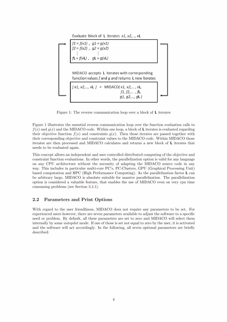
Figure 1: The reverse communication loop over a block of L iterates

Figure 1 illustrates the essential reverse communication loop over the function evaluation calls tof(x) and g(x) and the MIDACO code. Within one loop, a block of L iterates is evaluated regardingtheir objective function f(x) and constraints g(x). Then those iterates are passed together withtheir corresponding objective and constraint values to the MIDACO code. Within MIDACO thoseiterates are then processed and MIDACO calculates and returns a new block of L iterates thatneeds to be evaluated again.

This concept allows an independent and user controlled distributed computing of the objective andconstraint function evaluations. In other words, the parallelization option is valid for any languageon any CPU architecture without the necessity of adapting the MIDACO source code in anyway. This includes in particular multi-core PC’s, PC-Clusters, GPU (Graphical Processing Unit)based computation and HPC (High Performance Computing). As the parallelization factor L canbe arbitrary large, MIDACO is absolute suitable for massive parallelization. The parallelizationoption is considered a valuable feature, that enables the use of MIDACO even on very cpu timeconsuming problems (see Section 3.4.1).

2.2 Parameters and Print Options

With regard to the user friendliness, MIDACO does not require any parameters to be set. Forexperienced users however, there are seven parameters available to adjust the software to a specificneed or problem. By default, all these parameters are set to zero and MIDACO will select theminternally by some autopilot mode. If one of those is set not equal to zero by the user, it is activatedand the software will act accordingly. In the following, all seven optional parameters are brieflydescribed:

4

Seed - Initial seed for internal pseudo random number generator within MIDACO. The Seeddetermines the sequence of pseudo random numbers sampled by the generator. ThereforeMIDACO runs using an identical Seed, will produce exactly the same results (executedon the same computer under identical compiler conditions). As the Seed may be an arbitraryinteger greater or equal to zero, the user can easily generate (stochastically) differentruns, using a different Seed parameter. The advantage of a user specified random seed is,that promising runs can easily be reproduced by knowing the applied Seed parameter. Thisis in esp. useful, if a run must be stopped out of some reason and should be restarted again.

Qstart - This parameter allows the user to specify the quality of the starting point. IfQstart is set greater than 0, the initial population of iterates (also called ants)is sampled closely around the starting point. In particular, the standard deviationfor continuous variables is set to |xl − xu|/Qstart and the mean is set tothe corresponding dimension of the starting point. For integer variables thestandard deviation is set to max|yl − yu|/Qstart, 1/

√Qstart

to avoid a too tight sampling. The greater Qstart is selected, the moreclosely does MIDACO search around the starting point. This option is veryuseful to refine previously calculated solutions. It is important to note,that this option does not shrink the search space. The original boundsxl, yl and xu, yu are still valid, only the initial population of antsis specifically focused within these bounds.

Autostop - This parameter activates an internal stopping criteria for MIDACO. While it isrecommended, that the user will run MIDACO for a fixed time or evaluationbudget, this option allows the software to stop the optimization run by itself.Autostop defines the amount of internal restarts in sequence, that did not revealan improvement in the objective function value. The greater Autostop is selected,the higher the chance of global optimality, but also the longer the optimization run.As Autostop can be selected any integer greater or equal to zero, it gives the userthe freedom to compromise between global optimality and cpu run time to his or herspecific needs.

Oracle - This parameter specifies a user given oracle parameter Ω [21] to the penalty functionwithin MIDACO. If Oracle is selected not equal to zero, MIDACO will use the Oracleas long as a better feasible solution has been found. In that case the regular oracleupdate (see [21]) starts to take place. This option can be useful for problems withdifficult constraints where some background knowledge on the problem exists.

Ants - This parameter fixes the amount of iterates (also called ants) within a generation.This option can be useful to adapt MIDACO to expensive cpu time problems,or problems with many variables (e.g. more than hundred).

Kernel - This parameter fixes the kernel size in a generation used by the Gauss distributions.The Kernel parameter must be used in combination with the Ants parameter andis intended to make MIDACO more efficiently on specific problems.

Character - This parameter activates a specific set of MIDACO internal parameters specially tunedfor either purely continuous, purely combinatorial or mixed integer problems. If Characteris set to zero, MIDACO will select the according set of internal parameters solely based onthe problem dimensions n and nint. The intention of this option is to allow the user tomanually activate a different set, if a problem has a specific structure. For example, considera mixed integer problem with 98 continuous and 2 integer variables. In such a case it mightbe more promising to activate the internal Character for purely continuous, ratherthan the one for mixed integer, problems.

5

For the sake of a maximal portability and efficiency, the MIDACO Fortran77 and C source codedoes not include any printing commands by itself. Printing options are available by externalsubroutines freely distributed with example calls of MIDACO in different languages (see http://

www.midaco-solver.com/download.html). Those routines allows the user to specify the printingto his or her specific needs with high accuracy. The routines especially feature the option to printthe current best solution to a file in a user defined frequency. In other words, the user has access tothe current best solution vector at any time during the optimization process. This is an importantfeature for applications, that are executed over a long time horizon (where the run might getcorrupted and the solution would get lost otherwise).

3 Numerical Results

This section presents numerical results obtained by MIDACO on a set of 100 non-convex MINLPbenchmark problems from the open literature. The set of benchmark problems is provided inFortran by Schittkowski [15] and can freely be downloaded at

http://www.math.uni-bayreuth.de/~kschittkowski/mitp_coll.htm

Please note, that many of these problems are originally taken form the GAMS library MINLPlib [9].The dimension of these problems range between 2 and 100. The number of nonlinear constraintsrange between 0 to 54 with up to 17 equality constraints. The problems are either mixed integeror purely combinatorial problems. Their difficulty widely ranges from very easy to difficult. Inconclusion, this set provides a comprehensive variety of small to medium scaled MINLP problemsand allows a rigorous testing of software codes written in Fortran.

This section will first summarize already published results obtained by some deterministic SQP-based algorithms on the problem set. Then, numerical results by MIDACO are presented andcompared to the ones obtained by the SQP-based algorithms. Further numerical results investigatethe performance under consideration of its automatic stopping criteria. The impact of (massive)parallelization of the problem function calls is investigated in Section 3.4. An additional comparisonof MIDACO to the MINLP solvers BONMIN [4] and COUENNE [5] is performed on a subset of66 problems, which are provided in the GAMS library MINLPlib [9]. Finally a brief subsectionillustrates the black-box capabilities of MIDACO, by demonstrating the performance on some testproblems, which incorporate critical function properties.

All numerical results in this contribution refer to the Fortran77 version of MIDACO. The resultsin Section 3.2, Section 3.3 and Section 3.4 were computed by MIDACO version 3.0 on a computerwith an Intel(R) Xeon(R) E5640 CPU with 2.67GHz clock rate. The results in Section 3.5 andSection 3.6 were computed by MIDACO version 2.0 on a computer with an Intel(R) Core(TM) i7Q820 CPU with 1.73GHz clock rate. If not explicitly mentioned differently, MIDACO has beenused by its default parameters (see Section 2.2).

3.1 Performance of SQP-based Algorithms

In a recent study by Exler et al. [8] eight sophisticated implementations of SQP-based algorithmsfor MINLP were presented and evaluated on this set of 100 benchmarks. Table 1 contains essentialinformation (taken from Exler et al. [8], calculated on an Intel(R) Core(7) i7 processor with3.16GHz) on the performance of these eight algorithms. The abbreviations of Table 1 are asfollows:

Algorithm - Name of the SQP-based algorithm for MINLP used in Exler et al. [8]Optimal - Number of global (or best known) optimal solutions obtained out of 100 problemsFeasible - Number of feasible solutions obtained out of 100 problemsEvalmean - Average number of function evaluations over global optimal solved problemsTimemean - Average number of function evaluations over global optimal solved problems

6

http://www.midaco-solver.com/download.html

http://www.midaco-solver.com/download.html

http://www.math.uni-bayreuth.de/~kschittkowski/mitp_coll.htm

Table 1: Performance of SQP-based algorithms on 100 MINLP benchmarks presented in [8]Algorithm Optimal Feasible Evalmean Timemean

MISQP 89 100 500 0.39MISQP/bmod 71 100 340 0.20MISQP/fwd 81 100 396 0.11MISQP/rst0 69 99 241 0.14MISQPOA 91 100 1,093 0.65MISQPN 74 98 1,139 0.17MINLPB4/bin 92 100 1,787 30.91MINLPB4/int 88 94 218,881 4.11

The algorithms MISQP/bmod, MISQP/fwd and MISQP/rst0 represent different variants of thebasic-MISQP algorithm. The algorithms MISQPOA and MISQPN are enhanced by an Outer Ap-proximation method. The algorithms MINLPB4/bin and MINLPB4/int are enhanced by Branchand Bound. For detailed information on all algorithms consult Exler et al. [8]. Determining thesuccess of an algorithm in finding a global (or best known) optimal solution is done in Exler et al.[8] by the following criteria:

|f(x, y)− f(x∗, y∗)||f(x∗, y∗)|

< ε, (2)

where (x, y) is the (feasible) solution obtained by the algorithm, (x∗, y∗) is the best known solutionand ε is some tolerance. Wether a solution is feasible or not is dependent on the L∞-norm of thevector of constraint violations. A solution (x, y) is considered feasible, if:

‖g(x, y)‖∞ < acc, (3)

where acc is some accuracy. In Exler et al. [8] a tolerance of ε = 0.01 and an accuracy ofacc = 0.0001 were applied for the numerical results.

All SQP-based algorithms were started from a priori defined initial points given for every problemin the source code of the library by Schittkowski [15]. In Exler et al. [8] there is no investigationon the impact of these pre-defined initial points on the performance of the eight algorithms. Inother words, it is not known, if and how much the results would change, in case other (e.g. randominitial points) would have been used.

3.2 MIDACO Performance on 100 MINLP Benchmarks

Here numerical results obtained by MIDACO 3.0 for the set of 100 MINLP problems are presented.The same criteria for global (or best known) solutions and feasibility (illustrated in equation (2)and (3)) like in Exler et al. [8] is applied. For the test runs of MIDACO a tolerance of ε = 0.01and an accuracy of acc = 0.0001 was used, which are identical to those tolerances as used in Exleret al. [8]. In the following, the term global optimal solution will always refer to the best knownsolution provided in Schittkowski [15].

A critical aspect of MIDACO (and most stochastic algorithms) is the stopping criteria. For theresults in this section, there are two stopping criteria applied. Firstly, a maximal cpu time budgetof 300 seconds (5 minutes) for every test problem and secondly the success criteria for globaloptimality presented in equation (2). This means, in both cases MIDACO is stopped from outside,it does not stop by itself. In contrary to this, the SQP-based algorithms presented in Exler etal. [8] stop by themselves and the optimality criteria is checked afterwards. The internal stoppingcriteria of MIDACO, named Autostop, is investigated separately in Section 3.3.

As initial point random points are used that are stochastically generated for every individual testrun. Hence MIDACO does not make use of the pre-defined initial points provided in the library.As MIDACO is of stochastic nature, the full set of 100 problems is evaluated 10 times usinga different random seed (from 0 to 9) for the internal pseudo random number generator. Thisprocedure ensures objective conclusions on the robustness of the software.

7

Table 2 lists the results obtained by MIDACO by 10 runs with different Seed on the full set of100 problems. Besides the number of global optimal and feasible solutions, the average number offunction evaluation and time and the total required cpu time is reported. The abbreviations forTable 2 are as follows:

Seed - Initial seed for MIDACO’s internal pseudo random number generatorOptimal - Number of global optimal solutions obtained out of 100 problemsFeasible - Number of feasible solutions obtained out of 100 problemsEvalmean - Average number of function evaluation over global optimal solved problemsTimemean - Average cpu time (seconds) over global optimal solved problems

Table 2: MIDACO Performance on 100 MINLP BenchmarksSeed Optimal Feasible Evalmean Timemean

0 96 99 1,656,979 4.541 96 99 3,223,015 9.012 96 98 1,673,873 4.203 97 98 2,235,463 6.534 96 98 2,054,099 6.085 97 99 1,485,525 4.826 95 99 1,641,648 4.077 97 99 1,724,627 5.908 95 99 1,120,204 2.779 96 98 2,313,829 7.93

The results in Table 2 show a very robust MIDACO performance always obtaining between 95and 97 global optimal solutions and between 98 and 99 feasible solutions. The average amount offunction evaluation ranges between 1.5 and 3.2 million, while the average cpu time varies between2.77 to 9.01 seconds. Please note, that this implies that the MIDACO software is able to processmillions of iterates within seconds on a standard computer. Regarding the random seed, the bestrun was obtained for Seed = 5.

Comparing the results of Table 2 with the ones obtained by the SQP-based algorithms presented inTable 1, MIDACO robustly achieved a significantly higher percentage of global optimal solutionsthan any of the SQP-based algorithms (which range between 69 and 92 global optimal solutions). Infavor of MIDACO, this conclusion must further take into account, that the SQP-based algorithmswere started only one time from pre-defined initial points. MIDACO instead was not making useof the pre-defined initial points and was tested 10 times on the full library.

Regarding the number of function evaluation, MIDACO performs significantly more evaluationthan the SQP-based algorithms (which widely range between 241 and 218,881 evaluation). Thisresults is however expected, as stochastic algorithms like MIDACO are known to require muchmore evaluation than deterministic ones like SQP. In terms of cpu-time performance MIDACO isat least competitive with the SQP-based algorithms (which widely range between 0.11 and 30.91seconds). In favor of MIDACO, one has to further take into account, that the mean values forevaluation and cpu-time are calculated over 95 to 97 global solutions, while those of the SQP-basedalgorithms are calculated only over 69 to 92 global solutions.

3.3 The Automatic Stopping Criteria

The numerical results by MIDACO presented in Section 3.2 used exclusively external stoppingcriteria, in particular a maximal cpu time budget and the success in finding the global optimalsolution. In general it is difficult for most stochastic algorithms to decide by themselves, whento stop an optimization run. MIDACO is no exception and the missing of an accurate stoppingcriteria is considered a small disadvantage of the algorithm. In practice, it is recommended for

8

users to execute MIDACO with a maximal available time budget. This procedure ensures thehighest chance of global optimality.

Nevertheless, MIDACO offers the option of a heuristic stopping criteria based on the currentprogress of the algorithm. If the user activates the Autostop parameter (this is selecting it aninteger greater than zero, see Section 2.2), MIDACO will stop by itself, if a number of Autostopinternal restarts in sequence did not improve the best feasible solution. The algorithm will neverstop (even if Autostop is activated), if no feasible solution at all has been found so far. Thisstopping criteria is rather primitive, but in contrast to a fixed number of iterations and alike, ittakes into account the current progress of the algorithm.

A benefit of the Autostop parameter is that the user can scale this option to his or her specific needsby selecting either a small or a large value. A small value for Autostop has a higher probability tocause the algorithm to stop prematurely, but results in a faster runtime. A large value for Autostopwill result in a higher probability in finding the global optimal solution, but will also increase theruntime.

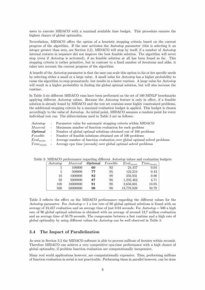
In Table 3 six different MIDACO runs have been performed on the set of 100 MINLP benchmarksapplying different Autostop values. Because the Autostop feature is only in effect, if a feasiblesolution is already found by MIDACO and the test set contains some highly constrained problems,the additional stopping criteria by a maximal evaluation budget is applied. This budget is chosenaccordingly to the value of Autostop. As initial point, MIDACO assumes a random point for everyindividual test run. The abbreviations used in Table 3 are as follows:

Autostop - Parameter value for automatic stopping criteria within MIDACOMaxeval - Maximum number of function evaluation for each problemOptimal - Number of global optimal solutions obtained out of 100 problemsFeasible - Number of feasible solutions obtained out of 100 problemsEvalmean - Average number of function evaluation over global optimal solved problemsTimemean - Average cpu time (seconds) over global optimal solved problems

Table 3: MIDACO performance regarding different Autostop values and evaluation budgetsAutostop Maxeval Optimal Feasible Evalmean Timemean

1 100000 60 92 24,457 0.045 500000 77 95 122,254 0.43

10 1000000 82 98 256,931 0.9050 5000000 87 98 1,232,462 4.71

100 10000000 91 98 2,656,601 10.05500 50000000 96 98 13,776,828 50.79

Table 3 reflects the effect on the MIDACO performance regarding the different values for theAutostop parameter. For Autostop = 1 a low rate of 60 global optimal solutions is found with anaverage of 24,457 evaluation and an average time of just 0.04 seconds. For Autostop = 500 a highrate of 96 global optimal solutions is obtained with an average of around 13,7 million evaluationand an average time of 50.79 seconds. The compromise between a fast runtime and a high rate ofglobal optimality by using different values for Autostop can be well observed in Table 3.

3.4 The Impact of Parallelization

As seen in Section 3.2 the MIDACO software is able to process millions of iterates within seconds.Therefore MIDACO can achieve a very competitive cpu-time performance with a high chance ofglobal optimality, if problem function evaluation are computationally inexpensive.

Many real world applications however, are computationally expensive. Thus, performing millionsof function evaluation in serial is not practicable. Performing them in parallel however, can be done

9

in a reasonable time, if an adequate cpu architecture is available. The parallelization option offeredby MIDACO is based on this idea. By (massively) parallelizing the problem function evaluation,even cpu time expensive problems become solvable by MIDACO in a reasonable time.

In the following, a series of experiments is performed, investigating the impact of the parallelizationfactor L (see Section 2.1) on the MIDACO performance on the same set of 100 MINLP problemsknown from above. A fixed budget of evaluation blocks is considered as budget for MIDACO. Ablock denotes here the amount of L iterates that are evaluated and passed to MIDACO within onereverse communication loop (see Figure 1). Regarding the computational time performance, theamount of blocks processed by MIDACO is directly comparable to the amount of serial processedfunction evaluation by an algorithm. For the experiment presented here, the problem function eval-uation of L iterates given in every block were executed in serial, rather than actually parallelized.As due to the reverse communication concept the function evaluation are completely independentof the MIDACO code, this makes absolutely no difference for MIDACO. Hence those experimentsonly simulate the impact of parallelization on the MIDACO performance. Note that nevertheless,the conclusions on the impact of an actual parallelization are absolute accurate and valid.

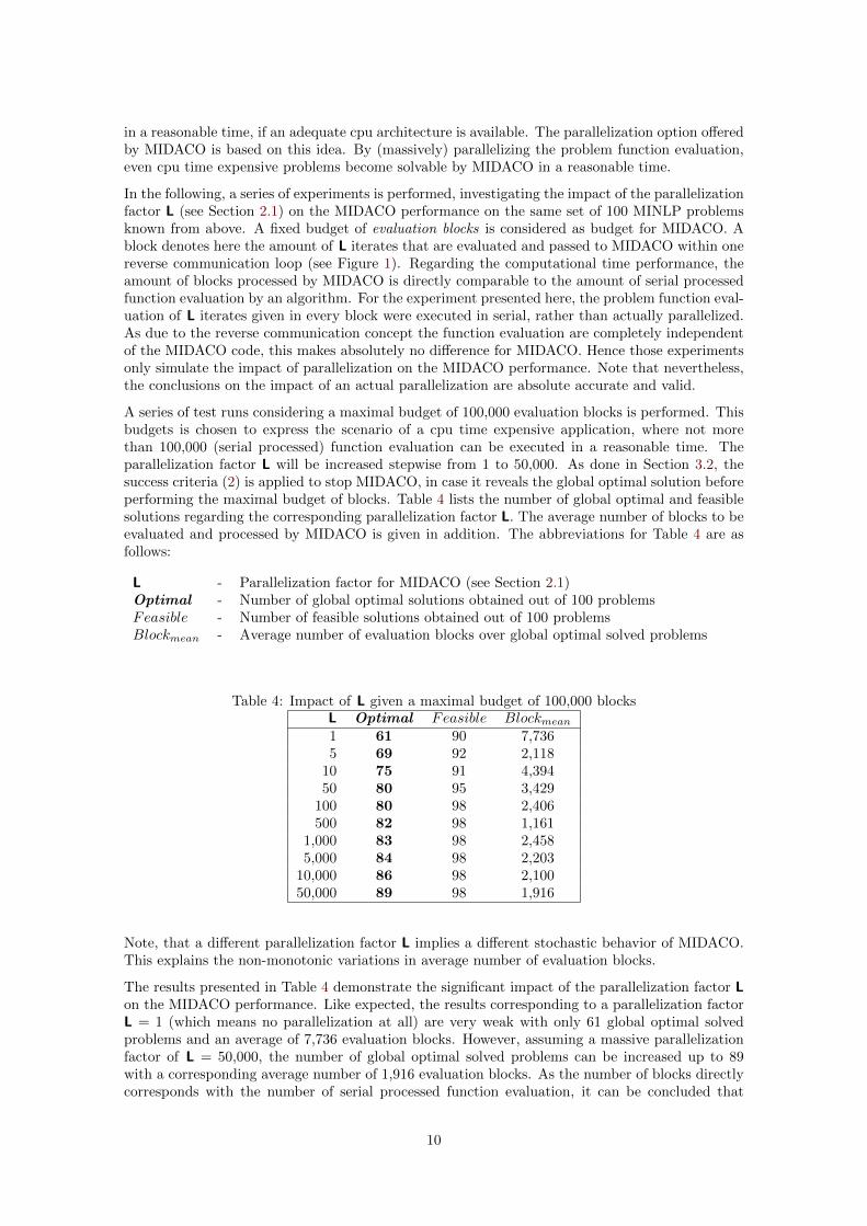
A series of test runs considering a maximal budget of 100,000 evaluation blocks is performed. Thisbudgets is chosen to express the scenario of a cpu time expensive application, where not morethan 100,000 (serial processed) function evaluation can be executed in a reasonable time. Theparallelization factor L will be increased stepwise from 1 to 50,000. As done in Section 3.2, thesuccess criteria (2) is applied to stop MIDACO, in case it reveals the global optimal solution beforeperforming the maximal budget of blocks. Table 4 lists the number of global optimal and feasiblesolutions regarding the corresponding parallelization factor L. The average number of blocks to beevaluated and processed by MIDACO is given in addition. The abbreviations for Table 4 are asfollows:

L - Parallelization factor for MIDACO (see Section 2.1)Optimal - Number of global optimal solutions obtained out of 100 problemsFeasible - Number of feasible solutions obtained out of 100 problemsBlockmean - Average number of evaluation blocks over global optimal solved problems

Table 4: Impact of L given a maximal budget of 100,000 blocksL Optimal Feasible Blockmean

1 61 90 7,7365 69 92 2,118

10 75 91 4,39450 80 95 3,429

100 80 98 2,406500 82 98 1,161

1,000 83 98 2,4585,000 84 98 2,203

10,000 86 98 2,10050,000 89 98 1,916

Note, that a different parallelization factor L implies a different stochastic behavior of MIDACO.This explains the non-monotonic variations in average number of evaluation blocks.

The results presented in Table 4 demonstrate the significant impact of the parallelization factor Lon the MIDACO performance. Like expected, the results corresponding to a parallelization factorL = 1 (which means no parallelization at all) are very weak with only 61 global optimal solvedproblems and an average of 7,736 evaluation blocks. However, assuming a massive parallelizationfactor of L = 50,000, the number of global optimal solved problems can be increased up to 89with a corresponding average number of 1,916 evaluation blocks. As the number of blocks directlycorresponds with the number of serial processed function evaluation, it can be concluded that

10

MIDACO can even be competitive with some of the SQP-based algorithms (see Table 1) in termsof function evaluation, if (massive) parallelization capabilities are available.

3.4.1 A Note on Computational Expensive Applications

As mentioned in the introduction, the high amount of function evaluation usually required bystochastic algorithms is often used as knock-out argument regarding their application on compu-tational expensive applications. In Section 3.4 the remedy of parallelization of the time costlyfunction evaluation was presented, which enables the use of MIDACO even on such costly appli-cations.

Here a small reflection on the nature of cpu time expensive applications and its consequences shouldbe undertaken. It is reasonable to assume, that if an evaluation of a function (depending on notmore than some hundred variables) is requiring a lot of computational effort, it is a complex func-tion. In esp. this means, the longer the computational evaluation time, the higher the complexity.Very complex functions are more likely to include critical properties such as high non-convexity,discontinuities, flat spots or even stochastic distortions.

Most deterministic approaches have great difficulties in dealing with such properties. Stochasticapproaches like MIDACO in contrary are mostly black-box optimizers and therefore capable to dealwell with such characteristics. As a consequence, the application of a stochastic approach exploiting(massive) parallelization seems to be a more reasonable and promising choice on computationalexpensive applications in general. However, in case the specific nature of a computational expensiveapplication is well known and a proper algorithm is available, this argument is not valid.

3.5 Comparison with BONMIN and COUENNE on GAMS benchmarks

In addition to the comparison of MIDACO to the set of SQP based MINLP solvers given in Section3.1, a further comparison to the established MINLP solvers BONMIN [4] and COUENNE [5] isgiven here. The solver BONMIN implements a variety of deterministic algorithms (in esp. Branch& Bound and Outer Approximation) and ensures global optimal solutions for convex problems,for non-convex MINLP problems it is a heuristic like MIDACO. The solver COUENNE is a pricewining software (COIN-OR Cup 2010, see [10]), based on a Branch & Bound algorithm and aims atfinding global optimal solutions even for non-convex MINLP problems. Both solvers are providedby the Computational Infrastructure for Operations Research (COIN-OR) and are distributedwithin the GAMS [11] environment. These solvers have been used here out of the box, withoutany attempt to specify or tune their parameters or settings. A subset of 66 instances from the 100MINLP benchmarks (see Table 9) is considered for evaluating purposes. This subset represent thoseproblems from the 100 MINLP benchmarks, that are originally taken from the GAMS MINLPlib[9] benchmark library. A cpu time budget of 300 seconds has been applied to all solvers for eachinstance as maximal time limit. In case of MIDACO the automatic stopping criteria (see Section3.3) was activated. A value of 50 was chosen for the Autostop parameter (see Table 3), whichseems to provide a good balance between solution quality and cpu-runtime, based on the resultsreported in Table 3. For the deterministic solvers BONMIN and COUENNE only one test runfor every problem was performed, using the pre-defined starting point from the GAMS MINLPlib.As MIDACO is a stochastic solver, 10 test runs were performed for every problem instance, usinga different random seed. MIDACO did not make use of pre-defined starting points and uses thelower bounds as starting point on all instances instead.

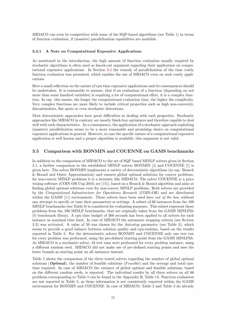
Table 5 shows the comparison of the three tested solvers regarding the number of global optimalsolutions (Optimal), the number of feasible solutions (Feasible) and the average and total cpu-time required. In case of MIDACO the variance of global optimal and feasible solutions, basedon the different random seeds, is reported. The individual results by all three solvers on all 66problems corresponding to Table 5 can be found in the Appendix B, Table 13. Function evaluationare not reported in Table 5, as those information is not consistently reported within the GAMSenvironment for BONMIN and COUENNE. In case of MIDACO, Table 2 and Table 3 do already

11

give evidence on the required function evaluation. All three solvers were tested on the samecomputer using an Intel(R) Core(TM) i7 Q820 CPU with 1.73GHz clock rate and 4GB RAM.

Table 5: Comparison of BONMIN, COUENNE and MIDACO on 66 MINLP benchmarksSolver Optimal Feasible T imeaver TimetotalBONMIN 49 64 17.99 1187.62COUENNE 48 64 40.36 2664.31MIDACO 51 ∼ 62 64 ∼ 65 31.41 2072.73

Based on the results in Table 5 it can be concluded, that MIDACO is fully competitive to the solversBONMIN and COUENNE regarding solution quality and cpu-runtime. MIDACO outperformsboth regarding the number of global optimal solutions found. In terms of cpu-runtime, MIDACOis able to outperform COUENNE, but is slower than BONMIN. Interpreting the results in Table5, one has to take further into account, that testing BONMIN and COUENNE within GAMSimplies a significant advantage for those solvers, as GAMS provides gradients to those algorithmsfor free (in terms of cpu-time). A further observation regarding the global optimality convergenceproof hold by COUENNE should be mentioned here. COUENNE reported falsely in 10 out of 66problems (this is 15.2%) a local solution as global optimal. This is assumingly due to numericaldifficulties and software bugs. However, this observation seems to put the numerical relevance ofa theoretical convergence proof, which MIDACO lacks of, into further perspective here.

3.6 Test Problems with Critical Function Properties

In order to demonstrate the black-box capabilities of MIDACO, five mixed integer test prob-lems, incorporating critical function properties, are considered here. These critical properties arenamely: stochastic noise, flat spots, non-convexity and non-differentiability. With exception tonon-convexity, these function properties are known to be very undesirable for most deterministicoptimization algorithms and are likely to be a knock-out argument for their usage. In contrastto this, MIDACO (based on a stochastic metaheuristic) can deal well with such critical functionproperties.

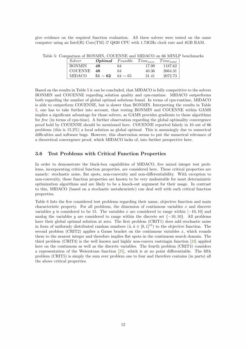
Table 6 lists the five considered test problems regarding their name, objective function and maincharacteristic property. For all problems, the dimension of continuous variables x and discretevariables y is considered to be 15. The variables x are considered to range within [−10, 10] andanalog the variables y are considered to range within the discrete set −10, 10. All problemshave their global optimal solution at zero. The first problem (CRIT1) does add stochastic noisein form of uniformly distributed random numbers (u, u ∈ [0, 1]15) to the objective function. Thesecond problem (CRIT2) applies a Gauss bracket on the continuous variables x, which roundsthem to the nearest integer and therefore implies flat spots in the continuous search domain. Thethird problem (CRIT3) is the well known and highly non-convex rastringin function [23] appliedhere on the continuous as well as the discrete variables. The fourth problem (CRIT4) considersa representation of the Weierstrass function [25], which is at no point differentiable. The fifthproblem (CRIT5) is simply the sum over problem one to four and therefore contains (in parts) allthe above critical properties.

12

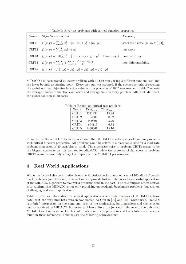
Table 6: Five test problems with critical function properties

Name Objective Function Property

CRIT1 f1(x, y) =∑15

i=1 x2i + |ui · xi|+ y2i + |ui · yi| stochastic noise (ui, ui ∈ [0, 1])

CRIT2 f2(x, y) =∑15

i=1[xi]2 + y2i flat spots

CRIT3 f3(x, y) = 150∑15

i=1 x2i − 10cos(2πxi) + y2i − 10cos(2πyi) non-convexity

CRIT4 f4(x, y) =∑15

i=1(xi∑10

k=12ksin(2kxi)

3k)2 non-differentiability

CRIT5 f5(x, y) = f1(x, y) + f2(x, y) + f3(x, y) + f4(x, y)

MIDACO has been tested on every problem with 10 test runs, using a different random seed andthe lower bounds as starting point. Every test run was stopped, if the success criteria of reachingthe global optimal objective function value with a precision of 10−4 was reached. Table 7 reportsthe average number of function evaluation and average time on every problem. MIDACO did reachthe global solution in all cases.

Table 7: Results on critical test problemsName Evalaver TimeaverCRIT1 3241433 15.24CRIT2 4608 0.02CRIT3 909501 5.26CRIT4 694113 6.34CRIT5 1436361 15.16

From the results in Table 7 it can be concluded, that MIDACO is well capable of handling problemswith critical function properties. All problems could be solved in a reasonable time for a moderateproblem dimension of 30 variables in total. The stochastic noise in problem CRIT4 seems to bethe biggest challenge on this test set for MIDACO, while the presence of flat spots in problemCRIT2 seem to have only a very low impact on the MIDACO performance.

4 Real World Applications

While the focus of this contribution is on the MIDACO performance on a set of 100 MINLP bench-mark problems (see Section 3), this section will provide further references to successful applicationof the MIDACO algorithm to real world problems done in the past. The sole purpose of this sectionis to confirm, that MIDACO is not only promising on academic benchmark problems, but also onchallenging real world applications.

Table 8 provides information on several applications where beta versions of MIDACO (pleasenote, that the very first beta version was named ACOmi in [19] and [20]) where used. Table 8lists brief information on the name and area of the application, its dimensions and the solutionquality obtained by MIDACO. For every problem a literature (or web-) reference to the publishedMIDACO solution is given. Further information on the applications and the solutions can also befound in those references. Table 8 uses the following abbreviations:

13

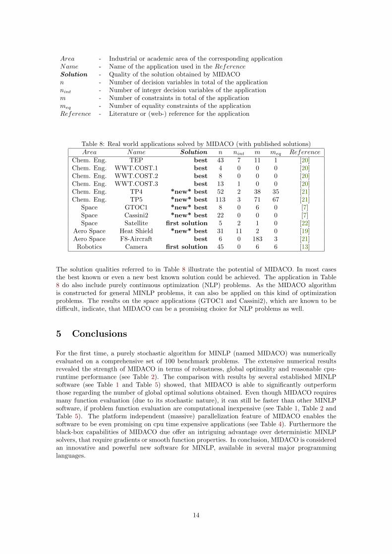
Area - Industrial or academic area of the corresponding applicationName - Name of the application used in the ReferenceSolution - Quality of the solution obtained by MIDACOn - Number of decision variables in total of the applicationnint - Number of integer decision variables of the applicationm - Number of constraints in total of the applicationmeq - Number of equality constraints of the applicationReference - Literature or (web-) reference for the application

Table 8: Real world applications solved by MIDACO (with published solutions)Area Name Solution n nint m meq Reference

Chem. Eng. TEP best 43 7 11 1 [20]Chem. Eng. WWT.COST.1 best 4 0 0 0 [20]Chem. Eng. WWT.COST.2 best 8 0 0 0 [20]Chem. Eng. WWT.COST.3 best 13 1 0 0 [20]Chem. Eng. TP4 *new* best 52 2 38 35 [21]Chem. Eng. TP5 *new* best 113 3 71 67 [21]

Space GTOC1 *new* best 8 0 6 0 [7]Space Cassini2 *new* best 22 0 0 0 [7]Space Satellite first solution 5 2 1 0 [22]

Aero Space Heat Shield *new* best 31 11 2 0 [19]Aero Space F8-Aircraft best 6 0 183 3 [21]Robotics Camera first solution 45 0 6 6 [13]

The solution qualities referred to in Table 8 illustrate the potential of MIDACO. In most casesthe best known or even a new best known solution could be achieved. The application in Table8 do also include purely continuous optimization (NLP) problems. As the MIDACO algorithmis constructed for general MINLP problems, it can also be applied on this kind of optimizationproblems. The results on the space applications (GTOC1 and Cassini2), which are known to bedifficult, indicate, that MIDACO can be a promising choice for NLP problems as well.

5 Conclusions

For the first time, a purely stochastic algorithm for MINLP (named MIDACO) was numericallyevaluated on a comprehensive set of 100 benchmark problems. The extensive numerical resultsrevealed the strength of MIDACO in terms of robustness, global optimality and reasonable cpu-runtime performance (see Table 2). The comparison with results by several established MINLPsoftware (see Table 1 and Table 5) showed, that MIDACO is able to significantly outperformthose regarding the number of global optimal solutions obtained. Even though MIDACO requiresmany function evaluation (due to its stochastic nature), it can still be faster than other MINLPsoftware, if problem function evaluation are computational inexpensive (see Table 1, Table 2 andTable 5). The platform independent (massive) parallelization feature of MIDACO enables thesoftware to be even promising on cpu time expensive applications (see Table 4). Furthermore theblack-box capabilities of MIDACO due offer an intriguing advantage over deterministic MINLPsolvers, that require gradients or smooth function properties. In conclusion, MIDACO is consideredan innovative and powerful new software for MINLP, available in several major programminglanguages.

14

Acknowledgments

The authors would like to thank K. Schittkowski, O. Exler and T. Lehmann for generously pro-viding the test set of MINLP benchmarks and many supportive help. Special thanks go to K.Schittkowski for inspiring important implementation features like the reverse communication andthe parallelization option for MIDACO. The development has been supported by the project ”Non-linear mixed-integer-based Optimisation Technique for Space Applications” (ESTEC/Contract No.21943/08/NL/ST) co-funded by ESA Networking Partnership Initiative, Astrium Limited (Steve-nage, UK) and the School of Mathematics, University of Birmingham, UK.

6 Appendix A

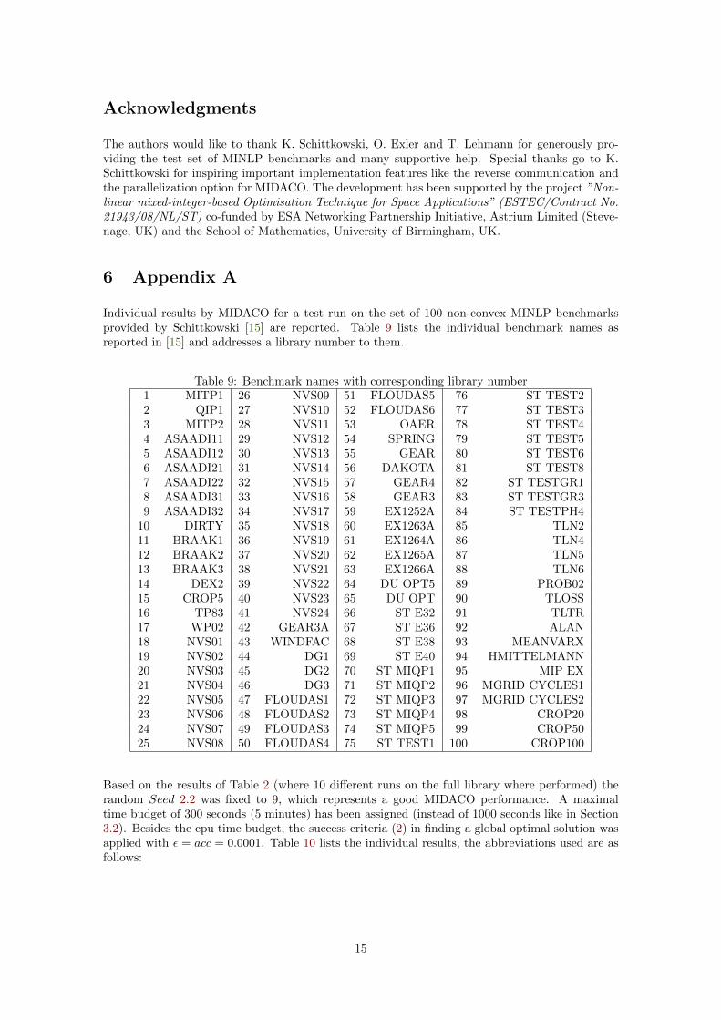
Individual results by MIDACO for a test run on the set of 100 non-convex MINLP benchmarksprovided by Schittkowski [15] are reported. Table 9 lists the individual benchmark names asreported in [15] and addresses a library number to them.

Table 9: Benchmark names with corresponding library number1 MITP1 26 NVS09 51 FLOUDAS5 76 ST TEST22 QIP1 27 NVS10 52 FLOUDAS6 77 ST TEST33 MITP2 28 NVS11 53 OAER 78 ST TEST44 ASAADI11 29 NVS12 54 SPRING 79 ST TEST55 ASAADI12 30 NVS13 55 GEAR 80 ST TEST66 ASAADI21 31 NVS14 56 DAKOTA 81 ST TEST87 ASAADI22 32 NVS15 57 GEAR4 82 ST TESTGR18 ASAADI31 33 NVS16 58 GEAR3 83 ST TESTGR39 ASAADI32 34 NVS17 59 EX1252A 84 ST TESTPH4

10 DIRTY 35 NVS18 60 EX1263A 85 TLN211 BRAAK1 36 NVS19 61 EX1264A 86 TLN412 BRAAK2 37 NVS20 62 EX1265A 87 TLN513 BRAAK3 38 NVS21 63 EX1266A 88 TLN614 DEX2 39 NVS22 64 DU OPT5 89 PROB0215 CROP5 40 NVS23 65 DU OPT 90 TLOSS16 TP83 41 NVS24 66 ST E32 91 TLTR17 WP02 42 GEAR3A 67 ST E36 92 ALAN18 NVS01 43 WINDFAC 68 ST E38 93 MEANVARX19 NVS02 44 DG1 69 ST E40 94 HMITTELMANN20 NVS03 45 DG2 70 ST MIQP1 95 MIP EX21 NVS04 46 DG3 71 ST MIQP2 96 MGRID CYCLES122 NVS05 47 FLOUDAS1 72 ST MIQP3 97 MGRID CYCLES223 NVS06 48 FLOUDAS2 73 ST MIQP4 98 CROP2024 NVS07 49 FLOUDAS3 74 ST MIQP5 99 CROP5025 NVS08 50 FLOUDAS4 75 ST TEST1 100 CROP100

Based on the results of Table 2 (where 10 different runs on the full library where performed) therandom Seed 2.2 was fixed to 9, which represents a good MIDACO performance. A maximaltime budget of 300 seconds (5 minutes) has been assigned (instead of 1000 seconds like in Section3.2). Besides the cpu time budget, the success criteria (2) in finding a global optimal solution wasapplied with ε = acc = 0.0001. Table 10 lists the individual results, the abbreviations used are asfollows:

15

Flag - Symbol indicating a local (-), false (x) or better (o) solutionNr. - MINLP problem number from the libraryEval - Number of function evaluation used by MIDACOTime - Cpu time in seconds used by MIDACOn - Number of decision variables in total of the problemnint - Number of integer decision variables of the problemm - Number of constraints in total of the problemmeq - Number of equality constraints of the problemf(x∗, y∗) - Global (or best known) optimal objective function valuef(x, y) - Best (feasible) objective function value obtained by MIDACOV iolation - Constraint violation measured as L∞-norm over all violations

16

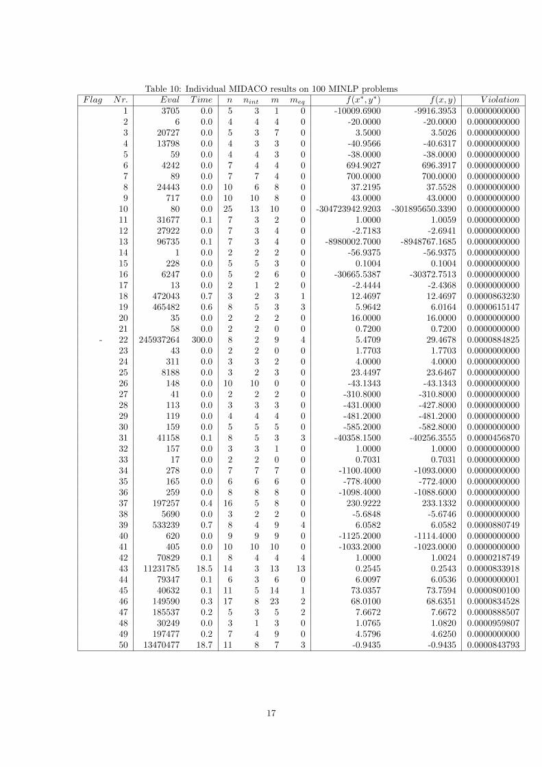
Table 10: Individual MIDACO results on 100 MINLP problemsFlag Nr. Eval T ime n nint m meq f(x∗, y∗) f(x, y) V iolation

1 3705 0.0 5 3 1 0 -10009.6900 -9916.3953 0.00000000002 6 0.0 4 4 4 0 -20.0000 -20.0000 0.00000000003 20727 0.0 5 3 7 0 3.5000 3.5026 0.00000000004 13798 0.0 4 3 3 0 -40.9566 -40.6317 0.00000000005 59 0.0 4 4 3 0 -38.0000 -38.0000 0.00000000006 4242 0.0 7 4 4 0 694.9027 696.3917 0.00000000007 89 0.0 7 7 4 0 700.0000 700.0000 0.00000000008 24443 0.0 10 6 8 0 37.2195 37.5528 0.00000000009 717 0.0 10 10 8 0 43.0000 43.0000 0.0000000000

10 80 0.0 25 13 10 0 -304723942.9203 -301895650.3390 0.000000000011 31677 0.1 7 3 2 0 1.0000 1.0059 0.000000000012 27922 0.0 7 3 4 0 -2.7183 -2.6941 0.000000000013 96735 0.1 7 3 4 0 -8980002.7000 -8948767.1685 0.000000000014 1 0.0 2 2 2 0 -56.9375 -56.9375 0.000000000015 228 0.0 5 5 3 0 0.1004 0.1004 0.000000000016 6247 0.0 5 2 6 0 -30665.5387 -30372.7513 0.000000000017 13 0.0 2 1 2 0 -2.4444 -2.4368 0.000000000018 472043 0.7 3 2 3 1 12.4697 12.4697 0.000086323019 465482 0.6 8 5 3 3 5.9642 6.0164 0.000061514720 35 0.0 2 2 2 0 16.0000 16.0000 0.000000000021 58 0.0 2 2 0 0 0.7200 0.7200 0.0000000000

- 22 245937264 300.0 8 2 9 4 5.4709 29.4678 0.000088482523 43 0.0 2 2 0 0 1.7703 1.7703 0.000000000024 311 0.0 3 3 2 0 4.0000 4.0000 0.000000000025 8188 0.0 3 2 3 0 23.4497 23.6467 0.000000000026 148 0.0 10 10 0 0 -43.1343 -43.1343 0.000000000027 41 0.0 2 2 2 0 -310.8000 -310.8000 0.000000000028 113 0.0 3 3 3 0 -431.0000 -427.8000 0.000000000029 119 0.0 4 4 4 0 -481.2000 -481.2000 0.000000000030 159 0.0 5 5 5 0 -585.2000 -582.8000 0.000000000031 41158 0.1 8 5 3 3 -40358.1500 -40256.3555 0.000045687032 157 0.0 3 3 1 0 1.0000 1.0000 0.000000000033 17 0.0 2 2 0 0 0.7031 0.7031 0.000000000034 278 0.0 7 7 7 0 -1100.4000 -1093.0000 0.000000000035 165 0.0 6 6 6 0 -778.4000 -772.4000 0.000000000036 259 0.0 8 8 8 0 -1098.4000 -1088.6000 0.000000000037 197257 0.4 16 5 8 0 230.9222 233.1332 0.000000000038 5690 0.0 3 2 2 0 -5.6848 -5.6746 0.000000000039 533239 0.7 8 4 9 4 6.0582 6.0582 0.000088074940 620 0.0 9 9 9 0 -1125.2000 -1114.4000 0.000000000041 405 0.0 10 10 10 0 -1033.2000 -1023.0000 0.000000000042 70829 0.1 8 4 4 4 1.0000 1.0024 0.000021874943 11231785 18.5 14 3 13 13 0.2545 0.2543 0.000083391844 79347 0.1 6 3 6 0 6.0097 6.0536 0.000000000145 40632 0.1 11 5 14 1 73.0357 73.7594 0.000080010046 149590 0.3 17 8 23 2 68.0100 68.6351 0.000083452847 185537 0.2 5 3 5 2 7.6672 7.6672 0.000088850748 30249 0.0 3 1 3 0 1.0765 1.0820 0.000095980749 197477 0.2 7 4 9 0 4.5796 4.6250 0.000000000050 13470477 18.7 11 8 7 3 -0.9435 -0.9435 0.0000843793

17

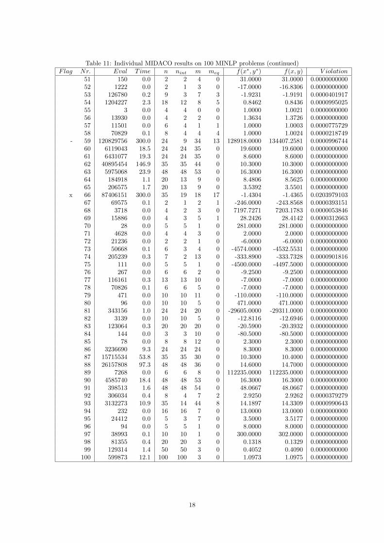
Table 11: Individual MIDACO results on 100 MINLP problems (continued)Flag Nr. Eval T ime n nint m meq f(x∗, y∗) f(x, y) V iolation

51 150 0.0 2 2 4 0 31.0000 31.0000 0.000000000052 1222 0.0 2 1 3 0 -17.0000 -16.8306 0.000000000053 126780 0.2 9 3 7 3 -1.9231 -1.9191 0.000040191754 1204227 2.3 18 12 8 5 0.8462 0.8436 0.000099502555 3 0.0 4 4 0 0 1.0000 1.0021 0.000000000056 13930 0.0 4 2 2 0 1.3634 1.3726 0.000000000057 11501 0.0 6 4 1 1 1.0000 1.0003 0.000077572958 70829 0.1 8 4 4 4 1.0000 1.0024 0.0000218749

- 59 120829756 300.0 24 9 34 13 128918.0000 134407.2581 0.000099674460 6119043 18.5 24 24 35 0 19.6000 19.6000 0.000000000061 6431077 19.3 24 24 35 0 8.6000 8.6000 0.000000000062 40895454 146.9 35 35 44 0 10.3000 10.3000 0.000000000063 5975068 23.9 48 48 53 0 16.3000 16.3000 0.000000000064 184918 1.1 20 13 9 0 8.4806 8.5625 0.000000000065 206575 1.7 20 13 9 0 3.5392 3.5501 0.0000000000

x 66 87406151 300.0 35 19 18 17 -1.4304 -1.4365 0.020397910367 69575 0.1 2 1 2 1 -246.0000 -243.8568 0.000039315168 3718 0.0 4 2 3 0 7197.7271 7203.1783 0.000005384669 15886 0.0 4 3 5 1 28.2426 28.4142 0.000031266370 28 0.0 5 5 1 0 281.0000 281.0000 0.000000000071 4628 0.0 4 4 3 0 2.0000 2.0000 0.000000000072 21236 0.0 2 2 1 0 -6.0000 -6.0000 0.000000000073 50668 0.1 6 3 4 0 -4574.0000 -4532.5531 0.000000000074 205239 0.3 7 2 13 0 -333.8900 -333.7328 0.000090181675 111 0.0 5 5 1 0 -4500.0000 -4497.5000 0.000000000076 267 0.0 6 6 2 0 -9.2500 -9.2500 0.000000000077 116161 0.3 13 13 10 0 -7.0000 -7.0000 0.000000000078 70826 0.1 6 6 5 0 -7.0000 -7.0000 0.000000000079 471 0.0 10 10 11 0 -110.0000 -110.0000 0.000000000080 96 0.0 10 10 5 0 471.0000 471.0000 0.000000000081 343156 1.0 24 24 20 0 -29605.0000 -29311.0000 0.000000000082 3139 0.0 10 10 5 0 -12.8116 -12.6946 0.000000000083 123064 0.3 20 20 20 0 -20.5900 -20.3932 0.000000000084 144 0.0 3 3 10 0 -80.5000 -80.5000 0.000000000085 78 0.0 8 8 12 0 2.3000 2.3000 0.000000000086 3236690 9.3 24 24 24 0 8.3000 8.3000 0.000000000087 15715534 53.8 35 35 30 0 10.3000 10.4000 0.000000000088 26157808 97.3 48 48 36 0 14.6000 14.7000 0.000000000089 7268 0.0 6 6 8 0 112235.0000 112235.0000 0.000000000090 4585740 18.4 48 48 53 0 16.3000 16.3000 0.000000000091 398513 1.6 48 48 54 0 48.0667 48.0667 0.000000000092 306034 0.4 8 4 7 2 2.9250 2.9262 0.000037927993 3132273 10.9 35 14 44 8 14.1897 14.3309 0.000099064394 232 0.0 16 16 7 0 13.0000 13.0000 0.000000000095 24412 0.0 5 3 7 0 3.5000 3.5177 0.000000000096 94 0.0 5 5 1 0 8.0000 8.0000 0.000000000097 38993 0.1 10 10 1 0 300.0000 302.0000 0.000000000098 81355 0.4 20 20 3 0 0.1318 0.1329 0.000000000099 129314 1.4 50 50 3 0 0.4052 0.4090 0.0000000000

100 599873 12.1 100 100 3 0 1.0973 1.0975 0.0000000000

18

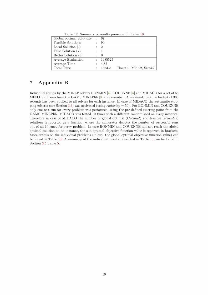
Table 12: Summary of results presented in Table 10Global optimal Solutions : 97Feasible Solutions : 99Local Solution (-) : 2False Solution (x) : 1Better Solution (o) : 0Average Evaluation : 1485525Average Time : 4.82Total Time : 1363.2 [Hour: 0, Min:22, Sec:43]

7 Appendix B

Individual results by the MINLP solvers BONMIN [4], COUENNE [5] and MIDACO for a set of 66MINLP problems form the GAMS MINLPlib [9] are presented. A maximal cpu time budget of 300seconds has been applied to all solvers for each instance. In case of MIDACO the automatic stop-ping criteria (see Section 3.3) was activated (using Autostop = 50). For BONMIN and COUENNEonly one test run for every problem was performed, using the pre-defined starting point from theGAMS MINLPlib. MIDACO was tested 10 times with a different random seed on every instance.Therefore in case of MIDACO the number of global optimal (Optimal) and feasible (Feasible)solutions is reported as a fraction, where the numerator denotes the number of successful runsout of all 10 runs, for every problem. In case BONMIN and COUENNE did not reach the globaloptimal solution on an instance, the sub-optimal objective function value is reported in brackets.More details on the individual problems (in esp. the global optimal objective function value) canbe found in Table 10. A summary of the individual results presented in Table 13 can be found inSection 3.5 Table 5.

19

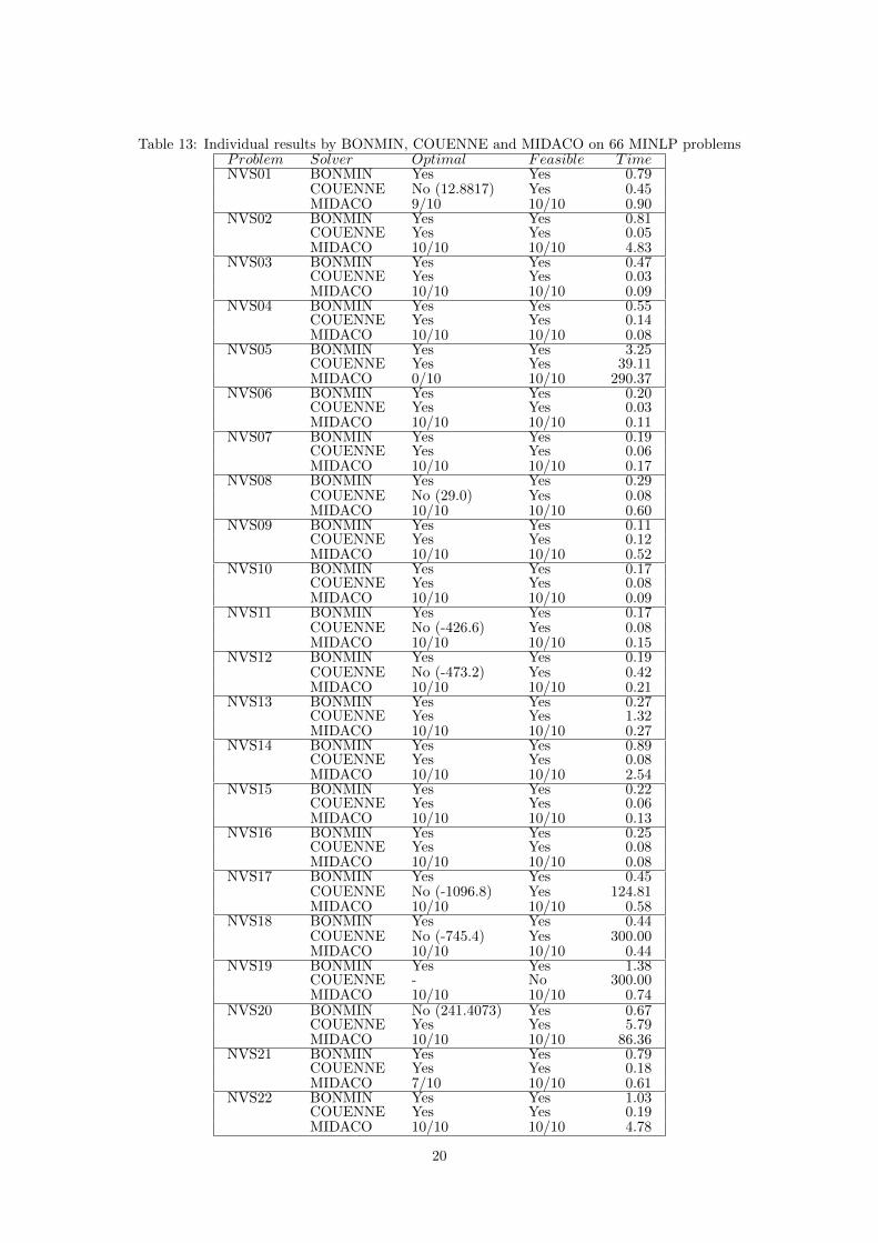
Table 13: Individual results by BONMIN, COUENNE and MIDACO on 66 MINLP problemsProblem Solver Optimal Feasible T imeNVS01 BONMIN Yes Yes 0.79

COUENNE No (12.8817) Yes 0.45MIDACO 9/10 10/10 0.90

NVS02 BONMIN Yes Yes 0.81COUENNE Yes Yes 0.05MIDACO 10/10 10/10 4.83






NVS08 BONMIN Yes Yes 0.29COUENNE No (29.0) Yes 0.08MIDACO 10/10 10/10 0.60



NVS11 BONMIN Yes Yes 0.17COUENNE No (-426.6) Yes 0.08MIDACO 10/10 10/10 0.15








NVS19 BONMIN Yes Yes 1.38COUENNE - No 300.00MIDACO 10/10 10/10 0.74

NVS20 BONMIN No (241.4073) Yes 0.67COUENNE Yes Yes 5.79MIDACO 10/10 10/10 86.36



20

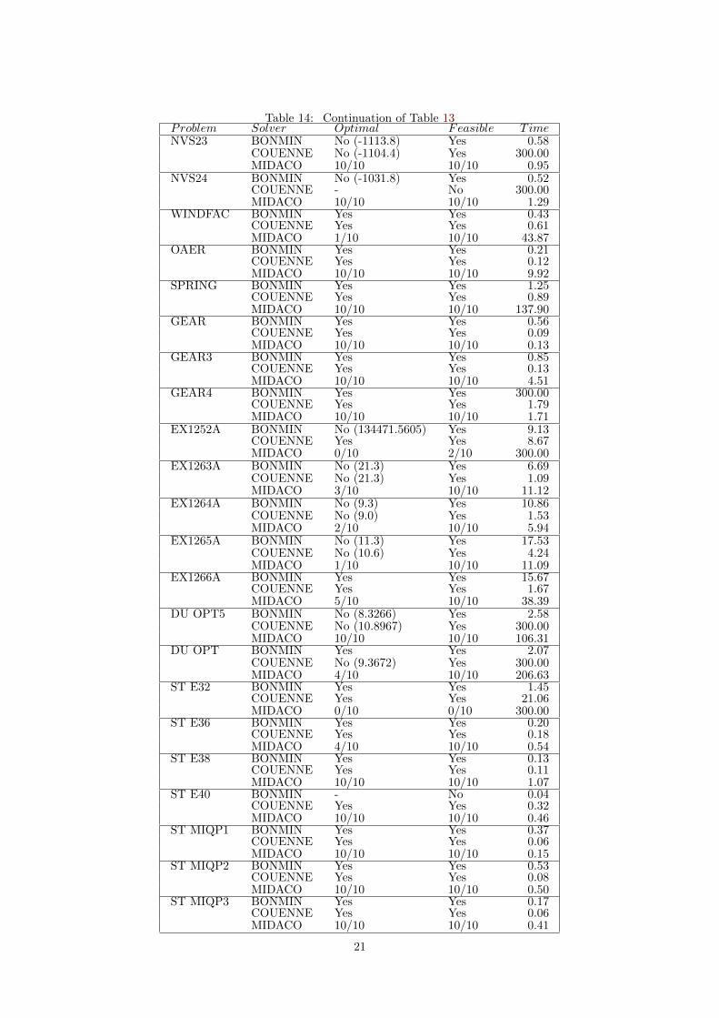
Table 14: Continuation of Table 13Problem Solver Optimal Feasible T imeNVS23 BONMIN No (-1113.8) Yes 0.58

COUENNE No (-1104.4) Yes 300.00MIDACO 10/10 10/10 0.95

NVS24 BONMIN No (-1031.8) Yes 0.52COUENNE - No 300.00MIDACO 10/10 10/10 1.29

WINDFAC BONMIN Yes Yes 0.43COUENNE Yes Yes 0.61MIDACO 1/10 10/10 43.87

OAER BONMIN Yes Yes 0.21COUENNE Yes Yes 0.12MIDACO 10/10 10/10 9.92

SPRING BONMIN Yes Yes 1.25COUENNE Yes Yes 0.89MIDACO 10/10 10/10 137.90

GEAR BONMIN Yes Yes 0.56COUENNE Yes Yes 0.09MIDACO 10/10 10/10 0.13

GEAR3 BONMIN Yes Yes 0.85COUENNE Yes Yes 0.13MIDACO 10/10 10/10 4.51

GEAR4 BONMIN Yes Yes 300.00COUENNE Yes Yes 1.79MIDACO 10/10 10/10 1.71

EX1252A BONMIN No (134471.5605) Yes 9.13COUENNE Yes Yes 8.67MIDACO 0/10 2/10 300.00

EX1263A BONMIN No (21.3) Yes 6.69COUENNE No (21.3) Yes 1.09MIDACO 3/10 10/10 11.12



EX1266A BONMIN Yes Yes 15.67COUENNE Yes Yes 1.67MIDACO 5/10 10/10 38.39

DU OPT5 BONMIN No (8.3266) Yes 2.58COUENNE No (10.8967) Yes 300.00MIDACO 10/10 10/10 106.31

DU OPT BONMIN Yes Yes 2.07COUENNE No (9.3672) Yes 300.00MIDACO 4/10 10/10 206.63

ST E32 BONMIN Yes Yes 1.45COUENNE Yes Yes 21.06MIDACO 0/10 0/10 300.00



ST E40 BONMIN - No 0.04COUENNE Yes Yes 0.32MIDACO 10/10 10/10 0.46

ST MIQP1 BONMIN Yes Yes 0.37COUENNE Yes Yes 0.06MIDACO 10/10 10/10 0.15



21

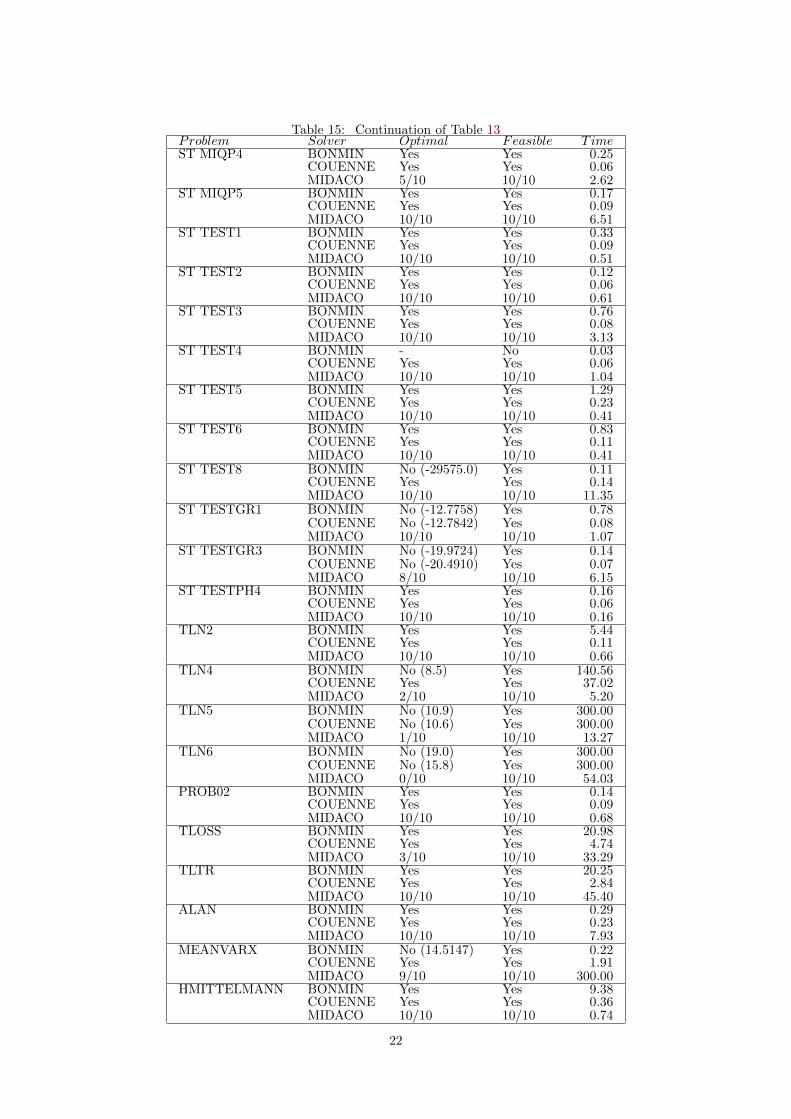
Table 15: Continuation of Table 13Problem Solver Optimal Feasible T imeST MIQP4 BONMIN Yes Yes 0.25

COUENNE Yes Yes 0.06MIDACO 5/10 10/10 2.62


ST TEST1 BONMIN Yes Yes 0.33COUENNE Yes Yes 0.09MIDACO 10/10 10/10 0.51



ST TEST4 BONMIN - No 0.03COUENNE Yes Yes 0.06MIDACO 10/10 10/10 1.04



ST TEST8 BONMIN No (-29575.0) Yes 0.11COUENNE Yes Yes 0.14MIDACO 10/10 10/10 11.35

ST TESTGR1 BONMIN No (-12.7758) Yes 0.78COUENNE No (-12.7842) Yes 0.08MIDACO 10/10 10/10 1.07

ST TESTGR3 BONMIN No (-19.9724) Yes 0.14COUENNE No (-20.4910) Yes 0.07MIDACO 8/10 10/10 6.15

ST TESTPH4 BONMIN Yes Yes 0.16COUENNE Yes Yes 0.06MIDACO 10/10 10/10 0.16

TLN2 BONMIN Yes Yes 5.44COUENNE Yes Yes 0.11MIDACO 10/10 10/10 0.66

TLN4 BONMIN No (8.5) Yes 140.56COUENNE Yes Yes 37.02MIDACO 2/10 10/10 5.20

TLN5 BONMIN No (10.9) Yes 300.00COUENNE No (10.6) Yes 300.00MIDACO 1/10 10/10 13.27

TLN6 BONMIN No (19.0) Yes 300.00COUENNE No (15.8) Yes 300.00MIDACO 0/10 10/10 54.03

PROB02 BONMIN Yes Yes 0.14COUENNE Yes Yes 0.09MIDACO 10/10 10/10 0.68

TLOSS BONMIN Yes Yes 20.98COUENNE Yes Yes 4.74MIDACO 3/10 10/10 33.29

TLTR BONMIN Yes Yes 20.25COUENNE Yes Yes 2.84MIDACO 10/10 10/10 45.40

ALAN BONMIN Yes Yes 0.29COUENNE Yes Yes 0.23MIDACO 10/10 10/10 7.93

MEANVARX BONMIN No (14.5147) Yes 0.22COUENNE Yes Yes 1.91MIDACO 9/10 10/10 300.00

HMITTELMANN BONMIN Yes Yes 9.38COUENNE Yes Yes 0.36MIDACO 10/10 10/10 0.74

22

References

[1] G.E.P. Box and M.E. Muller, A Note on the Generation of Random Normal Deviates, Ann.Math. Statist. 29(2) (1958), pp. 610–611

[2] C. Blum, Ant colony optimization: Introduction and recent trends, Phys. Life Rev. 2(4) (2005),pp. 353 – 373

[3] M.R. Bussieck and S. Vigerske, MINLP Solver Software, J.J. Cochran, L.A. Cox, P. Ke-skinocak, J.P. Kharoufeh and J.C. Smith, Wiley Encyclopedia of Operations Research andManagement Science, John Wiley and Sons, Inc., New York, 2010

[4] COIN-OR (Project Manager P. Bonami), Basic Open-source Nonlinear Mixed INteger pro-gramming ; software available at http://www.coin-or.org/Bonmin/

[5] COIN-OR (Project Manager P. Belotti), Convex Over and Under ENvelopes for NonlinearEstimation; software available at http://www.coin-or.org/Couenne/

[6] M. Dorigo and T. Stuetzle, Ant Colony Optimization, MIT Press, Cambridge, 2004

[7] European Space Agency (ESA) and Advanced Concepts Team (ACT), GTOP Database -Global Optimisation Trajectory Problems and Solutions; software available at http://www.

esa.int/gsp/ACT/inf/op/globopt.htm

[8] O. Exler, T. Lehmann and K. Schittkowski, A Comparative Study of SQP-Type Algorithms forNonlinear and Nonconvex Mixed-Integer Optimization, preprint (2010), submitted for publi-cation. Available at http://www.ai7.uni-bayreuth.de/minlp_comp_study.htm

[9] GAMS MINLPlib - A collection of Mixed Integer Nonlinear Programming models. Washington,DC, USA; software available at http://www.gamsworld.org/minlp/minlplib.htm

[10] Matt Saltzman: Informs 2010 Annual Meeting Blogposts. Austin, Texas, USA. Available athttp://meetings2.informs.org/Austin2010/blog/?p=88

[11] GAMS (General Algebraic Modeling System). Washington, DC, USA; software available athttp://www.gams.com/

[12] I.E. Grossmann, Review of Nonlinear Mixed-Integer and Disjunctive Programming Techniques,Optim. Eng. 3(3) (2002), pp. 227–252

[13] M. Hanel, S. Kuhn, D. Henrich, L. Grune, and J. Pannek, Optimal Camera Placement tomeasure Distances Conservativly Regarding Static and Dynamic Obstacles, preprint (2011).Available at http://arxiv.org/abs/1105.3270

[14] G. Marsaglia, Xorshift RNGs, J. Stat. Softw. 8(14) (2003), pp. 1–6

[15] K. Schittkowski, A Collection of 100 Test Problems for Nonlinear Mixed-Integer Programmingin Fortran (User Guide), Report, Department of Computer Science, University of Bayreuth,Bayreuth, 2009

[16] K. Schittkowski, NLPQLP - A Fortran implementation of a sequential quadratic programmingalgorithm with distributed and non-monotone line search (User Guide), Report, Departmentof Computer Science, University of Bayreuth, Bayreuth, 2009

[17] K. Socha, ACO for Continuous and Mixed-Variable Optimization, Lect. Notes Comput. Sc.Vol. 3172, Springer, Berlin, 2004, pp. 25–36

[18] K. Socha and M. Dorigo, Ant colony optimization for continuous domains, Eur. J. Oper. Res.85(2008), pp. 1155–1173

[19] M. Schluter, J.A. Egea and J.R. Banga, Extended antcolony optimization for non-convex mixedinteger nonlinear programming, Comput. Oper. Res. 36(7) (2009), pp. 2217–2229

23

http://www.coin-or.org/Bonmin/

http://www.coin-or.org/Couenne/

http://www.esa.int/gsp/ACT/inf/op/globopt.htm

http://www.esa.int/gsp/ACT/inf/op/globopt.htm

http://www.ai7.uni-bayreuth.de/minlp_comp_study.htm

http://www.gamsworld.org/minlp/minlplib.htm

http://meetings2.informs.org/Austin2010/blog/?p=88

http://www.gams.com/

http://arxiv.org/abs/1105.3270

[20] M. Schluter, J.A. Egea, L.T. Antelo, A.A. Alonso and J.R. Banga, An extended ant colonyoptimization algorithm for integrated process and control system design, Ind. Eng. Chem.48(14) (2009), pp. 6723–6738

[21] M. Schluter and M. Gerdts, The Oracle Penalty Method, J. Global Optim. 47(2) (2010), pp.293–325

[22] A.T. Takano and B.G. Marchand, Optimal Constellation Design for Space Based Situa-tional Awareness Applications, Astrodynamics Specialists Conference (AAS/AIAA), PaperNo. AAS11-543, Girdwood, AK, 2011. Available at http://www.ae.utexas.edu/~marchand/AAS11-543.pdf

[23] A. Torn and A. Zilinskas, Global Optimization, Lect. Notes Comput. Sc. Vol. 350, Springer,1989

[24] Z. Ugray, L. Lasdon, J. Plummer, F. Glover, J. Kelly and R. Marti, Scatter Search and LocalNLP Solvers: A Multistart Framework for Global Optimization, Informs J. Comput. 19(3)(2007), pp. 328–340

[25] K. Weierstrass, Abhandlungen aus der Functionenlehre, Julius Springer, Berlin (1886)

24

http://www.ae.utexas.edu/~marchand/AAS11-543.pdf

http://www.ae.utexas.edu/~marchand/AAS11-543.pdf

a numerical study of midaco on 100 minlp...

Documents