a riemann-hilbert problem for the moisil-teodorescu system · the moisil-teodorescu system. this...
TRANSCRIPT
Universitätsverlag Potsdam
Alexander Polkovnikov | Nikolai Tarkhanov
A Riemann-Hilbert Problem for the Moisil-Teodorescu System
Preprints des Instituts für Mathematik der Universität Potsdam 6 (2017) 3


Preprints des Instituts für Mathematik der Universität Potsdam

Preprints des Instituts für Mathematik der Universität Potsdam 6 (2017) 3
Alexander Polkovnikov | Nikolai Tarkhanov
A Riemann-Hilbert Problem for the Moisil-Teodorescu System
Universitätsverlag Potsdam
Bibliografische Information der Deutschen Nationalbibliothek Die Deutsche Nationalbibliothek verzeichnet diese Publikation in der Deutschen Nationalbibliografie; detaillierte bibliografische Daten sind im Internet über http://dnb.dnb.de abrufbar. Universitätsverlag Potsdam 2017 http://verlag.ub.uni-potsdam.de/ Am Neuen Palais 10, 14469 Potsdam Tel.: +49 (0)331 977 2533 / Fax: 2292 E-Mail: [email protected] Die Schriftenreihe Preprints des Instituts für Mathematik der Universität Potsdam wird herausgegeben vom Institut für Mathematik der Universität Potsdam. ISSN (online) 2193-6943 Kontakt: Institut für Mathematik Karl-Liebknecht-Straße 24/25 14476 Potsdam Tel.: +49 (0)331 977 1499 WWW: http://www.math.uni-potsdam.de Titelabbildungen: 1. Karla Fritze | Institutsgebäude auf dem Campus Neues Palais 2. Nicolas Curien, Wendelin Werner | Random hyperbolic triangulation Published at: http://arxiv.org/abs/1105.5089 Das Manuskript ist urheberrechtlich geschützt. Online veröffentlicht auf dem Publikationsserver der Universität Potsdam URL https://publishup.uni-potsdam.de/opus4-ubp/frontdoor/index/index/docId/39703 URN urn:nbn:de:kobv:517-opus4-397036 http://nbn-resolving.de/urn:nbn:de:kobv:517-opus4-397036
A RIEMANN-HILBERT PROBLEM
FOR THE MOISIL-TEODORESCU SYSTEM
ALEXANDER POLKOVNIKOV AND NIKOLAI TARKHANOV
Abstract. In a bounded domain with smooth boundary in R3 we consider
the stationary Maxwell equations for a function u with values in R3 subject
to a nonhomogeneous condition (u, v)x = u0 on the boundary, where v is a
given vector field and u0 a function on the boundary. We specify this problem
within the framework of the Riemann-Hilbert boundary value problems for
the Moisil-Teodorescu system. This latter is proved to satisfy the Shapiro-
Lopaniskij condition if an only if the vector v is at no point tangent to the
boundary. The Riemann-Hilbert problem for the Moisil-Teodorescu system
fails to possess an adjoint boundary value problem with respect to the Green
formula, which satisfies the Shapiro-Lopatinskij condition. We develop the
construction of Green formula to get a proper concept of adjoint boundaryvalue problem.
Contents
Introduction 2
Part 1. The Riemann-Hilbert boundary value problem 31. Setting of the problem 32. The main theorem on elliptic boundary value problems 43. Applications to the Riemann-Hilbert problem 6
Part 2. The Moisil-Teodoresco system 114. The Green formula 125. A calculation for the Moisil-Teodoresco system 156. The Fredholm property 17
Part 3. Boundary Fourier method 187. Hardy spaces 188. The Cauchy problem 209. Operator-theoretic foundations 22
Part 4. Application to the Riemann-Hilbert problem 2510. The Fischer-Riesz equations 2511. Regularisation of solutions 2712. Solvability of elliptic boundary value problems 29References 31
Date: April 12, 2017.
2010 Mathematics Subject Classification. Primary 35F45; Secondary 35J56, 47N20.
Key words and phrases. Dirac operator, Riemann-Hilbert problem, Fredholm operators.
1
2 A. POLKOVNIKOV AND N. TARKHANOV
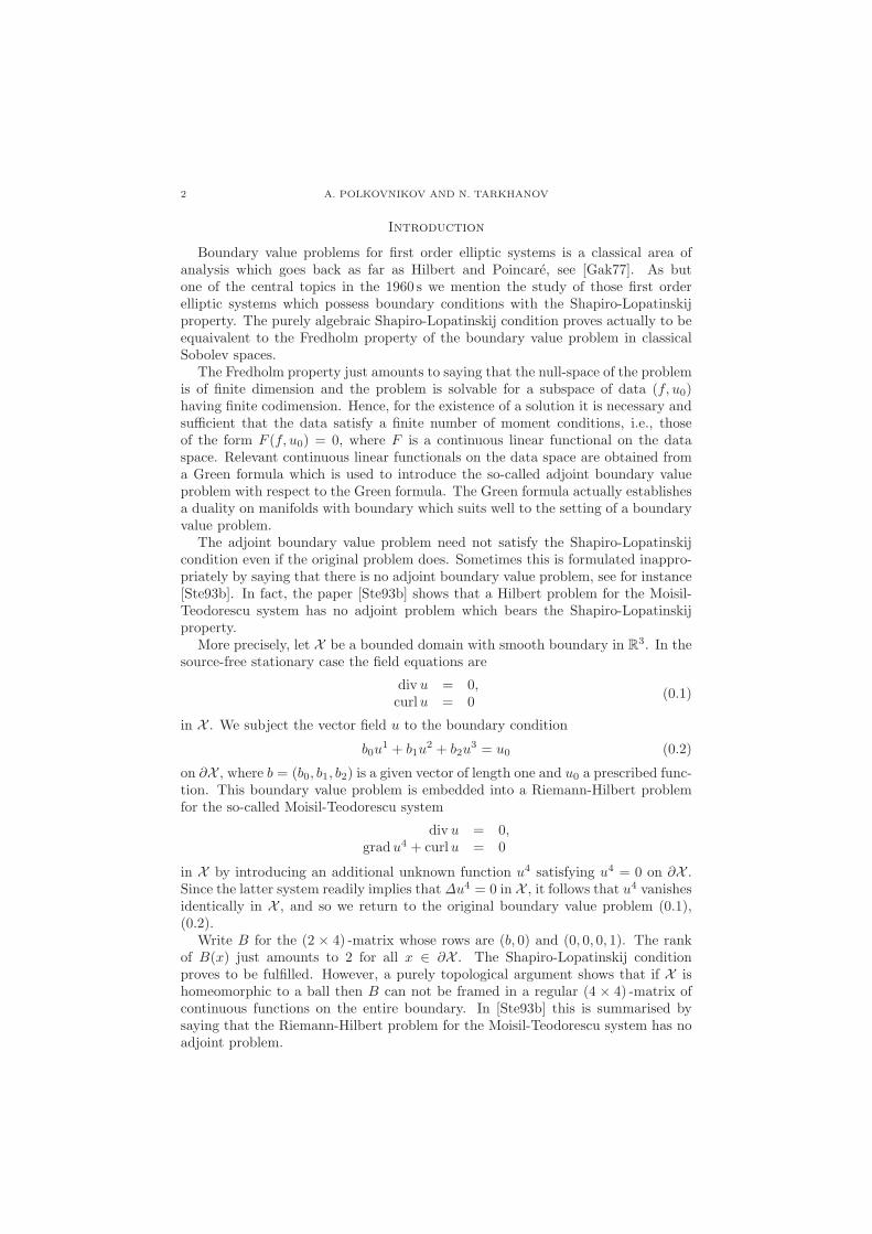
Introduction
Boundary value problems for first order elliptic systems is a classical area ofanalysis which goes back as far as Hilbert and Poincare, see [Gak77]. As butone of the central topics in the 1960 s we mention the study of those first orderelliptic systems which possess boundary conditions with the Shapiro-Lopatinskijproperty. The purely algebraic Shapiro-Lopatinskij condition proves actually to beequaivalent to the Fredholm property of the boundary value problem in classicalSobolev spaces.
The Fredholm property just amounts to saying that the null-space of the problemis of finite dimension and the problem is solvable for a subspace of data (f, u0)having finite codimension. Hence, for the existence of a solution it is necessary andsufficient that the data satisfy a finite number of moment conditions, i.e., thoseof the form F (f, u0) = 0, where F is a continuous linear functional on the dataspace. Relevant continuous linear functionals on the data space are obtained froma Green formula which is used to introduce the so-called adjoint boundary valueproblem with respect to the Green formula. The Green formula actually establishesa duality on manifolds with boundary which suits well to the setting of a boundaryvalue problem.
The adjoint boundary value problem need not satisfy the Shapiro-Lopatinskijcondition even if the original problem does. Sometimes this is formulated inappro-priately by saying that there is no adjoint boundary value problem, see for instance[Ste93b]. In fact, the paper [Ste93b] shows that a Hilbert problem for the Moisil-Teodorescu system has no adjoint problem which bears the Shapiro-Lopatinskijproperty.
More precisely, let X be a bounded domain with smooth boundary in R3. In the
source-free stationary case the field equations are
div u = 0,curlu = 0
(0.1)
in X . We subject the vector field u to the boundary condition
b0u1 + b1u
2 + b2u3 = u0 (0.2)
on ∂X , where b = (b0, b1, b2) is a given vector of length one and u0 a prescribed func-tion. This boundary value problem is embedded into a Riemann-Hilbert problemfor the so-called Moisil-Teodorescu system
div u = 0,gradu4 + curlu = 0
in X by introducing an additional unknown function u4 satisfying u4 = 0 on ∂X .Since the latter system readily implies thatΔu4 = 0 in X , it follows that u4 vanishesidentically in X , and so we return to the original boundary value problem (0.1),(0.2).
Write B for the (2 × 4) -matrix whose rows are (b, 0) and (0, 0, 0, 1). The rankof B(x) just amounts to 2 for all x ∈ ∂X . The Shapiro-Lopatinskij conditionproves to be fulfilled. However, a purely topological argument shows that if X ishomeomorphic to a ball then B can not be framed in a regular (4 × 4) -matrix ofcontinuous functions on the entire boundary. In [Ste93b] this is summarised bysaying that the Riemann-Hilbert problem for the Moisil-Teodorescu system has noadjoint problem.
A RIEMANN-HILBERT PROBLEM 3
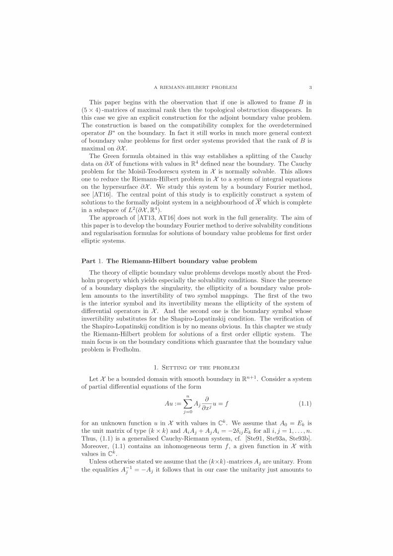
This paper begins with the observation that if one is allowed to frame B in(5 × 4) -matrices of maximal rank then the topological obstruction disappears. Inthis case we give an explicit construction for the adjoint boundary value problem.The construction is based on the compatibility complex for the overdeterminedoperator B∗ on the boundary. In fact it still works in much more general contextof boundary value problems for first order systems provided that the rank of B ismaximal on ∂X .
The Green formula obtained in this way establishes a splitting of the Cauchydata on ∂X of functions with values in R
4 defined near the boundary. The Cauchyproblem for the Moisil-Teodorescu system in X is normally solvable. This allowsone to reduce the Riemann-Hilbert problem in X to a system of integral equationson the hypersurface ∂X . We study this system by a boundary Fourier method,see [AT16]. The central point of this study is to explicitly construct a system ofsolutions to the formally adjoint system in a neighbourhood of X which is completein a subspace of L2(∂X ,R4).
The approach of [AT13, AT16] does not work in the full generality. The aim ofthis paper is to develop the boundary Fourier method to derive solvability conditionsand regularisation formulas for solutions of boundary value problems for first orderelliptic systems.
Part 1. The Riemann-Hilbert boundary value problem
The theory of elliptic boundary value problems develops mostly about the Fred-holm property which yields especially the solvability conditions. Since the presenceof a boundary displays the singularity, the ellipticity of a boundary value prob-lem amounts to the invertibility of two symbol mappings. The first of the twois the interior symbol and its invertibility means the ellipticity of the system ofdifferential operators in X . And the second one is the boundary symbol whoseinvertibility substitutes for the Shapiro-Lopatinskij condition. The verification ofthe Shapiro-Lopatinskij condition is by no means obvious. In this chapter we studythe Riemann-Hilbert problem for solutions of a first order elliptic system. Themain focus is on the boundary conditions which guarantee that the boundary valueproblem is Fredholm.
1. Setting of the problem
Let X be a bounded domain with smooth boundary in Rn+1. Consider a system
of partial differential equations of the form
Au :=n∑
j=0
Aj∂
∂xju = f (1.1)
for an unknown function u in X with values in Ck. We assume that A0 = Ek is
the unit matrix of type (k × k) and AiAj +AjAi = −2δijEk for all i, j = 1, . . . , n.Thus, (1.1) is a generalised Cauchy-Riemann system, cf. [Ste91, Ste93a, Ste93b].Moreover, (1.1) contains an inhomogeneous term f , a given function in X withvalues in C
k.Unless otherwise stated we assume that the (k×k) -matrices Aj are unitary. From
the equalities A−1j = −Aj it follows that in our case the unitarity just amounts to
4 A. POLKOVNIKOV AND N. TARKHANOV
saying that
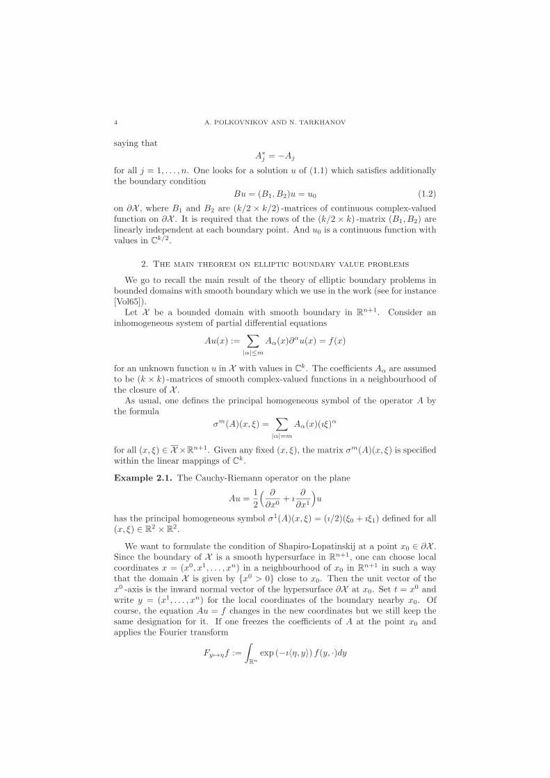
A∗j = −Aj
for all j = 1, . . . , n. One looks for a solution u of (1.1) which satisfies additionallythe boundary condition
Bu = (B1, B2)u = u0 (1.2)
on ∂X , where B1 and B2 are (k/2 × k/2) -matrices of continuous complex-valuedfunction on ∂X . It is required that the rows of the (k/2 × k) -matrix (B1, B2) arelinearly independent at each boundary point. And u0 is a continuous function withvalues in C
k/2.
2. The main theorem on elliptic boundary value problems
We go to recall the main result of the theory of elliptic boundary problems inbounded domains with smooth boundary which we use in the work (see for instance[Vol65]).
Let X be a bounded domain with smooth boundary in Rn+1. Consider an
inhomogeneous system of partial differential equations
Au(x) :=∑
|α|≤m
Aα(x)∂αu(x) = f(x)
for an unknown function u in X with values in Ck. The coefficients Aα are assumed
to be (k × k) -matrices of smooth complex-valued functions in a neighbourhood ofthe closure of X .
As usual, one defines the principal homogeneous symbol of the operator A bythe formula
σm(A)(x, ξ) =∑
|α|=m
Aα(x)(ıξ)α
for all (x, ξ) ∈ X ×Rn+1. Given any fixed (x, ξ), the matrix σm(A)(x, ξ) is specified
within the linear mappings of Ck.
Example 2.1. The Cauchy-Riemann operator on the plane
Au =1
2
( ∂
∂x0+ ı
∂
∂x1
)u
has the principal homogeneous symbol σ1(A)(x, ξ) = (ı/2)(ξ0 + ıξ1) defined for all(x, ξ) ∈ R
2 × R2.
We want to formulate the condition of Shapiro-Lopatinskij at a point x0 ∈ ∂X .Since the boundary of X is a smooth hypersurface in R
n+1, one can choose localcoordinates x = (x0, x1, . . . , xn) in a neighbourhood of x0 in R
n+1 in such a waythat the domain X is given by {x0 > 0} close to x0. Then the unit vector of thex0 -axis is the inward normal vector of the hypersurface ∂X at x0. Set t = x0 andwrite y = (x1, . . . , xn) for the local coordinates of the boundary nearby x0. Ofcourse, the equation Au = f changes in the new coordinates but we still keep thesame designation for it. If one freezes the coefficients of A at the point x0 andapplies the Fourier transform
Fy �→ηf :=
∫Rn
exp (−ı〈η, y〉) f(y, ·)dy
A RIEMANN-HILBERT PROBLEM 5
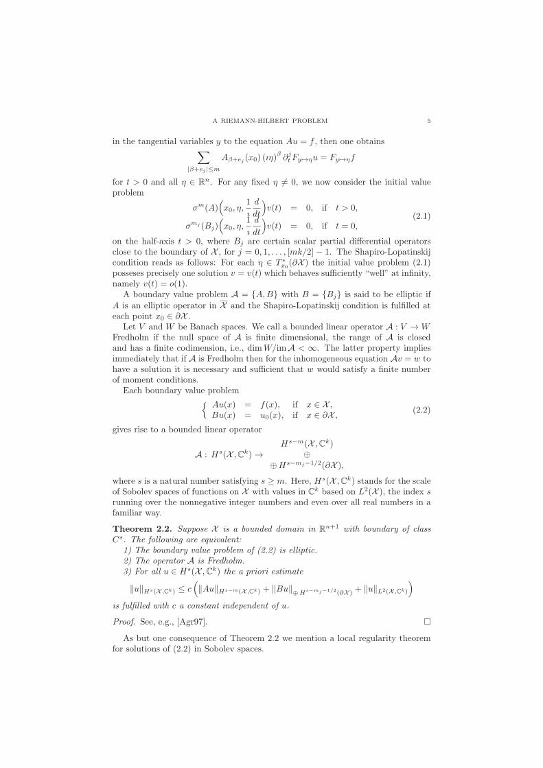
in the tangential variables y to the equation Au = f , then one obtains∑|β+ej |≤m
Aβ+ej (x0) (ıη)β∂jtFy �→ηu = Fy �→ηf
for t > 0 and all η ∈ Rn. For any fixed η �= 0, we now consider the initial value
problem
σm(A)(x0, η,
1
ı
d
dt
)v(t) = 0, if t > 0,
σmj (Bj)(x0, η,
1
ı
d
dt
)v(t) = 0, if t = 0,
(2.1)
on the half-axis t > 0, where Bj are certain scalar partial differential operatorsclose to the boundary of X , for j = 0, 1, . . . , [mk/2] − 1. The Shapiro-Lopatinskijcondition reads as follows: For each η ∈ T ∗
x0(∂X ) the initial value problem (2.1)
posseses precisely one solution v = v(t) which behaves sufficiently “well” at infinity,namely v(t) = o(1).
A boundary value problem A = {A,B} with B = {Bj} is said to be elliptic if
A is an elliptic operator in X and the Shapiro-Lopatinskij condition is fulfilled ateach point x0 ∈ ∂X .
Let V and W be Banach spaces. We call a bounded linear operator A : V → WFredholm if the null space of A is finite dimensional, the range of A is closedand has a finite codimension, i.e., dimW/imA < ∞. The latter property impliesimmediately that if A is Fredholm then for the inhomogeneous equation Av = w tohave a solution it is necessary and sufficient that w would satisfy a finite numberof moment conditions.
Each boundary value problem{ Au(x) = f(x), if x ∈ X ,Bu(x) = u0(x), if x ∈ ∂X ,
(2.2)
gives rise to a bounded linear operator
A : Hs(X ,Ck) →Hs−m(X ,Ck)
⊕⊕Hs−mj−1/2(∂X ),
where s is a natural number satisfying s ≥ m. Here, Hs(X ,Ck) stands for the scaleof Sobolev spaces of functions on X with values in C
k based on L2(X ), the index srunning over the nonnegative integer numbers and even over all real numbers in afamiliar way.
Theorem 2.2. Suppose X is a bounded domain in Rn+1 with boundary of class
Cs. The following are equivalent:1) The boundary value problem of (2.2) is elliptic.2) The operator A is Fredholm.3) For all u ∈ Hs(X ,Ck) the a priori estimate
‖u‖Hs(X ,Ck) ≤ c(‖Au‖Hs−m(X ,Ck) + ‖Bu‖⊕Hs−mj−1/2(∂X )
+ ‖u‖L2(X ,Ck)
)is fulfilled with c a constant independent of u.
Proof. See, e.g., [Agr97]. �
As but one consequence of Theorem 2.2 we mention a local regularity theoremfor solutions of (2.2) in Sobolev spaces.
6 A. POLKOVNIKOV AND N. TARKHANOV
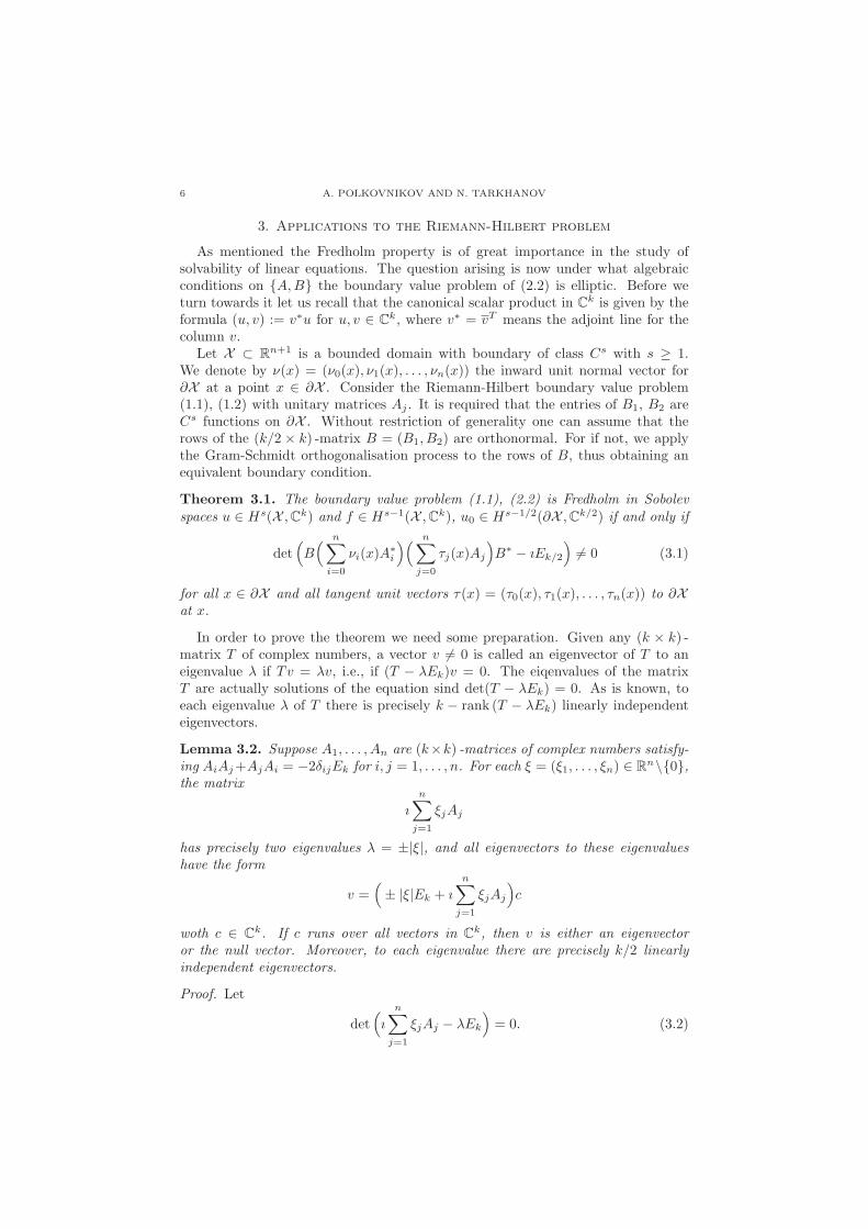
3. Applications to the Riemann-Hilbert problem
As mentioned the Fredholm property is of great importance in the study ofsolvability of linear equations. The question arising is now under what algebraicconditions on {A,B} the boundary value problem of (2.2) is elliptic. Before weturn towards it let us recall that the canonical scalar product in C
k is given by theformula (u, v) := v∗u for u, v ∈ C
k, where v∗ = vT means the adjoint line for thecolumn v.
Let X ⊂ Rn+1 is a bounded domain with boundary of class Cs with s ≥ 1.
We denote by ν(x) = (ν0(x), ν1(x), . . . , νn(x)) the inward unit normal vector for∂X at a point x ∈ ∂X . Consider the Riemann-Hilbert boundary value problem(1.1), (1.2) with unitary matrices Aj . It is required that the entries of B1, B2 areCs functions on ∂X . Without restriction of generality one can assume that therows of the (k/2 × k) -matrix B = (B1, B2) are orthonormal. For if not, we applythe Gram-Schmidt orthogonalisation process to the rows of B, thus obtaining anequivalent boundary condition.
Theorem 3.1. The boundary value problem (1.1), (2.2) is Fredholm in Sobolevspaces u ∈ Hs(X ,Ck) and f ∈ Hs−1(X ,Ck), u0 ∈ Hs−1/2(∂X ,Ck/2) if and only if
det(B( n∑
i=0
νi(x)A∗i
)( n∑j=0
τj(x)Aj
)B∗ − ıEk/2
)�= 0 (3.1)
for all x ∈ ∂X and all tangent unit vectors τ(x) = (τ0(x), τ1(x), . . . , τn(x)) to ∂Xat x.
In order to prove the theorem we need some preparation. Given any (k × k) -matrix T of complex numbers, a vector v �= 0 is called an eigenvector of T to aneigenvalue λ if Tv = λv, i.e., if (T − λEk)v = 0. The eiqenvalues of the matrixT are actually solutions of the equation sind det(T − λEk) = 0. As is known, toeach eigenvalue λ of T there is precisely k − rank (T − λEk) linearly independenteigenvectors.
Lemma 3.2. Suppose A1, . . . , An are (k×k) -matrices of complex numbers satisfy-ing AiAj+AjAi = −2δijEk for i, j = 1, . . . , n. For each ξ = (ξ1, . . . , ξn) ∈ R
n\{0},the matrix
ın∑
j=1
ξjAj
has precisely two eigenvalues λ = ±|ξ|, and all eigenvectors to these eigenvalueshave the form
v =(± |ξ|Ek + ı
n∑j=1
ξjAj
)c
woth c ∈ Ck. If c runs over all vectors in C
k, then v is either an eigenvectoror the null vector. Moreover, to each eigenvalue there are precisely k/2 linearlyindependent eigenvectors.
Proof. Let
det(ı
n∑j=1
ξjAj − λEk
)= 0. (3.2)
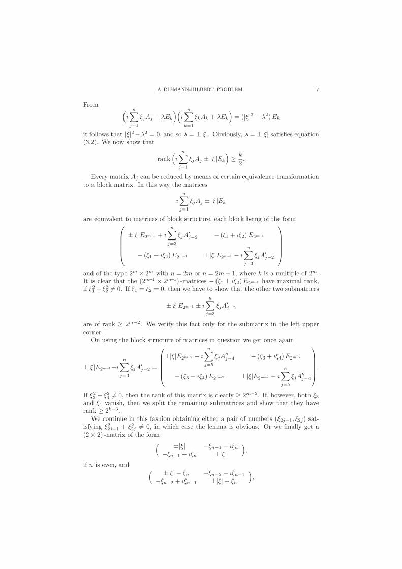
A RIEMANN-HILBERT PROBLEM 7
From (ı
n∑j=1
ξjAj − λEk
)(ı
n∑k=1
ξkAk + λEk
)= (|ξ|2 − λ2)Ek
it follows that |ξ|2−λ2 = 0, and so λ = ±|ξ|. Obviously, λ = ±|ξ| satisfies equation(3.2). We now show that
rank(ı
n∑j=1
ξjAj ± |ξ|Ek
)≥ k
2.
Every matrix Aj can be reduced by means of certain equivalence transformationto a block matrix. In this way the matrices
ı
n∑j=1
ξjAj ± |ξ|Ek
are equivalent to matrices of block structure, each block being of the form⎛⎜⎜⎜⎜⎝
±|ξ|E2m−1 + ın∑
j=3
ξjA′j−2 − (ξ1 + ıξ2)E2m−1
− (ξ1 − ıξ2)E2m−1 ±|ξ|E2m−1 − ı
n∑j=3
ξjA′j−2
⎞⎟⎟⎟⎟⎠
and of the type 2m × 2m with n = 2m or n = 2m+ 1, where k is a multiple of 2m.It is clear that the (2m−1 × 2m−1) -matrices − (ξ1 ± ıξ2)E2m−1 have maximal rank,if ξ21 + ξ22 �= 0. If ξ1 = ξ2 = 0, then we have to show that the other two submatrices
±|ξ|E2m−1 ± ı
n∑j=3
ξjA′j−2
are of rank ≥ 2m−2. We verify this fact only for the submatrix in the left uppercorner.
On using the block structure of matrices in question we get once again
±|ξ|E2m−1+ı
n∑j=3
ξjA′j−2 =
⎛⎜⎜⎜⎜⎝±|ξ|E2m−2 + ı
n∑j=5
ξjA′′j−4 − (ξ3 + ıξ4)E2m−2
− (ξ3 − ıξ4)E2m−2 ±|ξ|E2m−2 − ı
n∑j=5
ξjA′′j−4
⎞⎟⎟⎟⎟⎠ .
If ξ23 + ξ24 �= 0, then the rank of this matrix is clearly ≥ 2m−2. If, however, both ξ3and ξ4 vanish, then we split the remaining submatrices and show that they haverank ≥ 2k−3.
We continue in this fashion obtaining either a pair of numbers (ξ2j−1, ξ2j) sat-isfying ξ22j−1 + ξ22j �= 0, in which case the lemma is obvious. Or we finally get a(2× 2) -matrix of the form( ±|ξ| −ξn−1 − ıξn
−ξn−1 + ıξn ±|ξ|),
if n is even, and ( ±|ξ| − ξn −ξn−2 − ıξn−1
−ξn−2 + ıξn−1 ±|ξ|+ ξn
),
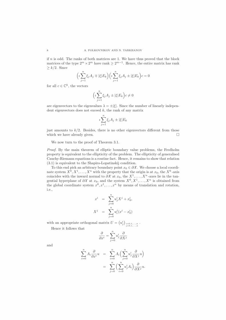
8 A. POLKOVNIKOV AND N. TARKHANOV
if n is odd. The ranks of both matrices are 1. We have thus proved that the blockmatrices of the type 2m×2m have rank ≥ 2m−1. Hence, the entire matrix has rank≥ k/2. Since (
ın∑
j=1
ξjAj ∓ |ξ|Ek
)(ı
n∑j=1
ξjAj ± |ξ|Ek
)c = 0
for all c ∈ Ck, the vectors
(ı
n∑j=1
ξjAj ± |ξ|Ek
)c �= 0
are eigenvectors to the eigenvalues λ = ±|ξ|. Since the number of linearly indepen-dent eigenvectors does not exceed k, the rank of any matrix
ın∑
j=1
ξjAj ± |ξ|Ek
just amounts to k/2. Besides, there is no other eigenvectors different from thosewhich we have already given. �
We now turn to the proof of Theorem 3.1.
Proof. By the main theorem of elliptic boundary value problems, the Fredholmproperty is equivalent to the ellipticity of the problem. The ellipticity of generalisedCauchy-Riemann equations is a routine fact. Hence, it remains to show that relation(3.1) is equivalent to the Shapiro-Lopatinskij condition.
To this end pick an arbitrary boundary point x0 ∈ ∂X . We choose a local coordi-nate system X0, X1, . . . , Xn with the property that the origin is at x0, the X
0 -axiscoincides with the inward normal to ∂X at x0, the X1, . . . , Xn -axes lie in the tan-gential hyperplane of ∂X at x0, and the system X0, X1, . . . , Xn is obtained fromthe global coordinate system x0, x1, . . . , xn by means of translation and rotation,i.e.,
xi =n∑
j=0
uijX
j + xi0,
Xj =n∑
j=0
uji (x
i − xi0)
with an appropriate orthogonal matrix U =(uij
)i=0,1,...,nj=0,1,...,n
.
Hence it follows that
∂
∂xi=
n∑j=0
uij
∂
∂Xj
andn∑
i=0
Ai∂
∂xiu =
n∑i=0
Ai
( n∑j=0
uij
∂
∂Xju)
=n∑
j=0
( n∑i=0
uijAi
) ∂
∂Xju.
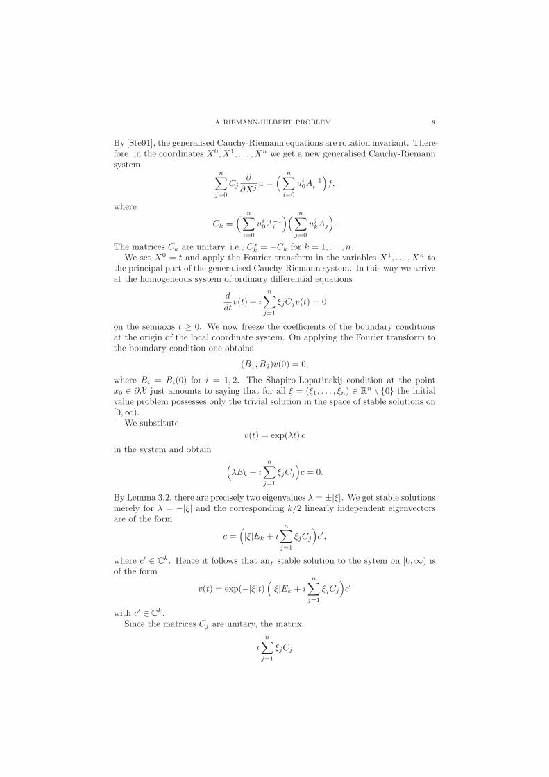
A RIEMANN-HILBERT PROBLEM 9
By [Ste91], the generalised Cauchy-Riemann equations are rotation invariant. There-fore, in the coordinates X0, X1, . . . , Xn we get a new generalised Cauchy-Riemannsystem
n∑j=0
Cj∂
∂Xju =
( n∑i=0
ui0A
−1i
)f,
where
Ck =( n∑
i=0
ui0A
−1i
)( n∑j=0
ujkAj
).
The matrices Ck are unitary, i.e., C∗k = −Ck for k = 1, . . . , n.
We set X0 = t and apply the Fourier transform in the variables X1, . . . , Xn tothe principal part of the generalised Cauchy-Riemann system. In this way we arriveat the homogeneous system of ordinary differential equations
d
dtv(t) + ı
n∑j=1
ξjCjv(t) = 0
on the semiaxis t ≥ 0. We now freeze the coefficients of the boundary conditionsat the origin of the local coordinate system. On applying the Fourier transform tothe boundary condition one obtains
(B1, B2)v(0) = 0,
where Bi = Bi(0) for i = 1, 2. The Shapiro-Lopatinskij condition at the pointx0 ∈ ∂X just amounts to saying that for all ξ = (ξ1, . . . , ξn) ∈ R
n \ {0} the initialvalue problem possesses only the trivial solution in the space of stable solutions on[0,∞).
We substitute
v(t) = exp(λt) c
in the system and obtain
(λEk + ı
n∑j=1
ξjCj
)c = 0.
By Lemma 3.2, there are precisely two eigenvalues λ = ±|ξ|. We get stable solutionsmerely for λ = −|ξ| and the corresponding k/2 linearly independent eigenvectorsare of the form
c =(|ξ|Ek + ı
n∑j=1
ξjCj
)c′,
where c′ ∈ Ck. Hence it follows that any stable solution to the sytem on [0,∞) is
of the form
v(t) = exp(−|ξ|t)(|ξ|Ek + ı
n∑j=1
ξjCj
)c′
with c′ ∈ Ck.
Since the matrices Cj are unitary, the matrix
ın∑
j=1
ξjCj
10 A. POLKOVNIKOV AND N. TARKHANOV
is Hermitean. Therefore, it can be reduced by means of a unitary matrix T to adiagonal form, T depending on ξ and U = (ui
j). We thus conclude that
ı
n∑j=1
ξjCj = |ξ|T(
Ek/2 00 −Ek/2
)T ∗
whence
v(t) = exp(−|ξ|t)(|ξ|Ek + |ξ|T
( Ek/2 00 −Ek/2
)T ∗
)c′
= 2|ξ| exp(−|ξ|t)T( Ek/2 0
0 0
)T ∗ c′.
Write
T =(
T 11 T 1
2
T 21 T 2
2
),
where T ij are (k/2× k/2) -matrices, and
T ∗c′ =(
zw
),
where z, w ∈ Ck/2. Then
v(t) = 2|ξ| exp(−|ξ|t)( T 1
1
T 21
)z
is a stable solution for arbitrary z ∈ Ck/2.
We substitute this formula into the initial value problem to obtain
(B1, B2) v(0) = |ξ| (B1, B2)( T 1
1
T 21
)z = 0.
Hence, v(t) = 0 if and only if z = 0. And the initial value problem possesses onlythe trivial solution if and only if
det
((B1, B2)
( T 11
T 21
))�= 0. (3.3)
We set
(Q1, Q2) := (B1, B2)T,
where Q1, Q2 are matrices of type k/2× k/2. Equality (3.3) means that
detQ1 �= 0.
Since detQ∗1 = detQ1, the relation detQ1 �= 0 is equivalent to detQ1Q
∗1 �= 0. Using
the equality
Q1Q∗1 +Q2Q
∗2 = Ek/2
A RIEMANN-HILBERT PROBLEM 11
we get
2Q1Q∗1 = (Q1, Q2)
(Ek/2 00 −Ek/2
)(Q∗
1
Q∗2
)+ Ek/2
= (B1, B2)T( Ek/2 0
0 −Ek/2
)T ∗
( B∗1
B∗2
)+ Ek/2
= (B1, B2)ı
|ξ|n∑
j=1
ξjCj
( B∗1
B∗2
)+ Ek/2
= ı((B1, B2)
n∑j=1
ξj|ξ|Cj
( B∗1
B∗2
)− ıEk/2
).
(3.4)
As already mentioned,
Ck =( n∑
i=0
ui0A
−1i
)( n∑j=0
ujkAj
)
whencen∑
k=1
ξk|ξ|Ck =
( n∑i=0
ui0A
−1i
)( ∑j=0,1,...,nk=1,...,n
ξk|ξ|u
jkAj
).
Obviously, the vector(ui0
)i=0,1,...,n
presents the inward normal vector ν and the
vector ( n∑j=1
ξj|ξ|u
ij
)i=0,1,...,n
is a tangential vector τ of length 1 at the boundary. Hence we get
n∑k=1
ξk|ξ| Ck =
( n∑i=0
νiA∗i
)( n∑j=0
τjAj
). (3.5)
On substituting this formula into (3.4) and taking into account that detQ1Q∗1 �= 0
we obtain
det (−2ıQ1Q∗1) = det
⎛⎝(B1, B2)
( n∑j=0
νjA∗j
)( n∑j=0
τjAj
)( B∗1
B∗2
)− ıEk/2
⎞⎠
�= 0,
as desired. �
Part 2. The Moisil-Teodoresco system
In this chapter we apply elliptic theory to a Riemann-Hilbert problem for theMoisil-Teodoresco system. For this purpose we construct an explicit Green for-mula which is of great importance to present the (formal) adjoint boundary valueproblem.
12 A. POLKOVNIKOV AND N. TARKHANOV
4. The Green formula
Consider the boundary value problem
Au :=
n∑j=0
Aj∂ju = f in X ,
Bu = u0 on ∂X ,
(4.1)
where we assume without restriction of generality that the matrices Aj are unitaryand B is a matrix of continuous functions on ∂X whose rank is maximal at eachpoint of the boundary.
Lemma 4.1. For all u, g ∈ C1(X ,Ck) it follows that∫∂X
g∗σ1(A)(ıν)u ds =
∫X(g∗Au− (A∗g)∗u) dx,
where ν is the inward unit normal vector for ∂X and ds the surface measure on theboundary ∂X .
As usual, A∗ stands for the formal adjoint of the differential operator A acting onfunctions with values in C
k. If one uses the canonical scalar product in Ck, then the
integrands of the boundary and spatial integrals can be written as (σ1(A)(ıν)u, g)xand (Au, g)x − (u,A∗g)x, respectively, where the sub x points out the pointwisescalar product of function values.
Proof. Using the Gauß formula yields∫∂X
g∗σ1(A)(ıν)u ds = −n∑
j=0
∫∂X
g∗Ajνju ds
=
∫X
n∑j=0
∂
∂xj(g∗Aju) dx
=
∫X
( n∑j=0
( ∂g
∂xj
)∗Aju+
n∑j=0
g∗Aj∂u
∂xj
)dx
=
∫X
(− (A∗g)∗u+ g∗Au
)dx,
as desired. �
Let B(x) be an arbitrary (l×k) -matrix of continuous functions on the boundarywith the property that l ≤ k and the rank of B(x) is equal to l for all x ∈ ∂X Weset l0 = l, l1 = k and choose an (l2 × k) -matrix C(x) of continuous functions on∂X , such that
rank(
B(x)C(x)
)= k (4.2)
for all x ∈ ∂X . Hence it follows that the (k × k) -matrix
T (x) :=( B(x)
C(x)
)∗( B(x)C(x)
)= B(x)∗B(x) + C(x)∗C(x)
is invertible and the entries of the inverse matrix T−1(x) are continuous functionson the boundary. Actually, the matrix C(x) can be chosen in such a way thatC(x)B(x)∗ = 0 for all x ∈ ∂X . This can be clarified within the framework of

A RIEMANN-HILBERT PROBLEM 13
compatibility complexes for sufficiently regular differential operators. To wit, westart with C0 = B∗.
Lemma 4.2. Suppose that C0(x) is an (l1× l0) -matrix of continuous functions onthe boundary whose rank is l0 for all x ∈ ∂X . Then there are (li+1 × li) -matricesCi(x) of continuous functions on the boundary, with i = 1, . . . , N −1, such that thesequence
0 −→ Cl0 C0(x)−→ C
l1 C1(x)−→ . . .CN−1(x)−→ C
lN −→ 0
is exact for each x ∈ ∂X .
Proof. We focus on the construction of the matrix C1(x) which is used in the sequel.To this end, we start with any matrix C(x) satisfying (4.2), and modify it in sucha way that C(x)B(x)∗ = 0 for all x ∈ ∂X . This latter condition just amounts tosaying that C(x) vanishes on the range of B(x)∗. For each fixed x ∈ ∂X , the spaceC
k decomposes into the orthogonal sum of the null space of B(x) and the range ofB(x)∗. Hence, we shall have got the desired modification of C(x) if we composeC(x) with the projection P (x) of Ck onto the null space of B(x). What is left isto show that there is any projection P (x) which depends continuously on x ∈ ∂X .Since the matrix B(x) has rank l, it follows that the (l × l) -matrix B(x)B(x)∗ isinvertible for all x ∈ ∂X and the entries of the inverse are continuous functions onthe boundary. Define
P (x) = Ek −B(x)∗(B(x)B(x)∗)−1B(x)
for x ∈ ∂X . Obviously, P (x) is the identity operator on the null space of B(x)and B(x)P (x) = B(x) − B(x) = 0, i.e., P (x) is a projection onto the null spaceof B(x) indeed. On the other hand, P (x) vanishes on the range of B(x)∗, forP (x)B(x)∗ = B(x)∗ − B(x)∗ = 0. Hence, on substituting C(x)P (x) for C(x) weobtain an (l2 × k) -matrix C1(x) with desired properties. �
We can thus choose C(x) = C1(x) to obtain CB∗ = 0 in (4.2). Note that T (x)just amounts to the Laplacian of the complex at step C
l1 . No attempt has beenmade here to develop the theory for pseudodifferential operators B on the boundary∂X .
Theorem 4.3. For all u, g ∈ C1(X ,Ck) it follows that∫∂X
((Cadjg)∗Bu− (Badjg)∗Cu
)ds =
∫X(g∗Au− (A∗g)∗u) dx,
whereCadj = BT−1(σ1(A)(ıν))∗,Badj = −CT−1(σ1(A)(ıν))∗. (4.3)
Proof. By the above, T−1(x)T (x) = Ek for all x ∈ ∂X . On substituting the formulafor T (x) one obtains(
T−1(x)B(x)∗)B(x) +
(T−1(x)C(x)∗
)C(x) = Ek.
We now substitute this decomposition into the formula of Lemma 4.1. Then theboundary integral reduces to∫
∂Xg∗σ1(A)(ıν)Ekuds =
∫∂X
g∗σ1(A)(ıν)((T−1B∗)Bu+
(T−1C∗)Cu
)ds
=
∫∂X
((Cadjg)∗Bu− (Badjg)∗Cu
)ds,
14 A. POLKOVNIKOV AND N. TARKHANOV
showing the theorem. �
The formula of Theorem 4.3 is called the Green formula for the boundary valueproblem {A,B} in the domain X . It allows one to introduce an adjoint boundaryvalue problem for {A,B}, this is given by {A∗, Badj}. A condition for the existenceof an elliptic adjoint boundary value problem is that the matrix B(x) can be sup-plemented with a matrix C(x) to a continuously invertible matrix on the boundaryof X . This is not always the case. Moreover, the adjoint boundary value prob-lem is not uniquely determined, for the supplement C(x) can be chosen in diversefashions.
Theorem 4.3 yields immediately a necessary condition for the existence of asolution u ∈ H1(X ,Ck) to problem (4.1) with given f and u0. We call it a solvabilitycondition of problem (4.1) for short.
Corollary 4.4. If problem (4.1) possesses a solution u ∈ H1(X ,Ck) in X then thedata f and u0 should satisfy∫
∂X(u0, C
adjg)xds =
∫X(f, g)xdx (4.4)
for all g ∈ H1(X ,Ck) such that A∗g = 0 in X and Badjg = 0 on ∂X .
Proof. We first observe that Theorem 4.3 holds not only for smooth functions u andg with values in C
k on the closure of X but also for all u, g ∈ H1(X ,Ck). To seethis it suffices to approximate the functions u and g of Sobolev class by functionsuj and gj which are C∞ in the closure of X . On writing the Green formula for uj
and gj and passing to the limit when j → ∞ we get the Green formula forfunctionsu and g of Sobolev class H1(X ,Ck). Equality (4.4) readily follows from the Greenformula. �
Corollary 4.4 initiates immediately a boundary value problem for solutions ofthe adjoint system A∗g = v in X . To wit,
A∗g := −n∑
j=0
A∗j∂jg = v in X ,
Badjg = g0 on ∂X ,
(4.5)
where Badj = −CT−1(σ1(A)(ıν))∗. Problem (4.5) is called the adjoint boundaryvalue problem for (4.1) with respect to the Green formula. We mention two extremecases of Corollary 4.4. If (l = k and) B(x) is invertible for all x ∈ ∂X , then (4.1) is aCauchy problem with data on the whole boundary. From CB∗ = 0 we deduce thatC = 0. Thus, the boundary operator Badj is zero and the adjoint problem (4.5)reduces to the inhomogeneous equation A∗g = v in X . Since A∗ is a generalisedCauchy-Riemann operator, the equation A∗g = v has a solution g ∈ H1(X ,Ck) forall data v ∈ L2(X ,Ck), the space of solutions being of infinite dimension. Condition(4.4) is known to be not only necessary but also sufficient for the solvability of theCauchy problem (4.1), see [Tar95, 10.1.3]. If (l = 0 then) the matrix B(x) is zero forall x ∈ ∂X , then problem (4.1) reduces to the inhomogeneous equation Au = f in X .Once again it has a solution u ∈ H1(X ,Ck) for all data f ∈ L2(X ,Ck) while the nullspace of A is infinite dimensional. By (4.2), the matrix C(x) should bear rank k ateach boundary point x. Hence, the adjoint (4.5) is a Cauchy problem for solutions ofA∗g = 0 in X with data on the entire boundary. This problem is normally solvable
A RIEMANN-HILBERT PROBLEM 15
and possesses at most one solution, see [Tar95, 10.1.3]. Formally, the conditionof Corollary 4.4 is necessary and sufficient for the solvability of (4.1). One mayconjecture that (4.4) is a necessary and sufficient condition for the solvability of(4.1) each time when this problem is Fredholm. But we have not been able toprove this.
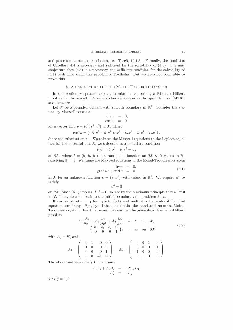
5. A calculation for the Moisil-Teodoresco system
In this section we present explicit calculations concerning a Riemann-Hilbertproblem for the so-called Moisil-Teodoresco system in the space R
3, see [MT31]and elsewhere.
Let X be a bounded domain with smooth boundary in R3. Consider the sta-
tionary Maxwell equationsdiv v = 0,curl v = 0
for a vector field v = (v1, v2, v3) in X , where
curlu =(−∂2v
2 + ∂1v3, ∂2v
1 − ∂0v3,−∂1v
1 + ∂0v2).
Since the substitution v = ∇p reduces the Maxwell equations to the Laplace equa-tion for the potential p in X , we subject v to a boundary condition
b0v1 + b1v
2 + b2v3 = u0
on ∂X , where b = (b0, b1, b2) is a continuous function on ∂X with values in R3
satisfying |b| = 1. We frame the Maxwell equations in the Moisil-Teodoresco system
div v = 0,gradu4 + curl v = 0
(5.1)
in X for an unknown function u = (v, u4) with values in R4. We require u4 to
satisfyu4 = 0
on ∂X . Since (5.1) implies Δu4 = 0, we see by the maximum principle that u4 ≡ 0in X . Thus, we come back to the initial boundary value problem for v.
If one substitutes −u4 for u4 into (5.1) and multiplies the scalar differentialequation containing −∂0u4 by −1 then one obtains the standard form of the Moisil-Teodoresco system. For this reason we consider the generalised Riemann-Hilbertproblem
A0∂u
∂x0+A1
∂u
∂x1+A2
∂u
∂x2= f in X ,(
b0 b1 b2 00 0 0 1
)u = u0 on ∂X
(5.2)
with A0 = E4 and
A1 =
⎛⎜⎜⎝
0 1 0 0−1 0 0 00 0 0 10 0 −1 0
⎞⎟⎟⎠ , A2 =
⎛⎜⎜⎝
0 0 1 00 0 0 −1
−1 0 0 00 1 0 0
⎞⎟⎟⎠ .
The above matrices satisfy the relations
AiAj +AjAi = −2δij E4,A∗
j = −Aj
for i, j = 1, 2.
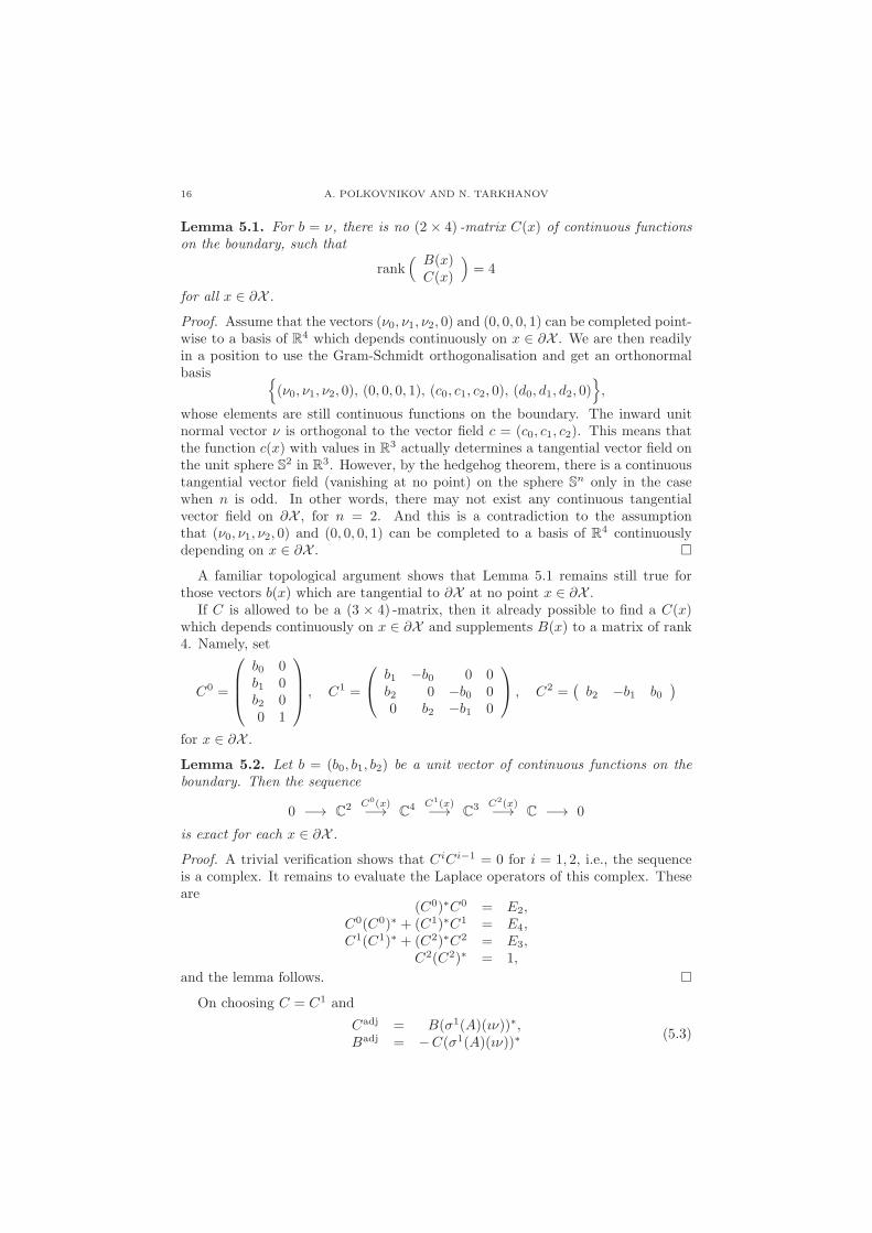
16 A. POLKOVNIKOV AND N. TARKHANOV
Lemma 5.1. For b = ν, there is no (2 × 4) -matrix C(x) of continuous functionson the boundary, such that
rank( B(x)
C(x)
)= 4
for all x ∈ ∂X .
Proof. Assume that the vectors (ν0, ν1, ν2, 0) and (0, 0, 0, 1) can be completed point-wise to a basis of R4 which depends continuously on x ∈ ∂X . We are then readilyin a position to use the Gram-Schmidt orthogonalisation and get an orthonormalbasis {
(ν0, ν1, ν2, 0), (0, 0, 0, 1), (c0, c1, c2, 0), (d0, d1, d2, 0)},
whose elements are still continuous functions on the boundary. The inward unitnormal vector ν is orthogonal to the vector field c = (c0, c1, c2). This means thatthe function c(x) with values in R
3 actually determines a tangential vector field onthe unit sphere S2 in R
3. However, by the hedgehog theorem, there is a continuoustangential vector field (vanishing at no point) on the sphere S
n only in the casewhen n is odd. In other words, there may not exist any continuous tangentialvector field on ∂X , for n = 2. And this is a contradiction to the assumptionthat (ν0, ν1, ν2, 0) and (0, 0, 0, 1) can be completed to a basis of R4 continuouslydepending on x ∈ ∂X . �
A familiar topological argument shows that Lemma 5.1 remains still true forthose vectors b(x) which are tangential to ∂X at no point x ∈ ∂X .
If C is allowed to be a (3 × 4) -matrix, then it already possible to find a C(x)which depends continuously on x ∈ ∂X and supplements B(x) to a matrix of rank4. Namely, set
C0 =
⎛⎜⎜⎝
b0 0b1 0b2 00 1
⎞⎟⎟⎠ , C1 =
⎛⎝ b1 −b0 0 0
b2 0 −b0 00 b2 −b1 0
⎞⎠ , C2 =
(b2 −b1 b0
)
for x ∈ ∂X .
Lemma 5.2. Let b = (b0, b1, b2) be a unit vector of continuous functions on theboundary. Then the sequence
0 −→ C2 C0(x)−→ C
4 C1(x)−→ C3 C2(x)−→ C −→ 0
is exact for each x ∈ ∂X .
Proof. A trivial verification shows that CiCi−1 = 0 for i = 1, 2, i.e., the sequenceis a complex. It remains to evaluate the Laplace operators of this complex. Theseare
(C0)∗C0 = E2,C0(C0)∗ + (C1)∗C1 = E4,C1(C1)∗ + (C2)∗C2 = E3,
C2(C2)∗ = 1,
and the lemma follows. �On choosing C = C1 and
Cadj = B(σ1(A)(ıν))∗,Badj = −C(σ1(A)(ıν))∗ (5.3)
A RIEMANN-HILBERT PROBLEM 17
we thus obtain the Green formula of Theorem 4.3 related to the Riemann-Hilbertproblem (5.2).
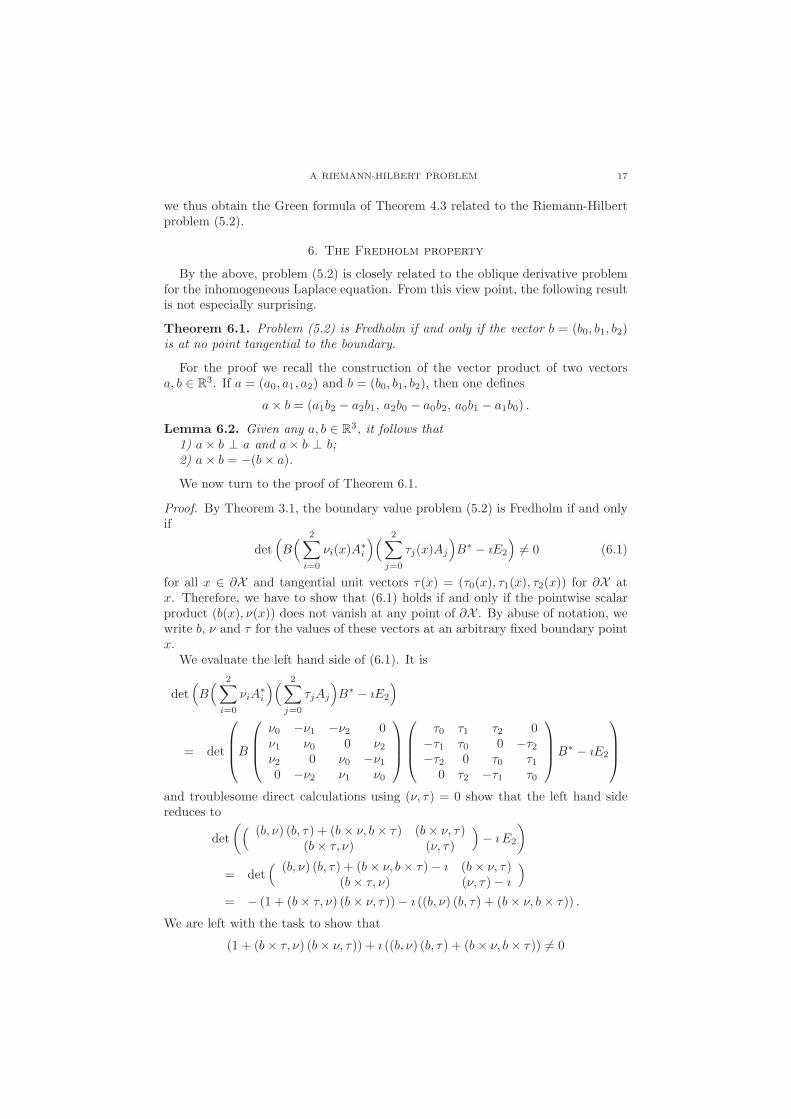
6. The Fredholm property
By the above, problem (5.2) is closely related to the oblique derivative problemfor the inhomogeneous Laplace equation. From this view point, the following resultis not especially surprising.
Theorem 6.1. Problem (5.2) is Fredholm if and only if the vector b = (b0, b1, b2)is at no point tangential to the boundary.
For the proof we recall the construction of the vector product of two vectorsa, b ∈ R
3. If a = (a0, a1, a2) and b = (b0, b1, b2), then one defines
a× b = (a1b2 − a2b1, a2b0 − a0b2, a0b1 − a1b0) .
Lemma 6.2. Given any a, b ∈ R3, it follows that
1) a× b ⊥ a and a× b ⊥ b;2) a× b = −(b× a).
We now turn to the proof of Theorem 6.1.
Proof. By Theorem 3.1, the boundary value problem (5.2) is Fredholm if and onlyif
det(B( 2∑
i=0
νi(x)A∗i
)( 2∑j=0
τj(x)Aj
)B∗ − ıE2
)�= 0 (6.1)
for all x ∈ ∂X and tangential unit vectors τ(x) = (τ0(x), τ1(x), τ2(x)) for ∂X atx. Therefore, we have to show that (6.1) holds if and only if the pointwise scalarproduct (b(x), ν(x)) does not vanish at any point of ∂X . By abuse of notation, wewrite b, ν and τ for the values of these vectors at an arbitrary fixed boundary pointx.
We evaluate the left hand side of (6.1). It is
det(B( 2∑
i=0
νiA∗i
)( 2∑j=0
τjAj
)B∗ − ıE2
)
= det
⎛⎜⎜⎝B
⎛⎜⎜⎝
ν0 −ν1 −ν2 0ν1 ν0 0 ν2ν2 0 ν0 −ν10 −ν2 ν1 ν0
⎞⎟⎟⎠
⎛⎜⎜⎝
τ0 τ1 τ2 0−τ1 τ0 0 −τ2−τ2 0 τ0 τ1
0 τ2 −τ1 τ0
⎞⎟⎟⎠B∗ − ıE2
⎞⎟⎟⎠
and troublesome direct calculations using (ν, τ) = 0 show that the left hand sidereduces to
det
(((b, ν) (b, τ) + (b× ν, b× τ) (b× ν, τ)
(b× τ, ν) (ν, τ)
)− ı E2
)
= det( (b, ν) (b, τ) + (b× ν, b× τ)− ı (b× ν, τ)
(b× τ, ν) (ν, τ)− ı
)= − (1 + (b× τ, ν) (b× ν, τ))− ı ((b, ν) (b, τ) + (b× ν, b× τ)) .
We are left with the task to show that
(1 + (b× τ, ν) (b× ν, τ)) + ı ((b, ν) (b, τ) + (b× ν, b× τ)) �= 0
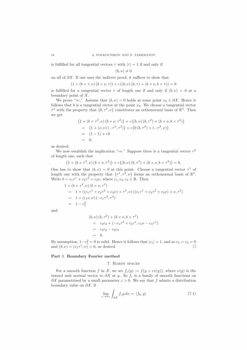
18 A. POLKOVNIKOV AND N. TARKHANOV
is fulfilled for all tangential vectors τ with |τ | = 1 if and only if
(b, ν) �= 0
on all of ∂X . If one uses the indirect proof, it suffices to show that
(1 + (b× τ, ν) (b× ν, τ)) + ı ((b, ν) (b, τ) + (b× ν, b× τ)) = 0
is fulfilled for a tangential vector τ of length one if and only if (b, ν) = 0 at aboundary point of X .
We prove “⇐.” Assume that (b, ν) = 0 holds at some point x0 ∈ ∂X . Hence itfollows that b is a tangential vector at the point x0. We choose a tangential vectorτ2 with the property that {b, τ2, ν} constitutes an orthonormal basis of R3. Thenwe get (
1 + (b× τ2, ν) (b× ν, τ2))+ ı
((b, ν) (b, τ2) + (b× ν, b× τ2)
)=
(1 + (ν, ν) (−τ2, τ2)
)+ ı
(0 (b, τ2) + (−τ2, ν)
)= (1− 1) + ı 0
= 0,
as desired.We now establish the implication “⇒.” Suppose there is a tangential vector τ2
of length one, such that(1 + (b× τ2, ν) (b× ν, τ2)
)+ ı
((b, ν) (b, τ2) + (b× ν, b× τ2)
)= 0.
One has to show that (b, ν) = 0 at this point. Choose a tangential vector τ1 oflength one with the property that {τ1, τ2, ν} forms an orthonormal basis of R3.Write b = c1τ
1 + c2τ2 + c3ν, where c1, c2, c3 ∈ R. Then
1 + (b× τ2, ν) (b× ν, τ2)
= 1 + ((c1τ1 + c2τ
2 + c3ν)× τ2, ν) ((c1τ1 + c2τ
2 + c3ν)× ν, τ2)
= 1 + (c1ν, ν) (−c1τ2, τ2)
= 1− c21
and
(b, ν) (b, τ2) + (b× ν, b× τ2)
= c3c2 + (−c1τ2 + c2τ
1, c1ν − c3τ1)
= c3c2 − c2c3
= 0.
By assumption, 1−c21 = 0 is valid. Hence it follows that |c1| = 1, and so c2 = c3 = 0and (b, ν) = (c1τ
1, ν) = 0, as desired. �
Part 3. Boundary Fourier method
7. Hardy spaces
For a smooth function f in X , we set fε(y) := f(y + εν(y)), where ν(y) is theinward unit normal vector to ∂X at y. So fε is a family of smooth functions on∂X parametrised by a small parameter ε > 0. We say that f admits a distributionboundary value on ∂X , if
limε→0+
∫∂X
fεg ds =: 〈f0, g〉 (7.1)
A RIEMANN-HILBERT PROBLEM 19
exists for all g ∈ C∞comp(∂X ). In this case the limit defines a distribution f0 on the
boundary and the convergence is not only in the weak sense but also in the strongtopology on D′(∂X ).
The local structure of harmonic functions admitting distribution boundary valuesis well known.
Theorem 7.1. For a harmonic function f in X , the following properties are equiv-alent:
1) f admits a distribution boundary value on ∂X .2) f is in the Sobolev space H−s(X ), for some integer s.3) There exist an integer N and C > 0, such that |f(x)| ≤ C/(dist(x, ∂X ))N for
all x ∈ X .4) For any x0 ∈ ∂X there are a neighbourhood U in R
n and a function h har-monic in U ∩X and continuous in U ∩X , such that f = 〈c, ∂〉Nh in U ∩X , wherec ∈ R
n is a constant vector and N an integer.
Proof. See [Str84, Theorem 1.1]. The proof actually shows that, for a harmonicfunction f which admits a distribution boundary value on ∂X , this boundary valueis the trace of f on ∂X in the sense of Sobolev spaces, i.e., f0 ∈ H−s−1/2(∂X )provided f ∈ H−s(X ). �
From Theorem 7.1 it follows that if f is a harmonic function in X which admitsa distribution boundary value on ∂X then∑
|α|≤m
bα(x) ∂αf
also admits a distribution boundary value on ∂X whenever the coefficients bα areC∞ in the closure of X . It is worth pointing out that this function need not beharmonic.
Just as in the case of more familiar harmonic Hardy spaces, the Poisson inte-gral mediates between boundary values and the corresponding harmonic functions.Given a distribution f0 on ∂X , we write P (f0) for the Poisson integral of f0. It isdefined by P (f0)(x) = 〈P (x, ·), f0〉 for x ∈ X , where P (x, y) is the Poisson kernelfor X , i.e., the normal derivative of the Green function G(x, y) at y ∈ ∂X . For eachinteger s, the Poisson integral induces an isomorphism of H−s−1/2(∂X ) onto thesubspace of H−s(X ) consisting of harmonic functions in X . Its inverse is the mapassigning to each harmonic function f ∈ H−s(X ) its boundary value, see Corollary1.7 in [Str84].
Yet another designation for functions in X , which are polynomially bounded in1/dist(x, ∂X ), is functions of finite order of growth near the boundary, cf. Chapter 9in [Tar95] and elsewhere. By the above, a harmonic function of finite order of growthnear the boundary in X is uniquely determined by its distribution boundary valueon ∂X . This allows one to identify harmonic functions of finite order of growthin X with their boundary values on ∂X . In this way we obtain many interestingBanach spaces of harmonic functions in the domain X . The most popular of themis perhaps the Hardy space H2(X ). This space is defined to consist of all harmonicfunctions in X of finite order of growth near the boundary, whose distributionboundary values on ∂X belong to L2(∂X ). When endowed with L2(∂X ) -norm,H2(X ) is a Hilbert space.
20 A. POLKOVNIKOV AND N. TARKHANOV
Let now u be a smooth function in X with values in Ck satisfying a generalised
Cauchy-Riemann system Au = 0 in X . If there exist an integer N and C > 0,such that |u(x)| ≤ C/(dist(x, ∂X ))N for all x ∈ X , then the same is true for thecomponents of u. By Theorem 7.1, each component admits a distribution boundaryvalue on ∂X . Hence, u admits a boundary value on ∂X which is a continuous linearfunctional on C∞
comp(∂X ,Ck). Moreover, both Bu and Cu admit boundary values
on ∂X which are distributions with values in Ck. This is precisely the sense in
which we interpret them in the following formula analogous to the Cauchy integralformula.
Let e(x) be the standard fundamental solution of convolution type for Δ, i.e.,e(x) = (2π)−1 log |x|, if n = 2, and
e(x) =1
σn
1
2− n
1
|x|n−2,
if n ≥ 3, where σn is the surface area of the unit sphere in Rn. The matrix Φ = −A∗e
is a (two-sided) fundamental solution of convolution type of the operator A, i.e., thefundamental equations ΦA = AΦ = I hold on compactly supported distributionsin R
n with values in Ck.
Lemma 7.2. For each solution u to equations Au = 0 in X of finite order of growthnear ∂X , it follows that
−∫∂X
((Bu,CadjΦ(x− ·)∗)y − (Cu,BadjΦ(x− ·)∗)y
)ds =
{ u(x), if x ∈ X ,0, if x ∈ R
n \ X .(7.2)
Note that (Φ(x − y))∗ = (Ae)(x − y) for all x and y away from the diagonal ofR
n, as is easy to check.
Proof. See Theorem 9.4.1 of [Tar95]. �This reasoning, when looked at from a more general point of view, leads to new
investigations of Fredholm boundary value problems in Hardy spaces, see [Tar95,11.2.2].
8. The Cauchy problem
For u ∈ H2(X )k, the Green formula (7.2) displays the Cauchy data of u on theboundary of X with respect to the operator A. These are weak limit values of Buand Cu on ∂X . Hence we formulate the Cauchy problem as follows: Given anyu0 ∈ L2(∂X ,Cl0) and u1 ∈ L2(∂X ,Cl2), find a function u ∈ H2(X )k satisfyingAu = 0 in X and {
Bu = u0,Cu = u1
(8.1)
on ∂X . In order that there may exist a solution u ∈ H2(X )k to problem (8.1),it is necessary that there be a function u ∈ L2(∂X ,Ck) satisfying Bu = u0 andCu = u1.
Lemma 8.1. Suppose u0 ∈ L2(∂X ,Cl0) and u1 ∈ L2(∂X ,Cl2). For the existenceof a function u ∈ L2(∂X ,Ck) satisfying Bu = u0 and Cu = u1 it is necessary andsufficient that
BT−1(B∗u0 + C∗u1) = u0,CT−1(B∗u0 + C∗u1) = u1.
(8.2)
A RIEMANN-HILBERT PROBLEM 21
Proof. Necessity. From the equalities Bu = u0 and Cu = u1 on the boundary itfollows that u = T−1(B∗u0 + C∗u1). On substituting this formula into Bu = u0
and Cu = u1 we obtain (8.2).Sufficiency. Set u = T−1(B∗u0+C∗u1). Then u ∈ L2(∂X ,Ck) satisfies Bu = u0
and Cu = u1, which is due to (8.2). �
The Cauchy problem for solutions of systems with injective symbol and data onthe whole boundary was intensively studied in the 1960s. To a certain extent thisstudy was motivated by the paper [Cal63]. The study of the Cauchy problem inHardy spaces is motivated by the problem of analytic continuation, cf. Chapter 11in [Tar95].
Theorem 8.2. Let u0 ∈ L2(∂X ,Cl0) and u1 ∈ L2(∂X ,Cl2). In order that theremay be a solution u ∈ H2(X )k to Au = 0 in X subject to (8.1), it is necessary andsufficient that (u0, u1) would satisfy (8.2) and∫
∂X
((u0, C
adjg)x − (u1, Badjg)x
)ds = 0 (8.3)
for all g ∈ SA∗(X ).
Proof. Necessity. If u ∈ H2(X )k is a solution of the Cauchy problem with data u0,u1, then u0 = Bu and u1 = Cu satisfy (8.2), which is due to Lemma 8.1. Moreover,by the Green formula,∫
∂X
((u0, C
adjg)x − (u1, Badjg)x
)ds =
∫∂X
((Bu,Cadjg)x − (Cu,Badjg)x
)ds
= 0
for all g ∈ SA∗(X ), as required.Sufficiency. We introduce a function U in X \ ∂X with values in C
k by theGreen-type integral
U(x) = −∫∂X
((u0, C
adjΦ(x− ·)∗)y − (u1, BadjΦ(x− ·)∗)y
)ds, (8.4)
where x ∈ X \ ∂X . An easy calculation using (5.3) shows that
(u0, CadjΦ(x− ·)∗)y − (u1, B
adjΦ(x− ·)∗)y = Φ(x− ·)(σ1(A)(ıν)ub)
on ∂X , where
ub = T−1 (B∗u0 + C∗u1) .
By (8.2), we get Bub = u0 and Cub = u1, and so ub is of class L2(∂X ,Ck) ifand only if u0 and u1 belong to L2(∂X ,Cl0) and L2(∂X ,Cl2), respectively. Thus,formula (8.4) reduces to
U = −Φ ∗ ([∂X ]σ1(A)(ıν)ub)
in X \ ∂X .For each fixed x ∈ X \X , the columns of the matrix Φ(x−·)∗ belong to SA∗(X ).
Hence, (8.3) implies that U vanishes in the complement of X .Set u = U �X . We next prove that u is the desired solution of the Cauchy
problem. This is equivalent to saying that u ∈ H2(X )k and Au = 0 in X , u �∂X= ub
at ∂X .From the structure of the fundamental matrix Φ it follows immediately that u
belongs to H2(X )k and satisfies Au = 0 in X . Since ub ∈ L2(∂X ,Ck), the jump of
22 A. POLKOVNIKOV AND N. TARKHANOV
the double layer potential Φ([∂X ]σub) under crossing the surface ∂X from X \X toX just amounts to ub. This is true even for all distributions ub on ∂X taking theirvalues in C
k, see Theorem 10.1.5 in [Tar95]. For the square integrable densities ub
the jump is understood in an appropriate sense including the L2(∂X ,Ck) -norm.Summarising we conclude that u �∂X= ub, for U vanishes in X \X . This completesthe proof. �
9. Operator-theoretic foundations
The operator-theoretic foundations of the method of Fischer-Riesz equationsare elaborated in [Tar95, 11.1]. It goes back at least as far as [PF50]. Here weadapt this method for studying the Hilbert boundary value problem for generalisedCauchy-Riemann equations.
Any solution of generalised Cauchy-Riemann equations in X is a k -column ofharmonic functions in this domain. Therefore, the k -fold product of the Hardyspace
H2(X )k = H2(X )× . . .×H2(X )︸ ︷︷ ︸k times
fits well to constitute the domain of problem (4.1), where f = 0. More precisely,denote by H1 the vector space of all u ∈ H2(X )k satisfying Au = 0 in X . Whenendowed with the L2(∂X ,Ck) -norm, this space is complete, i.e., a Hilbert space.The operator B maps H1 continuously into H2 = L2(∂X ,Cl0), it need not beone-to-one or onto.
LetH be the subspace of L2(∂X ,Cl0)×L2(∂X ,Cl2) consisting of all pairs (u0, u1)satisfying (8.2). Obviously, this subspace is closed, and so it is a Hilbert spaceunder the unitary structure induced from the Cartesian product. According toLemma 8.1, the space H just amounts to the image of L2(∂X ,Ck) by the mappingu �→ (Bu,Cu).
Lemma 9.1. As defined above, the space H coincides with the Cartesian productH2 × imC, where imC stands for the range of C : L2(∂X ,Ck) → L2(∂X ,Cl2).
Proof. From what has already been said it follows thatH is a subspace ofH2×imC.Hence, we shall have established the lemma if we prove that both H2 × {0} and{0} × imC belong to H.
Pick an arbitrary u0 ∈ L2(∂X ,Cl0). Since the Laplacian T 0 = BB∗ at step 0 ofthe the compatibility complex of Lemma 4.2 is invertible at each point of ∂X , weget u0 = Bu, where u = B∗(T 0)−1u0 belongs to L2(∂X ,Ck). From the equalityCB∗ = 0 we see that Cu = 0, and so the pair (u0, 0) = (Bu,Cu) belongs to H, asdesired.
Consider now a pair (0, u1), where u1 = Cu for some u ∈ L2(∂X ,Ck). Withoutloss of generality we can assume that Bu = 0 on the boundary, for if not, we replaceu by C∗(T 2)−1u1, where T
2 = (C2)∗C2+C1(C1)∗ is the Laplacian at step 2 of thecompatibility complex of Lemma 4.2. Then (0, u1) = (Bu,Cu) belongs to H, andso {0} × imC lies in H. �
Recall that the image of L2(∂X ,Ck) by C = C1 coincides with the kernel of C2
in L2(∂X ,Cl2), which is a consequence of Lemma 4.2. Therefore, the range of Cis a closed subspace of L2(∂X ,Cl2), and so a Hilbert space with induced unitarystructure.
A RIEMANN-HILBERT PROBLEM 23
Consider the mappingM : H1 → H given byMu = (Bu,Cu), which correspondsto the Cauchy problem for solutions of Au = 0 in X with Cauchy data Bu = u0
and Cu = u1 on ∂X . By the above, M is continuous. From Theorem 8.2 it followsthat M has closed range.
Denote by M∗ : H → H1 the operator that is adjoint to M : H1 → H in thesense of Hilbert spaces.
Lemma 9.2. The null-space imM∗ of the operator M∗ is separable in the topologyinduced from H.
Proof. This is true by the school fact that any subspace of a separable metric spaceis separable. �
Let SA∗(X ) stand for the space of all solutions to the formal adjoint systemA∗g = 0 on neighbourhoods of X . Since A∗ is elliptic, these are real analyticfunctions with values in C
k.
Lemma 9.3. Assume that g ∈ SA∗(X ). Then the couple (Cadjg,−Badjg) belongsto imM∗.
Proof. Using formulas (5.3) we see that the operator Badj factors through C, towit, Badj = −CT−1(σ1(A)(ıν))∗. Hence it follows that the couple (Cadjg,−Badjg)belongs to H.
It remains to prove that (Mu, (Cadjg,−Badjg))H = 0 for all u ∈ H1. By theGreen formula, we get
(Mu, (Cadjg,−Badjg))H =
∫∂X
((Bu,Cadjg)x − (Cu,Badjg)x
)ds
= 0,
as desired. �
The subspace of imM∗ consisting of all elements of the form (Cadjg,−Badjg),where g ∈ SA∗(X ), is separable. Hence, there are many ways to choose a sequence{gi}i=1,2,... in SA∗(X ), such that the system {(Cadjgi,−Badjgi)} is complete in thissubspace.
In Example 9.6 we will show some explicit sequences {gi} with this property.For the moment we fix one of such sequences.
Lemma 9.4. As defined above, the system {(Cadjgi,−Badjgi)}i=1,2,... is completein imM∗.
Proof. Let F be a continuous linear functional on imM∗ vanishing on each elementof the system {(Cadjgi,−Badjgi)}. Since imM∗ is a closed subspace of H, the Rieszrepresentation theorem implies the existence of an element (u0, u1) ∈ imM∗, suchthat the action of F on imM∗ consists in scalar multiplication with the element(u0, u1). In particular,
F(Cadjgi,−Badjgi) =
∫∂X
((Cadjgi, u0)x − (Badjgi, u1)x
)ds
= 0
for all i = 1, 2, . . .. Since the system {(Cadjgi,−Badjgi)}i=1,2,... is dense in thesubspace of imM∗ consisting of all elements of the form (Cadjg,−Badjg), where
24 A. POLKOVNIKOV AND N. TARKHANOV
g ∈ SA∗(X ), we get ∫∂X
((u0, C
adjg)x − (u1, Badjg)x
)ds = 0
for all g ∈ SA∗(X ). We now use Theorem 8.2 which says that there exists a functionu ∈ H2(X )k such that Au = 0 in X and Bu = u0, Cu = u1 at the boundary ofX . In other words, (u0, u1) = Mu. Hence it follows that F(h) = (h,Mu)H = 0for all h ∈ imM∗. Thus, F ≡ 0 and the standard application of the Hahn-Banachtheorem completes the proof. �
Write P for the projection of H = H2 × imC onto the first factor. The compo-sition PM = B acting from H1 to H2 just amounts to the operator of boundaryvalue problem (4.1) with f = 0 in the updated setting. More precisely, given anyu0 ∈ L2(∂X ,Cl0), find u ∈ H2(X )k satisfying Au = 0 in X and Bu = u0 weakly onthe boundary of X . The following lemma expresses the most important propertyof the system {gi}.Lemma 9.5. The system {Badjgi}i=1,2,... is complete in the image of L2(∂X ,Ck)by C if and only if PM is injective.
Proof. By the Hahn-Banach theorem, {Badjgi} is complete in the image imC ofL2(∂X ,Ck) by C if and only if any continuous linear functional F on imC vanishingon each element of the system, is zero. Pick such a functional F . By the Rieszrepresentation theorem there is a function u1 ∈ imC such that F(h) = (h, u1) forall h ∈ imC. Using Lemma 9.1 we see that (0, u1) belongs to the space H. So weget
((0, u1), (Cadjgi,−Badjgi))H = −(Badjgi, u1)L2(∂X ,Cl2 )
= −F(Badjgi)
= F(CT−1(σ1(A)(ıν))∗gi)= 0
for all i = 1, 2, . . .. On applying Lemma 9.4 we deduce that the element (0, u1)belongs to the orthogonal complement of the subspace imM∗ in H. Since theoperator M has closed range, the orthogonal complement of imM∗ coincides withthe range of M . Hence, there is a function u ∈ H2(X )k satisfying Au = 0 in Xand Bu = 0, Cu = u1 on ∂X . If the operator PM is injective, then u = 0 whenceu1 = 0 and F = 0. Conversely, if the functional F is different from zero, then u1 isnot zero and so the operator PM fails to be injective, which is precisely the desiredconclusion. �
After removing the elements which are linear combinations of the previous onesfrom the system {Badjgi}i=1,2,..., we get a sequence {gin} in SA∗(X ), such thatthe system {Badjgin} is linearly independent. Applying then the Gram-Schmidtorthogonalisation to the system {Badjgin} in L2(∂X ,Cl2), we obtain a new system{en}n=1,2,... in SA∗(X ), such that {Badjen} is an orthonormal system in L2(∂X ,Cl2).Moreover, {Badjen} is an orthonormal basis in the image of L2(∂X ,Ck) by C, pro-vided that PM is injective. Note that the elements en of the new system haveexplicit expressions through the elements {gi1 , . . . , gin} of the old system in theform of Gram’s determinants.
A RIEMANN-HILBERT PROBLEM 25
Example 9.6. Since X is a bounded domain with smooth boundary, its comple-ment has only finitely many connected components. Let {xi} be a finite set ofpoints in R
n \ X , such that each connected component of Rn \ X contains at leastone point xi. Then the columns of the matrix ∂αΦ(xi − ·)∗ belong to SA∗(X ) andthe system {Badj∂αΦ(xi−·)∗} is complete in the subspace of L2(X ,Cl2) formed byelements of the type Badjg with g ∈ SA∗(X ).
The proof of this fact actually repeats the reasoning of Example 11.4.14 in[Tar95]. Apparently the system of Example 9.6 is most convenient for numericalsimulations.
Part 4. Application to the Riemann-Hilbert problem
10. The Fischer-Riesz equations
Let {gi}i=1,2,... be an arbitrary sequence in SA∗(X ) with the property that thesystem {(Cadjgi,−Badjgi)} is complete in imM∗. Applying the Gram-Schmidtorthogonalisation to the system {Badjgi} in L2(∂X ,Cl2), we obtain a new system{en}n=1,2,... in SA∗(X ), such that the system {Badjen} is orthonormal in the spaceL2(∂X ,Cl2).
Given any u1 ∈ L2(∂X ,Cl2), we denote by kn(u1) the Fourier coefficients of u1
with respect to the system {Badjen}, i.e.,
kn(u1) =
∫∂X
(u1, Badjen)y ds
for n = 1, 2, . . ..
Lemma 10.1. If u ∈ H2(∂X )k satisfies Au = 0 in X , then
kn(Cu) =
∫∂X
(Bu,Cadjen)y ds,
where n = 1, 2, . . ..
Proof. Using Lemma 9.3 we obtain
kn(Cu) =
∫∂X
(Cu,Badjen)y ds+ (Mu, (Cadjen,−Badjen))H
=
∫∂X
(Bu,Cadjen)y ds,
as desired. �
Thus, in order to find the Fourier coefficients of the data Cu on the boundarywith respect to the system {Badjen} in L2(∂X ,Cl2), it suffices to know only thedata Bu of problem (4.1).
Theorem 10.2. Let u0 ∈ L2(∂X ,Cl0). In order that there be a u ∈ H2(X )k suchthat Au = 0 in X and Bu = u0 on ∂X , it is necessary and sufficient that
1)∞∑
n=1
|cn|2 < ∞, where cn =
∫∂X
(u0, Cadjen)y ds, and
2)
∫∂X
(u0, Cadjg)y ds = 0 for all g ∈ SA∗(X ) satisfying Badjg = 0 on the bound-
ary.
26 A. POLKOVNIKOV AND N. TARKHANOV
Proof. Necessity. Suppose there is a function u ∈ H2(X )k satisfying Au = 0 in Xand Bu = u0 at ∂X . Then cn = kn(Cu) for all n = 1, 2, . . ., which is due to Lemma10.1. Applying the Bessel inequality yields
∞∑n=1
|cn|2 =∞∑
n=1
|kn(Cu)|2 ≤∫∂X
|Cu|2 ds < ∞,
and 1) is proved. On the other hand, 2) follows immediately from the Greenformula.
Sufficiency. We now assume that 1) and 2) are satisfied. Condition 1) implies,by the Fischer-Riesz theorem, that the series
u1 =∞∑
n=1
cnBadjen (10.1)
converges in the space L2(∂X ,Cl2). Since the summands of series (10.1) belongto the image of L2(∂X ,Ck) by C and the range of C is closed, it follows thatu1 ∈ imC. Hence, the pair (u0, u1) actually belongs to H. Obviously, {cn}n=1,2,...
are the Fourier coefficients of u1 with respect to the orthonormal system {Badjen}in L2(∂X ,Cl2). In other words, we get cn = kn(u1) for all n = 1, 2, . . .. On substi-tuting formulas for cn from 1) into these equalities we arrive at the orthogonalityrelations ∫
∂X
((u0, C
adjen)y − (u1, Badjen)y
)ds = 0 (10.2)
for n = 1, 2, . . ., cf. (8.3).Our next goal is to prove that the pair (u0, u1) is actually orthogonal to all
elements of the system {(Cadjgi,−Badjgi)}i=1,2,... in H, this latter being completein imM∗. To do this, let us recall how the system {en} has been obtained fromthe system {gi}.
Even if the system {(Cadjgi,−Badjgi)} is linearly independent in H, the system{Badjgi} may have elements which are linear combinations of the previous onesin the space L2(∂X ,Cl2). Such elements should be eliminated from the systembefore applying the Gram-Schmidt orthogonalisation. For example, suppose that,for some i, the equality
Badjgi =i−1∑j=1
ci,j Badjgj
is fulfilled with suitable complex numbers ci,j . Consider the function
g′i = gi −i−1∑j=1
ci,j gj
which belongs to SA∗(X ). Obviously, (Cadjg′i,−Badjg′i) lies in imM∗ and satisfiesBadjg′i = 0. It follows that
gi =i−1∑j=1
ci,j gj + g′i.
All the other elements (Cadjgi,−Badjgi), except for the eliminated ones, are ex-pressed, by the contents of Gram-Schmidt orthogonalisation, as linear combina-tions of the elements {(Cadjen,−Badjen)}n=1,...,i. Thus, any element of the system
A RIEMANN-HILBERT PROBLEM 27
{(Cadjgi,−Badjgi)} has a unique expression through the elements of the system{(Cadjen,−Badjen)}n=1,2,... in the form
gi =
i∑n=1
ci,n en + g′i, (10.3)
where g′i ∈ SA∗(X ) satisfies Badjg′i = 0 on the boundary ∂X .From equalities (10.2) and (10.3) and condition 2) of the theorem it follows
immediately that
((u0, u1), (Cadjgi,−Badjgi))H
=
i∑n=1
ci,n ((u0, u1), (Cadjen,−Badjen))H + ((u0, u1), (C
adjg′i,−Badjg′i))H
= 0
for all i = 1, 2, . . .. Since the system {(Cadjgi,−Badjgi)}i=1,2,... is complete inimM∗, the element (u0, u1) belongs to the orthogonal complement of this subspacein H. Using the lemma of operator kernel annihilator, we deduce that there existsa function u ∈ H1 satisfying Mu = (u0, u1). In particular, u ∈ H2(X )k satisfiesAu = 0 in X and Bu = u0 on ∂X , i.e., u is the desired solution of boundary valueproblem (4.1). �
The convergence of the series in 1) guarantees the stability of boundary valueproblem (4.1). Under this condition, the range of the mapping PM is described interms of continuous linear functionals on the space H, cf. 2) , which is impossiblein the general case.
Corollary 10.3. Under the hypotheses of Theorem 10.2, if moreover the homoge-neous adjoint boundary value problem (4.5) has no smooth solutions in X differentfrom zero, then for problem (4.1) to possess a solution u ∈ H2(X )k it is necessaryand sufficient that
∞∑n=1
|cn|2 < ∞.
Proof. This follows immediately from Theorem 10.2 since condition 2) is automat-ically fulfilled. �
11. Regularisation of solutions
Note that the proof of Theorem 10.2 works without the assumption that theoperator PM in H is injective. Our next objective will be to construct an approx-imate solution to the boundary value problem of (4.1) with f = 0. To this end itis natural to assume that the corresponding homogeneous boundary value problemhas only zero solution in the space H2(X )k, i.e., the mapping PM is injective. Inthis case the orthonormal system {Badjen} is actually complete in the image ofL2(∂X ,Ck) by C. The orthonormal bases of this form are said to be special, cf.[Tar95, 11.3].
For x ∈ X \∂X , we denote by kn(BadjΦ(x−·)∗) the k -row whose entries are the
Fourier coefficients of the columns of the (l2×k) -matrix BadjΦ(x−·)∗ with respect
28 A. POLKOVNIKOV AND N. TARKHANOV
to the orthonormal basis {Badjen}n=1,2,... in the image of L2(∂X ,Ck) by C. Moreprecisely, we set
kn(BadjΦ(x− ·)∗) =
∫∂X
(BadjΦ(x− ·)∗, Badjen)y ds
for n = 1, 2, . . ..
Lemma 11.1. For n = 1, 2, . . ., the coefficients kn(BadjΦ(x − ·)∗) are analytic
functions in X \ ∂X with values in (Ck)∗.
Proof. The assertion is obvious, for the fundamental solution Φ(x − y) is analyticaway from the diagonal of X × X . �
Consider the following (Schwartz) kernels RN defined for x ∈ X \ ∂X and y in aneighbourhood of X :
RN (x, y) = Φ(x− y)−N∑
n=1
kn(BadjΦ(x− ·)∗)∗ en(y)∗,
where N = 1, 2, . . ..
Lemma 11.2. As defined above, the kernels RN are analytic in x ∈ X \∂X and y ina neighbourhood of X except for the diagonal {x = y}, and A∗(y,D)RN (·− y)∗ = 0on this set.
Proof. This follows immediately from Lemma 11.1 and the fact that en ∈ SA∗(X ),as desired. �
The sequence {RN} provides a very special approximation of the fundamentalsolution Φ.
Lemma 11.3. The sequence {BadjRN (x, ·)∗}N=1,2,... converges to zero in the normof L2(∂X ,Cl2×k) uniformly in x on compact subsets of X \ ∂X .
Proof. In fact, we get
BadjRN (x, ·)∗ = BadjΦ(x− ·)∗ −N∑
n=1
Badjen kn(BadjΦ(x− ·)∗)
=
∞∑n=N+1
Badjen kn(BadjΦ(x− ·)∗)
for each fixed x ∈ X \ ∂X . The right-hand side of this equality is a remainderof the Fourier series of the element BadjRN (x, ·)∗ with respect to the orthonormalbasis {Badjen} in the image of L2(∂X ,Ck) by C. Hence, it tends to zero in theL2(∂X ,Cl2×k) -norm, as N → ∞. This proves the first part of the lemma. Thesecond part follows from a general remark on Fourier series, for the mapping ofX \ ∂X to L2(∂X ,Cl2×k) given by
x �→ BadjΦ(x− ·)∗is continuous. �
The convergence of the approximations allows one to reconstruct solutions u ofthe class H2(X ,Ck) to Au = 0 in X through their data Bu.
A RIEMANN-HILBERT PROBLEM 29
Theorem 11.4. Every function u ∈ H2(X )k satisfying Au = 0 in X can be repre-sented by the integral formula
u(x) = limN→∞
(−
∫∂X
(Bu,CadjRN (x, ·)∗)y ds)
for all x ∈ X .
Proof. Fix a point x ∈ X . Since RN (x, ·)∗ and Φ(x−·)∗ differ by a k -row of smoothsolutions of the system A∗g = 0 in a neighbourhood of X , one can write by theGreen formula
u(x) = −∫∂X
((Bu,CadjRN (x, ·)∗)y − (Cu,BadjRN (x, ·)∗)y
)ds (11.1)
for any N = 1, 2, . . .. From u ∈ H2(X )k we deduce that Cu ∈ L2(∂X ,Cl2). Henceit follows by Lemma 11.3 that
limN→∞
∫∂X
(Cu,BadjRN (x, ·)∗)y ds = 0.
Thus, letting N → ∞ in (11.1) establishes the formula. �As mentioned, for many problems of mathematical physics formulas for approxi-
mate solution like that of Theorem 11.4 were earlier obtained by Kupradze and hiscolleagues, see [Kup67].
12. Solvability of elliptic boundary value problems
We can now return to the Sobolev space setting of boundary value problem (4.1)which is H1 = H1(X ,Ck). Given any u ∈ H1(X ,Ck), both Au and Bu are welldefined in L2(X ,Ck) and H1/2(∂X ,Cl0), respectively. Hence, the analysis doesnot require any function spaces of negative smoothness. More generally, let s be anatural number. Given any u0 in Hs−1/2(∂X ,Cl0), we look for a u ∈ Hs(X ,Ck)satisfying (4.1). Theorem 10.2 still applies to establish the existence of a weaksolution u ∈ H2(X )k, provided that the conditions 1) and 2) are fulfilled. To inferthe existence of a Sobolev space solution, one needs a regularity theorem for weaksolutions in H2(X )k saying that any weak solution belongs actually to the Sobolevspace Hs(X ,Ck). This is the case if (4.1) is an elliptic boundary value problem,i.e., the pair {A,B} satisfies the Shapiro-Lopatinskij condition on the boundary ofX .
Corollary 12.1. Suppose a regularity theorem holds for boundary value problem(4.1). Let u0 ∈ Hs−1/2(∂X ,Cl0), where s = 1, 2, . . .. Then, in order that there bea u ∈ Hs(X ,Ck) satisfying Au = 0 in X and Bu = u0 on ∂X it is necessary andsufficient that
1)
∞∑n=1
|cn|2 < ∞, where cn =
∫∂X
(u0, Cadjen)y ds, and
2)
∫∂X
(u0, Cadjg)y ds = 0 for all g ∈ SA∗(X ) satisfying Badjg = 0 at the bound-
ary.
Proof. It is sufficient to prove the sufficiency of conditions 1) and 2) . If the con-ditions 1) and 2) are satisfied, then there exists a function u ∈ H2(X )k, suchthat Au = 0 in X and Bu = u0 on ∂X . For solutions of Au = 0 in X thecondition u ∈ H2(X )k just amounts to saying that u ∈ H1/2(X ,Ck). Since
30 A. POLKOVNIKOV AND N. TARKHANOV
Au ∈ Hs−1(X ,Ck) and Bu ∈ Hs−1/2(∂X ,Cl0), the regularity theorem impliesthat u ∈ Hs(X ,Ck), as desired. �
Assume that both the problem {A,B} and its adjoint {A∗, Badj} with respect tothe Green formula are elliptic. This is the case only if l0 = l2, and so their commonvalue amounts to k/2. By the Fredholm property, the space of all g ∈ SA∗(X )satisfying Badjg = 0 on ∂X , is finite dimensional. Moreover, the condition 2) aloneis sufficient for the existence of a solution u ∈ Hs(X ,Ck) to problem (4.1). Hence itfollows that for elliptic boundary value problems the condition 1) is automaticallyfulfilled.
Thus, the regularity problem for weak solutions of (4.1) is still of primary char-acter in the study of boundary value problems. On the other hand, our approachdemonstrates rather strikingly that Theorem 11.4 is of great importance for numer-ical simulation.
Acknowledgements The first author gratefully acknowledges the financial sup-port of the DAAD (Deutscher Akademischer Austauschdienst) und the RussianMinistry of Education, No 1.719.2016/2.2, and the grant of the Russian FederationGovernment for scientific research under the supervision of leading scientist at theSiberian Federal University, contract No 14.Y26.31.0006.
A RIEMANN-HILBERT PROBLEM 31
References
[Agr97] Agranovich, M. S., Elliptic Boundary Value Problems, In: Encyclopaedia of Mathe-matical Sciences, Vol. 79, Springer, Berlin et al., 1997, 1–144.
[AT13] Alsaedy, A., and Tarkhanov, N., The method of Fischer-Riesz equations for elliptic
boundary value problems, J. of Complex Analysis 1 (2013), Issue 1, 1–11.
[AT16] Alsaedy, A., and Tarkhanov, N., A Hilbert boundary value problem for generalised
Cauchy-Riemann equations, Advances in Applied Clifford Algebras 27 (2017), Issue
2, 931–953.
[Cal63] Calderon, A. P., Boundary value problems for elliptic equations, In: “Outlines Joint
Symposium PDE” (Novosibisrk, 1963), Acad. Sci. USSR, Siberian Branch, Moscow,
1963, 303–304.
[Gak77] Gakhov, F. D., Boundary Value Problems, Nauka, Moscow, 1977.
[Kup67] Kupradze, V. D., Approximate solution of problems of mathematical physics, UspekhiMat. Nauk 22 (1967), No. 2, 59–107.
[MT31] Moisil, G. C., and Teodorescu, N., Fonction holomorphic dans l’espace, Bul. Soc. St.
Cluj 6 (1931), 177–194.[PF50] Picone, M., and Fichera, G., Neue funktional-analytische Grundlagen fur die Exis-
tenzprobleme und Losungsmethoden von Systemen linearer partieller Differentialgle-
ichungen, Monatsh. Math. 54 (1950), 188–209.
[Ste91] Stern, I., Boundary value problems for generalized Cauchy-Riemann systems in the
space, In: “Boundary value and initial value problems in complex analysis: Studies
in complex analysis and its applications to partial differential equations, I” (Halle,
1988), Pitman Res. Notes Math. Ser., Vol. 256, Longman Sci. Tech., Harlow, 1991.
[Ste93a] Stern, I., On the existence of Fredholm boundary value problems for generalized
Cauchy-Riemann systems, Complex Variables 21 (1993), 19–38.
[Ste93b] Stern, I., Direct methods for generalized Cauchy-Riemann systems in the space, Com-
plex Variables 23 (1993), 73–100.
[Str84] Straube, E. J., Harmonic and analytic functions admitting a distribution boundary
value, Ann. Scuola Norm. Super. Pisa 11 (1984), No. 4, 559–591.
[Tar95] Tarkhanov, N., The Cauchy Problem for Solutions of Elliptic Equations, Akademie
Verlag, Berlin, 1995.
[Vol65] Volevich, L. R., On the solvability of boundary value problems for general elliptic
systems, Mat. Sb. 68 (110) (1965), No. 3, 373–416.
Siberian Federal University, Institute of Mathematics and Computer Science, pr.
Svobodnyi 79, 660041 Krasnoyarsk, Russia
E-mail address: [email protected]
Institute of Mathematics, University of Potsdam, Karl-Liebknecht-Str. 24/25, 14476
Potsdam, Germany
E-mail address: [email protected]