management v management accounting prof. dr. alfred luhmer winter 2006/07 fakultät für...
Post on 19-Dec-2015
213 views
TRANSCRIPT

Management VManagement Accounting
Prof. Dr. Alfred LuhmerWinter 2006/07
http://www.uni-magdeburg.de/bwl1/MACC/index.htm
Fakultät für Wirtschaftswissenschaft
OTTO-VON-GUERICKE-UNIVERSITÄT MAGDEBURG

2
Management V:Management Accounting
Textbook:
Charles T. Horngren, George Foster & Srikant M. Datar: Cost Accounting -
A Managerial Emphasis, 12th ed. 2006 (Prentice Hall)
see also:Robert S. Kaplan & Anthony A. Atkinson:
Advanced Management Accounting3rd ed. 1998 (Prentice Hall)

3
Supporting Devices
Text book: I expect that everybody has read the chapter
announced to be treated in each session (see „Announcement“ on the web site)
Web site: www.uni-magdeburg.de/bwl1/MACCcontains Slides additional exercises additional material

4
Contributions out of the audience during the lecture yield bonus points for the final exam
Rules:1. Participants can offer to present the solution to an exercise
immediately before the discussion takes place. No reservations in advance.
2. Solutions presented are weighted (in % of the exam), graded and recorded for each participant.
3. Any participant having presented a certain number of exercises is no longer eligible to give an additional presentation as long as anybody else with a lower number of presentations given offers a solution to the respective exercise. (Fairness rule)
4. Presentations worth x% of the exam reduce the weight of the written exam to (100 – x)%, presentations with grade below the grade of the exam are ignored; x cannot exceed 50.
5. Final exam must be passed (grade at least 4.0) for bonus points to have value.
5
Introduction
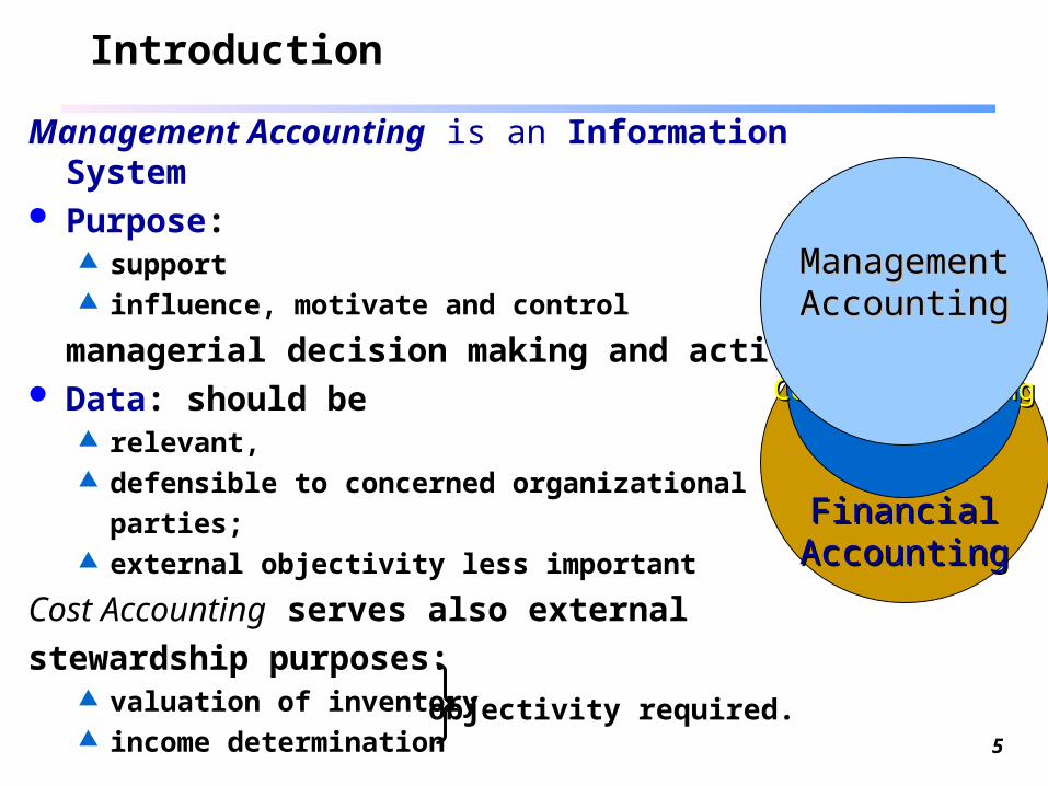
Management Accounting is an Information System Purpose:
support influence, motivate and control
managerial decision making and activity. Data: should be
relevant, defensible to concerned organizational
parties; external objectivity less important
Cost Accounting serves also external
stewardship purposes: valuation of inventory income determination
objectivity required.
FinancialFinancialAccountingAccounting
Cost AccountingCost Accounting
ManagementManagementAccountingAccounting
6
Historical PerspectiveManagerial Accounting originated from managed hierarchical enterprises
running large scale factories with multi-stage production
had to replace information provided formerly from market transactions between independent enterprises for
each stage of the production informal experience accumulation in a slowly changing
environment
long term investments require long term planning focus on internal cost efficiency
Suggested reading: H. Thomas Johnson & Robert S. Kaplan, Relevance Lost, The Rise and Fall of Management Accounting, Boston 1987 (Harvard Business School Press)

7
Early Pioneers of Management Accounting 19th century Railroads Steel producers: Andrew Carnegie
(born 1835 in Scotland. Emigrated 1848, died 1919*) developed a cost control system using
unit costs (per ton of rails) decomposed by cost categories
comparisons between periods and with competitors ratio measures to summarize information on cost
structureenabling him to calculate appropriate costs for nonstandard projects.
Merchandisers: Sears-Roebuck, Woolworth developed ratio systems to measure profitability and
turnover rate.
*) See: http://www.pbs.org/wgbh/amex/carnegie/sfeature/meet.html
Andrew Carnegie
8
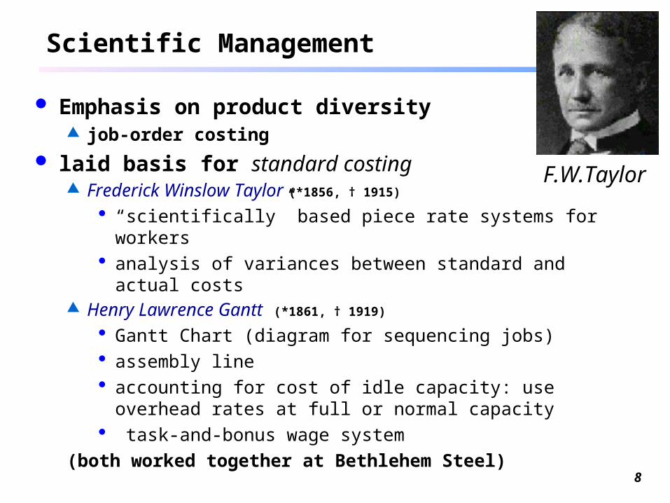
Scientific Management
Emphasis on product diversity job-order costing
laid basis for standard costing Frederick Winslow Taylor (*1856, † 1915)
“scientifically” based piece rate systems for workers analysis of variances between standard and actual costs
Henry Lawrence Gantt (*1861, † 1919)
Gantt Chart (diagram for sequencing jobs) assembly line accounting for cost of idle capacity: use overhead rates at full
or normal capacity task-and-bonus wage system
(both worked together at Bethlehem Steel)
F.W.Taylor
9
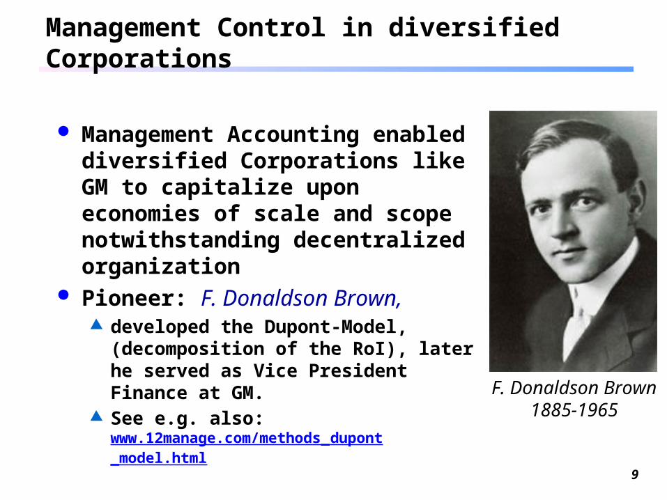
Management Control in diversified Corporations
Management Accounting enabled diversified Corporations like GM to capitalize upon economies of scale and scope notwithstanding decentralized organization
Pioneer: F. Donaldson Brown,
developed the Dupont-Model, (decomposition of the RoI), later
he served as Vice President Finance at GM.
See e.g. also: www.12manage.com/methods_dupont_model.html
F. Donaldson Brown1885-1965

10
Donaldson Brown (1885-1965) graduated from Virginia Polytechnic Institute in 1902, did graduate work in engineering at Cornell, and joined DuPont in 1909 as an explosives salesman. His financial acumen became apparent in 1912 when he submitted an efficiency report to the Executive Committee that utilized a return on investment formula. Treasurer John J. Raskob took Brown under his wing and encouraged him to develop uniform accounting procedures and other standard statistical formulas that enabled division managers to evaluate performance companywide despite the great diversification of the late 1910s. In 1918 Brown helped Raskob execute DuPont’s heavy investment in General Motors stock, and when he took over the treasurer’s office from Raskob the same year, he brought in economists and statisticians, an exceptional practice at the time. Brown joined the Executive Committee in 1920.By 1921 DuPont had gained a controlling interest in the flagging General Motors Corporation, and Pierre du Pont made Brown GM’s vice president of finance. Brown helped bring about GM’s financial recovery and in 1923 he developed the mechanisms that allowed DuPont to retain the GM investment. Brown was appointed to GM’s Executive Committee in 1924, and working with President Alfred P. Sloan, he refined the cost accounting techniques that he had been developing at DuPont. The principles of return on investment, return on equity, forecasting, and flexible budgeting were subsequently widely adopted in corporate America. Brown retired as an active executive of GM in 1946 but remained on the boards of both GM and DuPont. In 1959 he was one of four DuPont directors who resigned from GM’s board due to the Supreme Court’s 1959 antitrust decision.
(From http://Dupont.com)
11
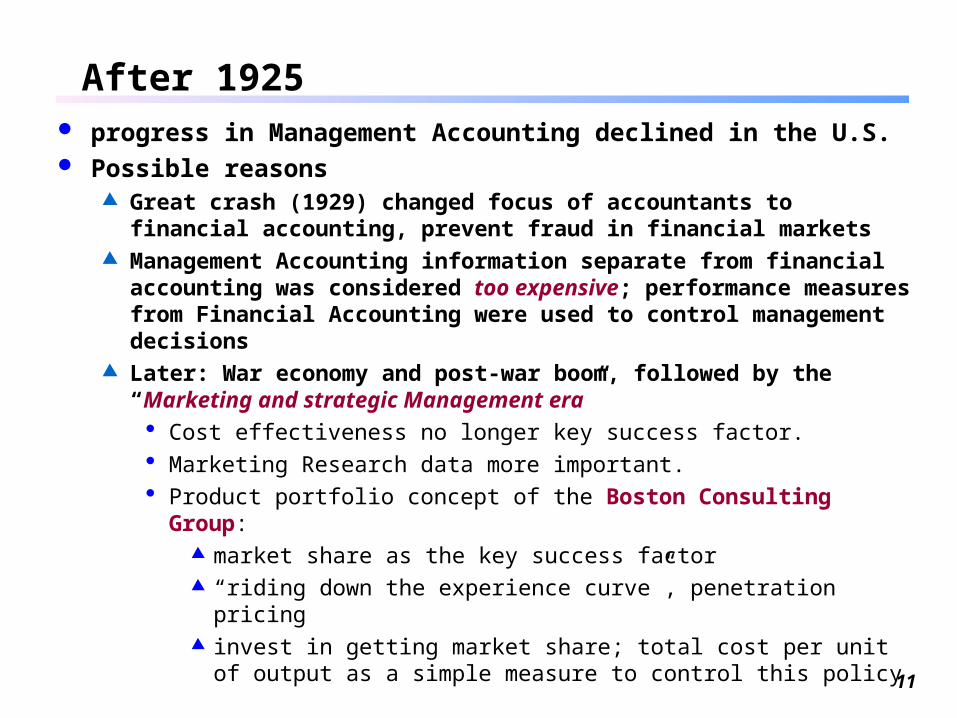
After 1925 progress in Management Accounting declined in the U.S. Possible reasons
Great crash (1929) changed focus of accountants to financial accounting, prevent fraud in financial markets
Management Accounting information separate from financial accounting was considered too expensive; performance measures from Financial Accounting were used to control management decisions
Later: War economy and post-war boom, followed by the “Marketing and strategic Management era”
Cost effectiveness no longer key success factor. Marketing Research data more important. Product portfolio concept of the Boston Consulting Group:
market share as the key success factor “riding down the experience curve”, penetration pricing invest in getting market share; total cost per unit of output as a
simple measure to control this policy

12
Developments in the 1980s
Competition from Japanese companies using continuous improvement of
processes design product quality
instead of “riding down the experience curve” reducing inventory because it inhibits improvement using CIM to reduce data acquisition cost trying to enhance response times to customer requests
1980s: Production regains attention: “Total Quality Management”
“Quality is free” production Management based on nonfinancial data such as
defectives in total production (ppm) yield rates, first-pass yields, rework and scrappage rates timely delivery rates turnover rates manufacturing cycle time

13
Later on
1990s: Systems point of view: IT influences: CIM
Data IntegrationMaterial Requirements Planning
Systems develop into Enterprise Resource Planning Systems and
Integrated Enterprise data bases with e-business portals (Internet and/or intranet-based e-Business workplaces, e.g. mySAP®)
Supply chain ManagementBalanced Scorecard

14
Financial performance measurement innovations introduced in the 1980s
Activity-based Costing and Management better tracing of resource costs to products,
services, and customers cost driver analysis ideas of standard costing are integrated (Activity-
based Budgeting)

15
Developments in Germany
Hierarchies of contribution margins to analyze product and program profitability (Pioneer: Paul Riebel *1918, †2001)
Refinement of standard costing Cost Driver Analysis for cost centers,
overlapping cost variances (Pioneer: Wolfgang Kilger *1927, † 1986)
Profit Planning based on multilinear models of operations
(pioneered by the OR group of Hoesch Steel Corp. at Dortmund, Gert Lassmann)
16
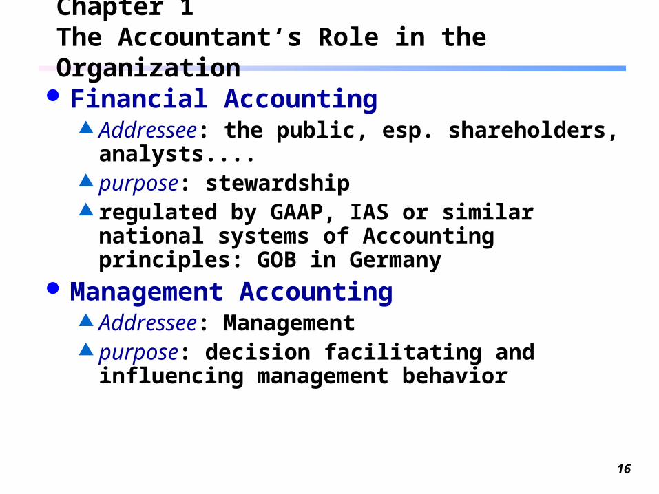
Chapter 1The Accountant‘s Role in the Organization
Financial Accounting Addressee: the public, esp. shareholders,
analysts.... purpose: stewardship regulated by GAAP, IAS or similar national
systems of Accounting principles: GOB in Germany
Management Accounting Addressee: Management purpose: decision facilitating and influencing
management behavior

17
Decision facilitating - using planning and control
Planning Strategic Planning: develops a vision of the business Long Range Planning: decides on programs and projects to implement
the strategy Budgeting: sets goals as standards to be achieved by projects or
responsibility centers in a defined period of time Basis for control coordinates plans and actions of different decision makers
Action choice: develops alternatives and selects actions for achieving budgeted goals
Control Action: implements an action Performance Evaluation: identifies deviations between actual and
planned performance Feedback: informs Planning on deviations as a basis for adaptation of
plans

18
Management Control Cycle(Robert N. Anthony: The Management Control Function, Boston, 1988, p.80 )
Budgeting
Evaluation
Pro
gram
min
gE
xecution
actionbu
dget
rev
isio
n
consideringnew strategies
19
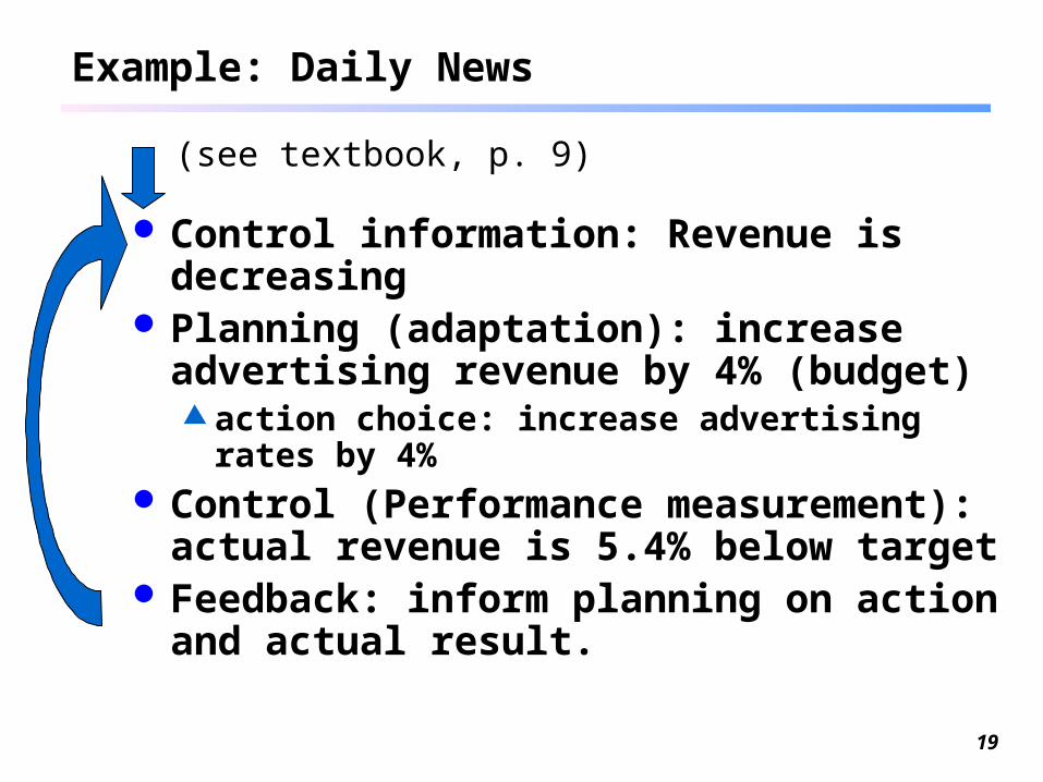
Example: Daily News
Control information: Revenue is decreasing
Planning (adaptation): increase advertising revenue by 4% (budget) action choice: increase advertising rates by
4% Control (Performance measurement):
actual revenue is 5.4% below target Feedback: inform planning on action and
actual result.
(see textbook, p. 9)

20
Performance Report
(see textbook, p.10)
Actual
(1)
Budget
(2)
(3) =
(1) – (2)
(4) =
(3)/(2)
Advertising pages sold
760 800 - 40
(U)
5%
Average rate per page
$5,080 $5,200 -$120 (U) 2.3%
Advertising revenues
$3,860T $4,160T -$299.2T (U)
7.2%

21
Example, economic analysis
Planning assumes (at least implicitly) a certain demand function, depending on price and selling effort + other influences
other things equal, an increase in price enhances revenue only if the slope of the price-demand function is nonnegative or if price is lower than at its revenue-maximizing level
(if marginal costs are positive then price should exceed marginal cost)
if none of these condition holds, then Naomi’s plan puts pressure on sales people: either shift the price-demand function upward
Shifting upward would require a change in the media quality or reduce the slope parameter
Usually they will only be able to reduce the slope parameter by approaching more people who might want to place an ad.

22
What happened? Sales people seem to have
tried to get sales by lowering prices instead of increasing approaches to customers
They increased the slope parameter only slightly
The revenue effect was perilous
of course: this argument rests on further assumptions... original slope = -0.1 linear demand function
Consequences: It seems harder than
assumed by Naomi to extend the demand potential
can one enhance media quality?
... ???
Naomi’s plan
Naomi’s plan
ex post
ex post
old actual
old actual
100
$1000

23
Roles of Accounting
Decision facilitating: support managers’ problem solving providing information information processing, analysis of ex post results suggest modeling approach
Scorekeeping: collecting and documenting data creating a common information base to limit quarreling esp. for performance measurement and responsibility
accounting
Attention directing: give hints to management on tasks to be completed consequences to consider
24
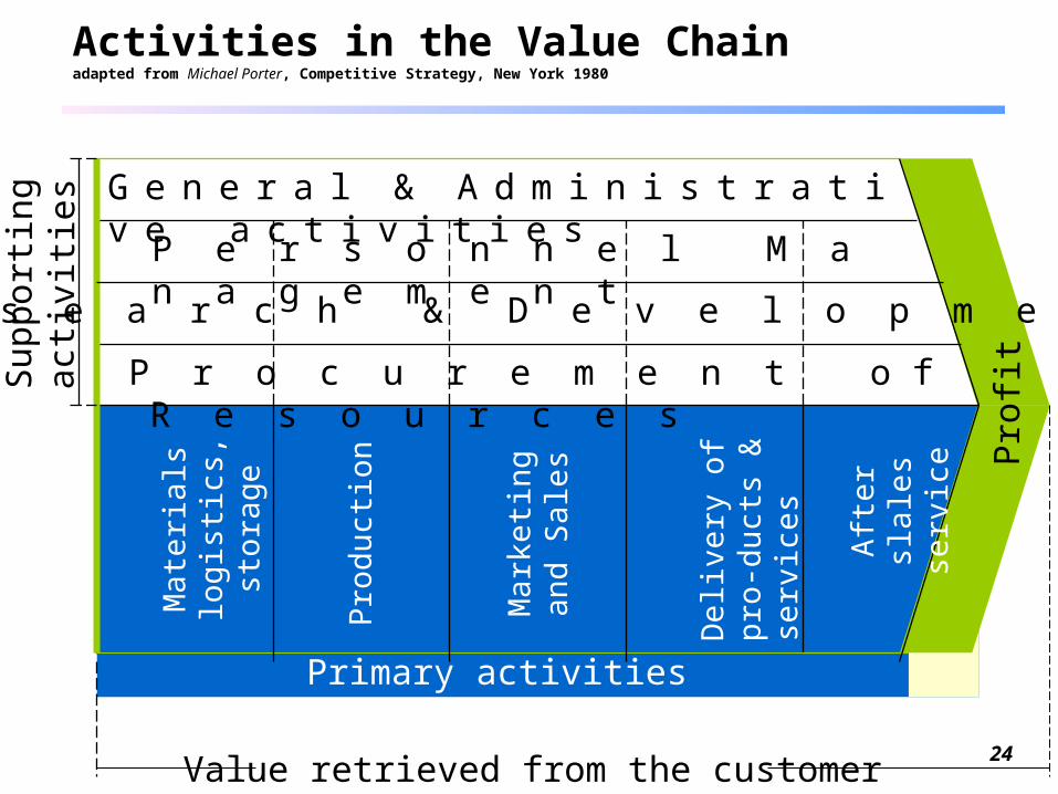
Activities in the Value Chainadapted from Michael Porter, Competitive Strategy, New York 1980
Ma t
e ri a
l s
log i
s tic
s ,s t
o ra g
e
De l
ive r
y o f
pr o
-d u
c ts
&
s er v
i ce s
Aft
er s
lale
s s e
r vi c
e
Ma r
k etin
g a n
d S
a le s
Pro
d uc t
i on
G e n e r a l & A d m i n i s t r a t i v e a c t i v i t i e s
P e r s o n n e l M a n a g e m e n t
P r o c u r e m e n t o f R e s o u r c e s
R e s e a r c h & D e v e l o p m e n t
Pro
fit
Primary activities
Sup
port
ing
activ
ities
Value retrieved from the customer

25
Focus of Management Accounting
Customer focus customer satisfaction customer profitability
Key success factors, e.g. Cost Quality Time Innovation
Continuous improvement of processes

26
Ethical Issues
Fundamental problem: ethical behavior and individual welfare
Methodological individualism: each individual is autonomous in defining aims and objectives to guide life
Actions of each individual have external effects on the welfare of others
Society needs rules and sanctions (“institutions”) to coordinate individual actions such that one individual seeking her welfare will not do too much harm to others
Law: formal institutions restricting allowed behavior• Sanctions: criminal justice, being sued before court
Morale: Tacit consent on restrictions to be honored by every one when aiming at enhancement of welfare
• sanctions: contempt, outcast• different sub-“societies” may have conflicting
morales

27
An example: Case B, p. 17
Bidder B offers all-expenses-paid weekend to the Super Bowl to management accountant A
Assumptions on valuations: A’s values:
participating without distorting analysis: 10 participating and biased analysis: 15
B’s values: Cost of weekend: 1 Bias in the accountant’s analysis: 10
Game matrix:
0
0
10
-1
0
0
15
9
A: no bias to analysis
positive bias in favor of B
B: no offer offer
28
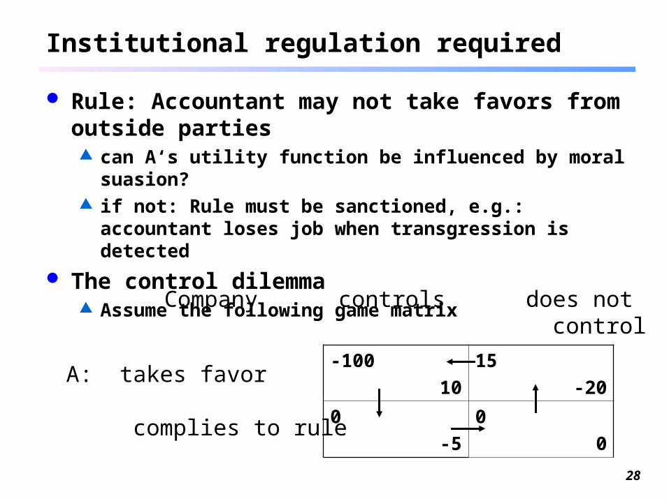
Institutional regulation required
Rule: Accountant may not take favors from outside parties can A‘s utility function be influenced by moral suasion? if not: Rule must be sanctioned, e.g.: accountant loses job
when transgression is detected
The control dilemma Assume the following game matrix
-100
10
15
-20
0
-5
0
0
A: takes favor
complies to rule
Company controls does not control
29
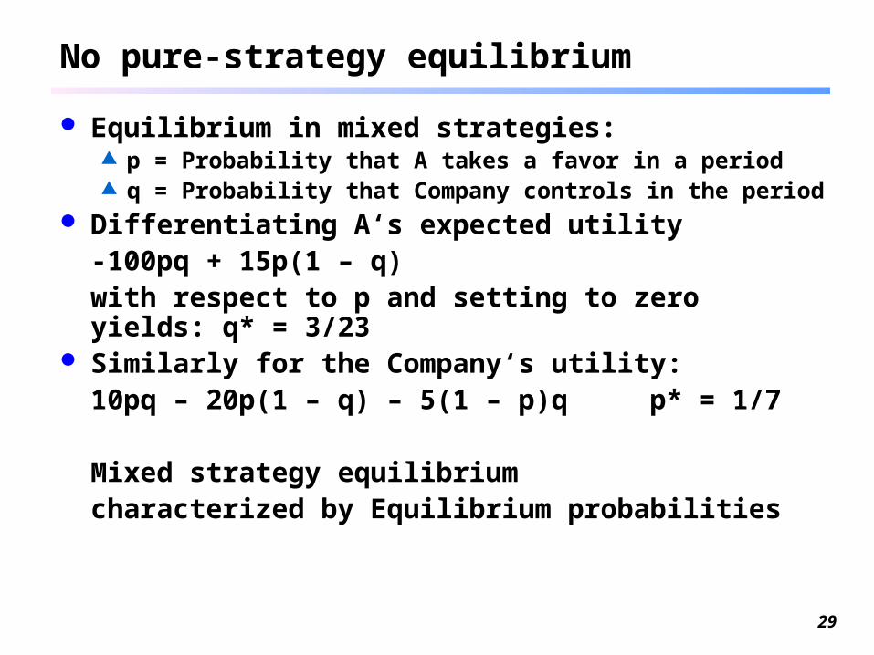
No pure-strategy equilibrium
Equilibrium in mixed strategies: p = Probability that A takes a favor in a period q = Probability that Company controls in the period
Differentiating A‘s expected utility-100pq + 15p(1 – q)with respect to p and setting to zero yields: q* = 3/23
Similarly for the Company‘s utility:10pq – 20p(1 – q) – 5(1 – p)q p* = 1/7
Mixed strategy equilibrium characterized by Equilibrium probabilities

30
CC Problems to be discussed
Problem 1-24, 1-25: Consider the decisions a. - d. and suggest how Management Accounting could have been involved in them. Propose detailed plans for economic analysis of what happened. (10%)
Problem 1-30: Additional information: Assume Cheng loses bonus payments if the proposal is not
accepted (valuation: -10) Shareholders lose money when the bribe is detected before
court (-10), they win 10, when it goes undetected and they get the contract
the state values the bribe being paid at –20 and incur control costs of 2, when control occurs.
Add a game theoretic analysis.
31
Chapter 2Cost Terms and Purposes
Cost and Cost Object
A cost is any resource sacrificed to achieve a specific objective.
The objective is called a cost object, e.g.
a product a service a customer a product category a period
a project R&D reorganization
an activity a department

32
Cost and Cost Objects, cont’d
Costs Cost objects
direct cost of A
direct cost of B
A
B
O
Assignment
Tracing
indirect costs Allocation
If B is an activityused exclusivelyby O then its cost can also be traced to O

33
Cost Behavior Patterns
Variable vs. Fixed variable costs: vary automatically with output
volume special cases:
proportional costs step cost functions: piecewise constant due to
indivisible input units
fixed costs: determined by past management decisions; can be changed only by new decisions special cases:
committed costs: cannot be changed at all during a specific commitment period
sunk costs: cannot be changed at all.

34
Cost drivers
Both fixed and variable costs depend not only on input prices but also on other influencing factors (cost drivers).
Example: Setup costs. variable with output volume, because larger volume will require
more setups but there is another intervening variable: lot size.
Setup costs per period = setup frequency cost per setup
Setup costs per period = price component
Lot size is subject to managerial decision. Cost drivers may be used to shape the dependence of variable cost
on output volume!
=volume/lot size
price component
1lot size
cost driverscost drivers
volume
35
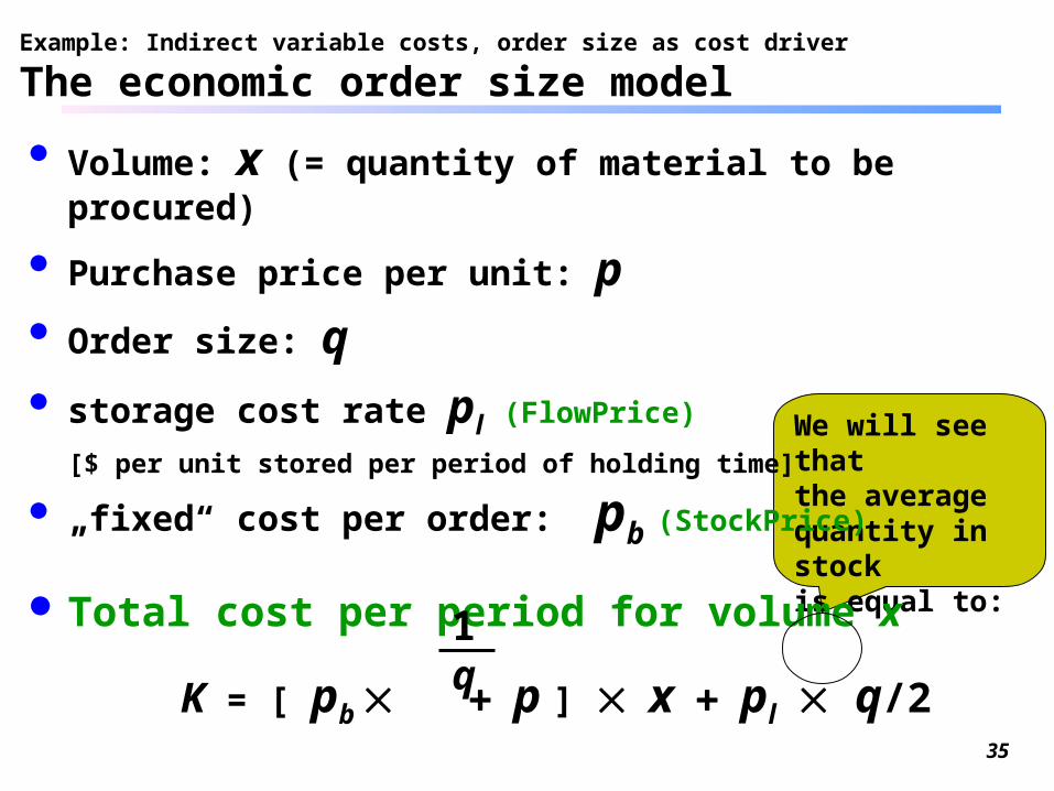
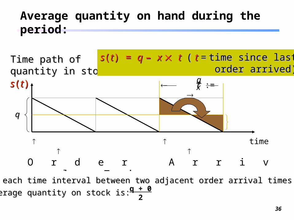
We will see thatthe average quantity in stock is equal to:
Example: Indirect variable costs, order size as cost driver
The economic order size model
Volume: x (= quantity of material to be procured)
Purchase price per unit: p Order size: q storage cost rate pl (FlowPrice)
[$ per unit stored per period of holding time]
„fixed“ cost per order: pb (StockPrice)
Total cost per period for volume x
K = [ pb p ] x pl q/21q
36
Average quantity on hand during the period:
Time path of quantity in Time path of quantity in stock:stock:
time
ss((tt))
ss((tt) = ) = q q –– x x tt (( tt = = time since lasttime since lastorder arrived)order arrived)
O r d e r A r r i v a l T i m e s
TT := :=
During each time interval between two adjacent order arrival times During each time interval between two adjacent order arrival times
the average quantity on stock is:the average quantity on stock is: q + 02
qx
37
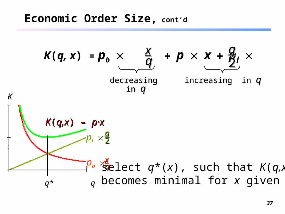
Economic Order Size, cont‘d
K(q, x) = pb p x pl xxqq
qq22
decreasing decreasing in in qq
increasing in increasing in qq
KK((q,xq,x) ) –– p·xp·x
pl qq22
pb xxqq
KK
qq*
select q*(x), such that K(q,x) becomes minimal for x given
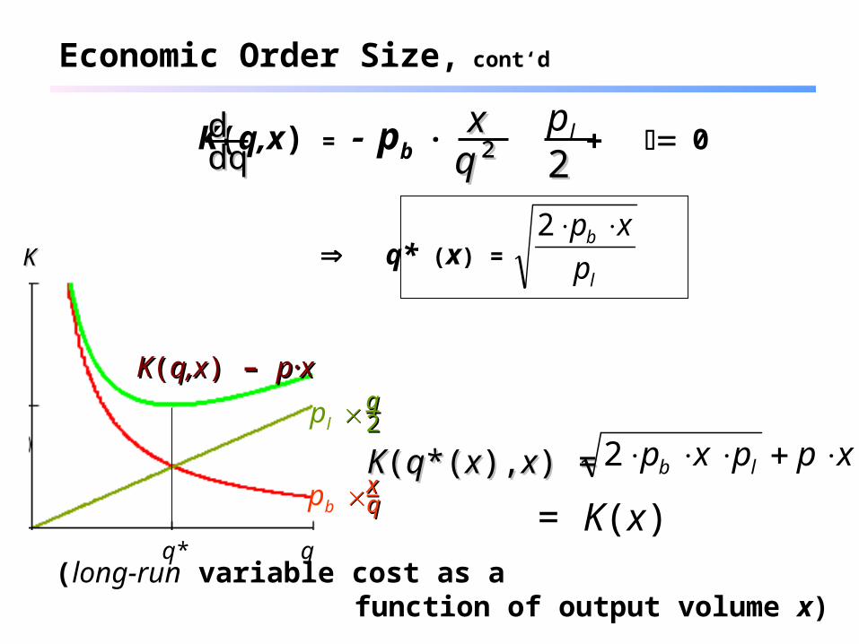
K(q,x) = pb · 0
q* (x) =
(long-run variable cost as afunction of output volume x)
xxqq²²
pl
2 2
KK((q,xq,x) ) –– p·xp·x
xxqq
KK
qq*
dddqdq
l
b
p
xp 2
KK((qq*(*(xx),),xx) = ) = xppxp lb 2
= K(x)
pl qq22
pb
Economic Order Size, cont‘d

39
Cost Functions
A cost function shows the least cost required for a given output volume x as a function of x.
The definition of a cost function depends on the scope of decision making open to Management when trying to minimize cost in determining the cost function.
When all existing cost drivers can be freely chosen, we get the long-run cost function,
otherwise we get short-run cost functions. K(x) = is a long-run
cost function. xppxp lb 2

40
Short-run cost function for the order size model
Assume order size is determined in advance according
to expected demand x, while effective demand x° may oscillate over time. Order times are determined according to
requirements x° . An order has to arrive each time store is empty.
then there is no leeway for decision left at all.
We get as a short-run cost function:
K(x°|q*(x)) = pb x°/q*(x) + pl q*(x)/2 + px°

41
Long-run versus short-run cost function for the order size model
.
x x°
K
K(x°)
K(x°|x)
Short-run cost cannot be lower than long-run cost!

42
Total Cost, Unit Cost, Marginal Cost.
Total cost: K(x)
(cost for volume x per period) Unit cost: k(x) := K(x) / x
(geometrically: the slope of a straight line through the origin and the point (x, K(x)))
Variable average cost: (K(x) – K(0)) / x
(the slope of the straight line through points (0, K(0)) and (x, K(x)))
Incremental cost: K(x + dx) K(x)
where dx denotes an increment in volume
(the slope of the straight line through the points (x, K(x)) and (x + dx, K(x + dx)))
Marginal cost: K'(x) = lim
(the slope of the tangent to the cost function at the point (x, K(x))).
K(x + dx) – K(x)dxdx 0
43
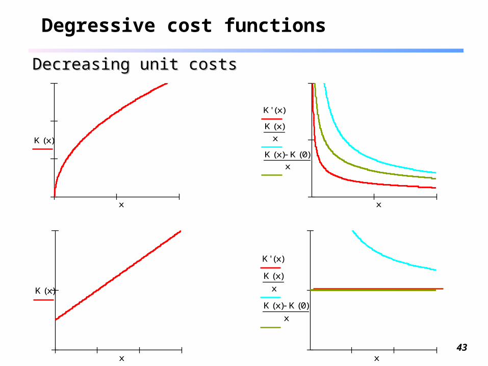
Degressive cost functions
K x( )
x
K' x( )
K x( )
x
K x( ) K 0( )x
x
K x( )
x
K' x( )
K x( )
x
K x( ) K 0( )x
x
Decreasing unit costsDecreasing unit costs
44
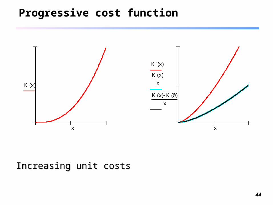
Progressive cost function
K x( )
x
K' x( )
K x( )
x
K x( ) K 0( )x
x
Increasing unit costsIncreasing unit costs

45
Regressive cost function
K x( )
x
K' x( )
K x( )
x
x
Decreasing total costsDecreasing total costs
Example: Example: Disposal costs for excess quantities of an Disposal costs for excess quantities of an intermediate product in a chemical plantintermediate product in a chemical plant
46
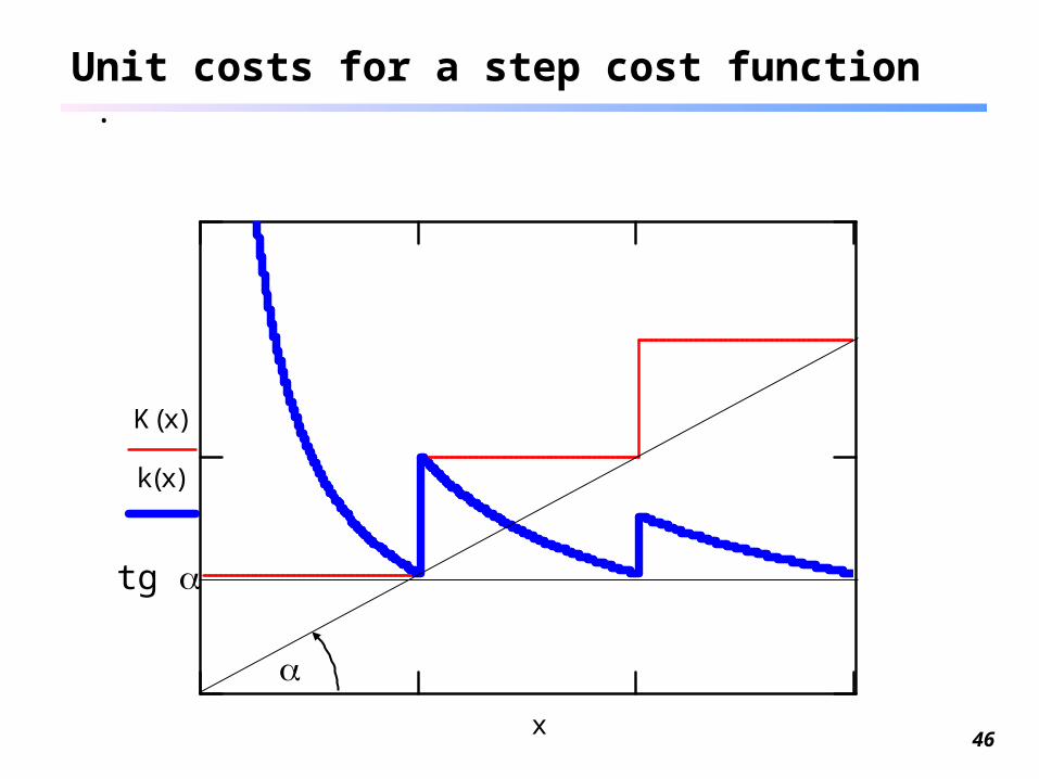
Unit costs for a step cost function.
K x( )
k x( )
x
tg

Classical cost function
K x( )
x
K' x( )
K x( )
x
K x( ) K 0( )x
x
u - shaped marginal cost function meets theu - shaped marginal cost function meets theu - shaped unit cost function in its minimum. u - shaped unit cost function in its minimum. Also the variable unit costs are u-shaped. Also the variable unit costs are u-shaped. The marginal cost function meets the variable The marginal cost function meets the variable unit cost function in its minimum, too. unit cost function in its minimum, too. Prove that!Prove that!

48
Problem 2-35 ( 5%) using Excel® recommended but not required
When you use Excel® please emphasize explanation such that the audience understands how the results come about and what they mean
Problem 2-37 (15%) Extra problem: Assume the cost function is twice
continuously differentiable. Give mathematical proofs of the following propositions (10%): if x* minimizes unit cost k then k(x*) = K‘(x*) variable average cost at x = 0 is equal to marginal cost.
CC Problems to be discussed