the low-resolution drao survey of ... - max planck societyder entwicklung von software, welche für...
TRANSCRIPT
The Low-Resolution DRAO Survey ofPolarized Emission at 1.4 GHz
Dissertationzur
Erlangung des Doktorgrades (Dr. rer. nat.)der
Mathematischen-Naturwissenschaftlichen Fakultätder
Rheinischen Friedrich-Wilhelms-Universität Bonn
vorgelegt vonMaik Wolleben
ausHannover
Bonn, 2005


Angefertigt mit Genehmigung der Mathematisch-Naturwissenschaftlichen Fakultätder Rheinischen Friedrich-Wilhelms Universität Bonn
1. Referent: Prof. Dr. U. Klein2. Referent: Prof. Dr. R. Wielebinksi
Tag der Promotion:


Zusammenfassung
Der „Low-Resolution DRAO Survey of Polarized Emission“ ist eine neue Polarisationsdurchmusterungdes Nordsternhimmels bei einer Frequenz von 1.4 GHz. Die Beobachtungen wurden mit dem „26-mTeleskop“ des Dominion Radio Astrophysical Observatory (DRAO) durchgeführt, eine Einzelantennemit einem Durchmesser von 25.6 m und einer Winkelauflösung von 36′ bei dieser Frequenz. Um absolutgeeichte Stokes U und Q Karten räumlich ausgedehnter Emissionsstrukturen zu erhalten, wurden dieDaten, mit Hilfe der Leiden/Dwingeloo Polarisationsdurchmusterung, bereinigt von Bodenstrahlung.Mittels Driftscans wurde der Himmel im Bereich zwischen −27◦ und +90◦ Deklination beobachtet.Voll gesampelte Driftscans wurden in Schritten von 1◦ bis 5◦ in Deklination gemessen und ergebeneine Abdeckung des nördlichen Himmels von 21.7%.
Diese Doktorarbeit handelt von der Durchführung und Analyse der neuen DRAO-Polarisations-Durchmusterung. Eine kurze historische Einführung, sowie eine wissenschaftliche Begründung für dieneue Durchmusterung wird gegeben. Darauf folgt eine detaillierte Beschreibung des Empfängers undder Entwicklung von Software, welche für die Durchführung der Beobachtungen notwendig war. Des-weiteren werden Fehlerquellen, sowie die absolute Eichung der Daten diskutiert. Die Ergebnisse einerersten Analyse werden präsentiert.
Diese Durchmusterung erweitert die Datenbank absolut geeichter Polarisationsbeobachtungen desNordsternhimmels. Diese Daten sind unerlässlich für die Eichung von hochaufgelösten Polarisations-beobachtungen der galaktischen Ebene, welche mit Synthese, sowie großen Einzelteleskopen durchge-führt werden, weil sie darin fehlende Informationen über ausgedehnte Strukturen liefern. Die Analysefaszinierender neuer Objekte, entdeckt in Polarisationsbeobachtungen der galaktischen Ebene, erfor-dert eine Absoluteichung der Daten. Die neue Durchmusterung des DRAO liefert Karten ausgedehnterStrukturen in Auflösung und Empfindlichkeit, welche den Anforderungen der hochaufgelösten Durch-musterungen enspricht.
Eine vorläufige Analyse der neuen DRAO-Durchmusterung enthüllt bisher unbekannte Komponen-ten polarisierter Emission, wie zum Beispiel depolarisierte Gebiete in Richtung von H -Regionen,anhand dessen die Entfernung zur „Fan“-Region, ein ausgedehntes und polarisiertes Gebiet, abgeleitetwerden kann. Desweiteren wird eine Region mit niedriger Prozentpolarisation in Richtung des erstengalaktischen Quadranten analysiert, sowie „High-Latitude Polarized Emission“ gefunden, welche alsSynchrotronemission einer magnetischen Schale interpretiert wird. Die Verbesserung des Samplingsim Vergleich zu früheren Polarisationsdurchmusterungen des nördlichen Himmels erlaubt detailliertemorphologische Studien der lokalen galaktischen Umgebung.

Abstract
The “Low-Resolution DRAO Survey of Polarized Emission” is a new polarization survey of the north-ern sky at a frequency of 1.4 GHz. The observations were carried out using the “26-m Radio Telescope”of the Dominion Radio Astrophysical Observatory (DRAO), a single-antenna with a diameter of 25.6 mand 36′ angular resolution at that frequency. The data are corrected for ground radiation, by tighten-ing to the Leiden/Dwingeloo polarization survey, to obtain absolutely calibrated Stokes U and Q mapscontaining emission structures of large spatial extend. Survey observations were carried out by driftscanning the sky between −27◦ and +90◦ declination. The fully sampled drift scans, observed in stepsof 1◦ to 5◦ in declination, result in a northern sky coverage of 21.7%.
This thesis deals with the realization and analysis of the new DRAO polarization survey. A briefhistorical introduction along with a scientific justification for the new survey is given. This is followedby a detailed description of receiver and software development necessary for carrying out the survey, aswell as a discussion of error sources and absolute calibration of the data. The first results of an initialdata analysis are presented.
This survey largely extends the data base of absolutely calibrated polarization observations of thenorthern sky. Those data bases are essential for the calibration of high-resolution polarization obser-vations made with synthesis and large single-antenna telescopes covering the Galactic plane, becausethey provide missing information on large-scale structures. The analysis of intriguing new featuresrevealed by the recent polarization observations of the Galactic plane requires an absolute calibrationof polarization data. The new DRAO survey provides maps of large-scale emission with sampling andsensitivity suited for their calibration.
A preliminary analysis of the new survey reveals previously unknown components of polarized emis-sion such as depolarized patches towards H -regions that reveal distances to the “fan”-region. Further-more, a patch of low percentage polarization towards the first quadrant of the Galaxy is analyzed.“High-Latitude Polarized Emission” is found and interpreted as synchrotron emission from a mag-netic shell. The improvement in sampling compared to previous large-scale polarization surveys of thenorthern sky allows morphological studies of the local Galactic environment in great detail.


Contents
Foreword xiii
1 Polarization Surveys 11.1 History of Polarization Surveys . . . . . . . . . . . . . . . . . . . . . . . . . . . . . . 11.2 Absolute Calibration . . . . . . . . . . . . . . . . . . . . . . . . . . . . . . . . . . . 3
1.2.1 The Role of Large-Scale Structures in Polarization Images . . . . . . . . . . . 51.2.2 The Role of Large-Scale Structures in Rotation Measures . . . . . . . . . . . . 6
1.3 Absolutely Calibrating Polarization Surveys . . . . . . . . . . . . . . . . . . . . . . . 101.3.1 Independent Absolute Calibration . . . . . . . . . . . . . . . . . . . . . . . . 101.3.2 Absolute Calibration on the Basis of Low-Resolution Data . . . . . . . . . . . 111.3.3 Absolute Calibration of Synthesis Data . . . . . . . . . . . . . . . . . . . . . 11
1.4 Scientific Justification for the 26-m Survey . . . . . . . . . . . . . . . . . . . . . . . . 111.4.1 Scope of the Project . . . . . . . . . . . . . . . . . . . . . . . . . . . . . . . 12
2 Wave Polarization in Radio Astronomy 132.1 Monochromatic Waves . . . . . . . . . . . . . . . . . . . . . . . . . . . . . . . . . . 132.2 Stokes Parameters . . . . . . . . . . . . . . . . . . . . . . . . . . . . . . . . . . . . . 152.3 Partial Polarization . . . . . . . . . . . . . . . . . . . . . . . . . . . . . . . . . . . . 162.4 Polarization Measurements . . . . . . . . . . . . . . . . . . . . . . . . . . . . . . . . 162.5 The Jones Matrix . . . . . . . . . . . . . . . . . . . . . . . . . . . . . . . . . . . . . 162.6 The Müller Matrix . . . . . . . . . . . . . . . . . . . . . . . . . . . . . . . . . . . . 172.7 Radio Emission Mechanism . . . . . . . . . . . . . . . . . . . . . . . . . . . . . . . 172.8 Faraday Rotation . . . . . . . . . . . . . . . . . . . . . . . . . . . . . . . . . . . . . 18
3 Receiving Equipment and Observations 193.1 Hardware . . . . . . . . . . . . . . . . . . . . . . . . . . . . . . . . . . . . . . . . . 19
3.1.1 The DRAO 26-m Telescope . . . . . . . . . . . . . . . . . . . . . . . . . . . 193.1.2 Cross-Correlation of Radio Signals . . . . . . . . . . . . . . . . . . . . . . . 193.1.3 The Receiver . . . . . . . . . . . . . . . . . . . . . . . . . . . . . . . . . . . 213.1.4 System Temperature . . . . . . . . . . . . . . . . . . . . . . . . . . . . . . . 263.1.5 Polarimeters . . . . . . . . . . . . . . . . . . . . . . . . . . . . . . . . . . . 273.1.6 System Adjustments . . . . . . . . . . . . . . . . . . . . . . . . . . . . . . . 30
3.2 Computer and Software . . . . . . . . . . . . . . . . . . . . . . . . . . . . . . . . . . 323.2.1 Telescope Scheduling Software . . . . . . . . . . . . . . . . . . . . . . . . . 343.2.2 Data Acquisition Software . . . . . . . . . . . . . . . . . . . . . . . . . . . . 353.2.3 Data Reduction Program . . . . . . . . . . . . . . . . . . . . . . . . . . . . . 35
3.3 Instrumental Errors – Time-Invariable . . . . . . . . . . . . . . . . . . . . . . . . . . 353.3.1 An Imperfect Feed . . . . . . . . . . . . . . . . . . . . . . . . . . . . . . . . 373.3.2 The Quadrature Hybrid . . . . . . . . . . . . . . . . . . . . . . . . . . . . . . 39
ix

Contents
3.3.3 System Gain . . . . . . . . . . . . . . . . . . . . . . . . . . . . . . . . . . . 393.3.4 The System Müller Matrix . . . . . . . . . . . . . . . . . . . . . . . . . . . . 403.3.5 Deriving the System Müller Matrix . . . . . . . . . . . . . . . . . . . . . . . 413.3.6 The Response Pattern . . . . . . . . . . . . . . . . . . . . . . . . . . . . . . . 41
3.4 Instrumental Errors – Time-Variable . . . . . . . . . . . . . . . . . . . . . . . . . . . 423.4.1 Electronic Gain . . . . . . . . . . . . . . . . . . . . . . . . . . . . . . . . . . 43
3.5 Other Errors . . . . . . . . . . . . . . . . . . . . . . . . . . . . . . . . . . . . . . . . 433.5.1 Ionospheric Effects . . . . . . . . . . . . . . . . . . . . . . . . . . . . . . . . 433.5.2 Miscellaneous . . . . . . . . . . . . . . . . . . . . . . . . . . . . . . . . . . 45
3.6 Observing . . . . . . . . . . . . . . . . . . . . . . . . . . . . . . . . . . . . . . . . . 453.6.1 Ground Radiation . . . . . . . . . . . . . . . . . . . . . . . . . . . . . . . . . 453.6.2 Observing Strategy . . . . . . . . . . . . . . . . . . . . . . . . . . . . . . . . 47
4 Data Processing and Absolute Calibration 494.1 Reduction Chain . . . . . . . . . . . . . . . . . . . . . . . . . . . . . . . . . . . . . 49
4.1.1 Radio Frequency Interference Flagging . . . . . . . . . . . . . . . . . . . . . 494.1.2 Assorting the Raw Data . . . . . . . . . . . . . . . . . . . . . . . . . . . . . 514.1.3 Electronic Gain . . . . . . . . . . . . . . . . . . . . . . . . . . . . . . . . . . 524.1.4 Pre-Calibration . . . . . . . . . . . . . . . . . . . . . . . . . . . . . . . . . . 524.1.5 Ground Radiation . . . . . . . . . . . . . . . . . . . . . . . . . . . . . . . . . 554.1.6 Gridding . . . . . . . . . . . . . . . . . . . . . . . . . . . . . . . . . . . . . 554.1.7 Solar Interference and Ionospheric Faraday Rotation . . . . . . . . . . . . . . 564.1.8 System Temperature Fluctuations . . . . . . . . . . . . . . . . . . . . . . . . 564.1.9 Interpolation . . . . . . . . . . . . . . . . . . . . . . . . . . . . . . . . . . . 584.1.10 Second Calibration . . . . . . . . . . . . . . . . . . . . . . . . . . . . . . . . 594.1.11 Final Editing . . . . . . . . . . . . . . . . . . . . . . . . . . . . . . . . . . . 59
4.2 Refinement of Temperature Scale . . . . . . . . . . . . . . . . . . . . . . . . . . . . . 604.3 Error Analysis . . . . . . . . . . . . . . . . . . . . . . . . . . . . . . . . . . . . . . . 60
4.3.1 The System Müller Matrix . . . . . . . . . . . . . . . . . . . . . . . . . . . . 614.3.2 Response . . . . . . . . . . . . . . . . . . . . . . . . . . . . . . . . . . . . . 634.3.3 Side Lobe Polarization . . . . . . . . . . . . . . . . . . . . . . . . . . . . . . 634.3.4 Noisy Reference Values and Congruence Radius . . . . . . . . . . . . . . . . 644.3.5 Repeatability of Drift Scans . . . . . . . . . . . . . . . . . . . . . . . . . . . 644.3.6 Final Error . . . . . . . . . . . . . . . . . . . . . . . . . . . . . . . . . . . . 66
5 Survey Maps 67
6 Improved Calibration of Effelsberg Medium Latitude Survey 796.1 Introduction . . . . . . . . . . . . . . . . . . . . . . . . . . . . . . . . . . . . . . . . 796.2 Method . . . . . . . . . . . . . . . . . . . . . . . . . . . . . . . . . . . . . . . . . . 796.3 Discussion . . . . . . . . . . . . . . . . . . . . . . . . . . . . . . . . . . . . . . . . . 80
7 Initial Data Analysis 857.1 Introduction . . . . . . . . . . . . . . . . . . . . . . . . . . . . . . . . . . . . . . . . 85
7.1.1 Large-Scale Morphology of Polarized Emission . . . . . . . . . . . . . . . . . 867.1.2 Local Interstellar Medium . . . . . . . . . . . . . . . . . . . . . . . . . . . . 89
7.2 Most Pronounced Objects in Polarization . . . . . . . . . . . . . . . . . . . . . . . . 917.2.1 North-Polar Spur and Loop I . . . . . . . . . . . . . . . . . . . . . . . . . . . 917.2.2 The Fan-Region . . . . . . . . . . . . . . . . . . . . . . . . . . . . . . . . . . 92
x

Contents
7.3 Newly Detected Polarization Features . . . . . . . . . . . . . . . . . . . . . . . . . . 947.3.1 Depolarizing H -Regions . . . . . . . . . . . . . . . . . . . . . . . . . . . . 947.3.2 The Depolarization Patch . . . . . . . . . . . . . . . . . . . . . . . . . . . . . 967.3.3 High-Latitude Polarized Emission . . . . . . . . . . . . . . . . . . . . . . . . 101
7.4 Results and Discussion . . . . . . . . . . . . . . . . . . . . . . . . . . . . . . . . . . 102
8 Summary and Conclusion 1058.1 Major Contributions . . . . . . . . . . . . . . . . . . . . . . . . . . . . . . . . . . . . 1058.2 Future Work . . . . . . . . . . . . . . . . . . . . . . . . . . . . . . . . . . . . . . . . 106
Müller Matrix Elements 107
Bibliography 107
List of Tables 113
List of Figures 116
Acknowledgements 117
Curriculum Vitae 119
xi

Contents
xii

ForewordThe polarization of Galactic synchrotron emission is being measured since more than 40 years at fre-quencies from 100 MHz to 1 GHz and higher, involving different kinds of receivers and telescopes.With the availability of high-resolution polarization data obtained during the last decade, numerousnew objects and features that can only be seen in polarization are detected. A new generation of polar-ization surveys made with large single-antenna and synthesis telescopes clearly opens a new windowfor the investigation of the magneto-ionic medium of our Galaxy.
For the study of diffuse Galactic emission the absolute calibration of polarimetric data by incorpo-ration of large-scale emission (zero-spacings) is of vital importance. Zero-spacings are missing in ob-servations made with synthesis and large single-antenna telescopes, because of insensitivity of interfer-ometers to large-scale emission or confusion with ground and stray radiation in case of single-antennatelescopes. Hence, a new absolutely calibrated survey with sufficient high sensitivity is required to al-low correction of actual high-resolution data. The realization and analysis of such a survey is describedin the present thesis.
Starting with my first year for a doctorate at the Dominion Radio Astrophysical Observatory (DRAO)in Penticton, Canada, I found myself facing a 26-m telescope that had never been used for polarimet-ric observations before; with a receiver that was not intended for observations of linear polarization.Moreover, the backend device, a continuum polarimeter shipped from the Max-Planck Institut für Ra-dioastronomie in Bonn (MPIfR), was waiting to be “plugged in”. Since no experience using this tele-scope for polarization observations existed, this PhD project gave me the opportunity to gain insightinto many different aspects of performing a polarization survey such as technical, observational, andcalibration issues.
One year (May 2002 - May 2003) was dedicated for polarimetric work at the DRAO 26-m Telescope,including survey observations. Almost the first half of this year I spent making the “26-m” capable ofmeasuring linear polarization. Prior to observing, two things had to be developed at the same time. Thereceiver required modifications to allow measurements of linear polarization and software needed tobe written to control the backend devices, data acquisition, and recording. After making sure that hard-and software worked well, an observing scheme was developed and survey observations could start.
Back at the MPIfR, a data processing and reduction chain had to be set up to handle and calibrate theenormous amount of data collected during 7 months of observing. The results are absolutely calibratedStokes U and Q maps of the northern sky. Although not fully sampled, these maps consist of 100 timesmore data points than provided by the Leiden/Dwingeloo polarization survey (observed between 1961and 1966), while covering a larger area of the sky.
It was soon obvious that the new survey not only provides information about low spatial frequenciesfor the calibration of high-resolution data, but also yields new aspects of the polarized sky. Therefore,an analysis of the new data is presented and first results are discussed.
In the first part (Chapters 1 and 2) of this thesis, the scientific justification for the new polarizationsurvey is discussed, and the meaning and importance of “absolute calibration” for studies of polarizedemission are specified. Some historical aspects are also given. Furthermore, the reader is introduced tothe basic formalism of wave polarization that is used in this thesis.
The second part (Chapters 3, 4, and 5) deals with all aspects of undertaking the survey observations,starting with a description of the receiver and necessary modifications, software that needed to bewritten, error sources, and the data processing and calibration. Survey observations were done by
xiii

Foreword
drift scanning. Additional measurements were made for calibration purposes and the determination ofground radiation profiles. The path of the data from the receiver to the final polarization maps will bedescribed.
In the third part (Chapters 6 and 7) a study of the new polarization data is presented. This startswith a description of the large-scale distribution of polarized emission. Known Galactic objects areidentified as well as new features outlined. Polarized emission at high Galactic latitudes is interpretedas synchrotron emission from a magnetic shell. Depolarization of diffuse polarized emission, causedby H -regions, is used to derive lower limits on the distance to the “fan”-region, a spatially extended,intense patch of highly polarized emission.
Finally, a conclusion and outlook are given in the last part (Chapter 8). The survey presented in thisthesis has a sky coverage of 21.7% of the surveyed region. Meanwhile (by March 2005), a coverageof more than 43% has been achieved in the course of ongoing survey observations. These data will bemade available via web interface as explained in the last Chapter.
xiv

List of acronyms frequently used:Low-Resolution DRAO Survey of Polarized Emission 26-m Survey
Canadian Galactic Plane Survey CGPSEffelsberg Medium Latitude Survey EMLS
High Latitude Polarized Emission HLPELeiden-Dwingeloo Survey of Polarized Emission at 1.4 GHz LDS

Foreword
xvi
1 Polarization Surveys
This chapter gives a brief review of polarization surveys, a discussion of absolute calibration inpolarimetry, and the justification for the new polarization survey. The first polarization surveysprovided polarized brightness temperatures for large areas of the sky. But the data are onlysparsely sampled, resulting in low angular resolution. In recent years, a new generation of polar-ization surveys covering the Galactic plane has been initiated and will provide fully sampled mapsof high angular resolution. High-resolution surveys, however, lack large-scale structures (zero-spacings) necessary for an absolute calibration. This information must come from low-resolutionsurveys such as the new DRAO polarization survey presented in this thesis.
1.1 History of Polarization Surveys
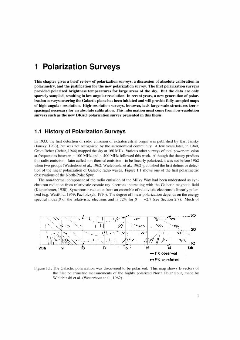
In 1933, the first detection of radio emission of extraterrestrial origin was published by Karl Jansky(Jansky, 1933), but was not recognized by the astronomical community. A few years later, in 1940,Grote Reber (Reber, 1944) mapped the sky at 160 MHz. Various other surveys of total power emissionat frequencies between ∼ 100 MHz and ∼ 400 MHz followed this work. Although the theory predictsthis radio emission – later called non-thermal emission – to be linearly polarized, it was not before 1962when two groups (Westerhout et al., 1962; Wielebinski et al., 1962) published the first definitive detec-tion of the linear polarization of Galactic radio waves. Figure 1.1 shows one of the first polarimetricobservations of the North-Polar Spur.
The non-thermal component of the radio emission of the Milky Way had been understood as syn-chrotron radiation from relativistic cosmic ray electrons interacting with the Galactic magnetic field(Kiepenheuer, 1950). Synchrotron radiation from an ensemble of relativistic electrons is linearly polar-ized (e.g. Westfold, 1959; Pacholczyk, 1970). The degree of linear polarization depends on the energyspectral index β of the relativistic electrons and is 72% for β = −2.7 (see Section 2.7). Much of
Figure 1.1: The Galactic polarization was discovered to be polarized. This map shows E-vectors ofthe first polarimetric measurements of the highly polarized North Polar Spur, made byWielebinski et al. (Westerhout et al., 1962).
1
1 Polarization Surveys
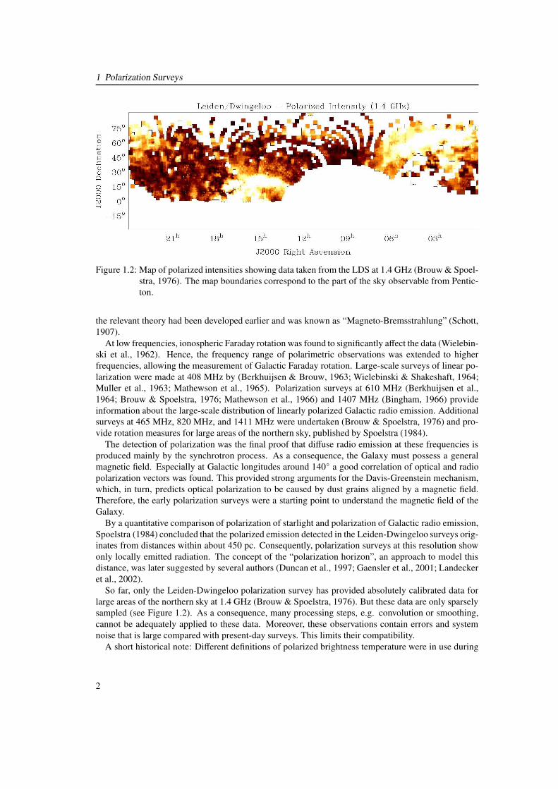
Figure 1.2: Map of polarized intensities showing data taken from the LDS at 1.4 GHz (Brouw & Spoel-stra, 1976). The map boundaries correspond to the part of the sky observable from Pentic-ton.
the relevant theory had been developed earlier and was known as “Magneto-Bremsstrahlung” (Schott,1907).
At low frequencies, ionospheric Faraday rotation was found to significantly affect the data (Wielebin-ski et al., 1962). Hence, the frequency range of polarimetric observations was extended to higherfrequencies, allowing the measurement of Galactic Faraday rotation. Large-scale surveys of linear po-larization were made at 408 MHz by (Berkhuijsen & Brouw, 1963; Wielebinski & Shakeshaft, 1964;Muller et al., 1963; Mathewson et al., 1965). Polarization surveys at 610 MHz (Berkhuijsen et al.,1964; Brouw & Spoelstra, 1976; Mathewson et al., 1966) and 1407 MHz (Bingham, 1966) provideinformation about the large-scale distribution of linearly polarized Galactic radio emission. Additionalsurveys at 465 MHz, 820 MHz, and 1411 MHz were undertaken (Brouw & Spoelstra, 1976) and pro-vide rotation measures for large areas of the northern sky, published by Spoelstra (1984).
The detection of polarization was the final proof that diffuse radio emission at these frequencies isproduced mainly by the synchrotron process. As a consequence, the Galaxy must possess a generalmagnetic field. Especially at Galactic longitudes around 140◦ a good correlation of optical and radiopolarization vectors was found. This provided strong arguments for the Davis-Greenstein mechanism,which, in turn, predicts optical polarization to be caused by dust grains aligned by a magnetic field.Therefore, the early polarization surveys were a starting point to understand the magnetic field of theGalaxy.
By a quantitative comparison of polarization of starlight and polarization of Galactic radio emission,Spoelstra (1984) concluded that the polarized emission detected in the Leiden-Dwingeloo surveys orig-inates from distances within about 450 pc. Consequently, polarization surveys at this resolution showonly locally emitted radiation. The concept of the “polarization horizon”, an approach to model thisdistance, was later suggested by several authors (Duncan et al., 1997; Gaensler et al., 2001; Landeckeret al., 2002).
So far, only the Leiden-Dwingeloo polarization survey has provided absolutely calibrated data forlarge areas of the northern sky at 1.4 GHz (Brouw & Spoelstra, 1976). But these data are only sparselysampled (see Figure 1.2). As a consequence, many processing steps, e.g. convolution or smoothing,cannot be adequately applied to these data. Moreover, these observations contain errors and systemnoise that is large compared with present-day surveys. This limits their compatibility.
A short historical note: Different definitions of polarized brightness temperature were in use during
2

1.2 Absolute Calibration
the first decades of radio polarimetry. A unified scheme based on Stokes parameters was proposedby Berkhuijsen (1975). To convert brightness temperatures stated in the various early surveys to theunified system, conversion factors ranging from 0.5 to 1.3 needed to be applied. Berkhuijsen noted thatit is often difficult to determine these factors after so many years, because of the lack of observationaldetails published.
Systematic polarization observations experienced a renaissance during the past several years. Withthe development of new receivers, surveys of the Galactic plane at higher radio frequencies (e.g.: Junkeset al., 1986, at 2.7 GHz; Duncan et al., 1997, at 2.3 GHz) were made and revealed surprising struc-tures in polarization. Low-frequency polarimetric mapping with synthesis telescopes (e.g. Wieringaet al., 1993, at 350 MHz) confirms the presence of numerous structures and objects detectable only inpolarization.
For the study of these objects and the magneto-ionic properties of the interstellar medium, polariza-tion surveys with high sensitivity and resolution mainly covering the Galactic plane are currently beingcarried out. Observations for the Effelsberg Medium Latitude Survey (|b| ≤ 20◦, Uyanıker et al, 1998,1999, Reich at al., 2004) at 1.4 GHz have just been finished. The International Galactic Plane Survey(IGPS, |b| . 5◦), a major undertaking of mapping the Galactic plane with different telescopes at variouswavelengths, provides polarization data at 1.4 GHz obtained with the DRAO synthesis telescope. Inthe southern hemisphere the Australia Telescope Compact Array is mapping the Galactic plane (SGPS,|b| ≤ 1◦, Dickey et al., 1999) also at 1.4 GHz.
Compared with the early polarization observations, sensitivity and resolution of the new surveyshas improved due to utilization of large single-antenna and synthesis telescopes equipped with cooledreceivers. But large-scale emission is missing in observations made with these telescopes, becauseof either insensitivity of interferometers to low spatial frequencies or the baseline setting procedure1
in single-antenna mapping. Whenever required for the analysis, such data must be augmented withabsolutely calibrated data to account for the missing flux and structures. These absolutely calibrateddata can have low angular resolution because they only add spatially extended emission.
1.2 Absolute Calibration
Measuring absolute intensities of radio signals is difficult, because the radio signal from the source inthe sky is received through the antenna and the receiving system which contribute noise and amplifyit. Unless the antenna is of simple design so that its gain can be calculated to good precision, the exactgain of the system is unknown. Such simple antennas are horns, and total power observations are beingcalibrated by adjusting their flux density or temperature scale to the absolute intensities derived bymeasurements with horn antennas (e.g. Howell & Shakeshaft, 1966).
The polarized-brightness-temperature scales of the early polarization surveys are calibrated againsta number of “standard” calibration points. The polarization degree and angle of these standard pointswere measured with receivers for which the gain in total power was known. In Figure 1.3 the polarizedintensities of two such calibration points frequently used for the early surveys are plotted. It can be seenthat, with different telescopes, different temperatures were obtained, partly because different definitionsof polarized brightness temperature were used.
The receiving system introduces noise and noise is also received through the side lobes of the tele-scope. This noise is of the same kind as the signal from the radio source and can therefore not bedistinguished. Whereas receivers are usually temperature controlled and stable enough to produce a
1Baseline setting means that a linear “baseline” (first order polynomial) is fitted through the start and end of each subscan andis subsequently subtracted. By this, the edges of maps are set to zero, which removes ground and spillover noise but alsolarge-scale emission on scales equal or greater than the map size.
3

1 Polarization Surveys
Figure 1.3: Diagram shows polarized brightness temperatures of two frequently used calibration points,derived with different telescopes at various frequencies (from Berkhuijsen, 1975).
relatively constant level of receiver noise, the amount of noise received through the far side lobes –mainly ground radiation – varies as the telescope is tracking a source. This leads to the problem ofseparating the sky from ground radiation.
If telescope movement is small and hence fluctuations of the ground radiation negligible withina subscan, ground radiation offsets are removed by baseline fitting to good approximation, as donefrequently at the Effelsberg 100-m telescope. The obvious drawback of this method is the suppressionof large-scale emission that exceeds the size of the map.
The level of ground radiation, however, can be large, because the side lobes extend to very large dis-tances from the main beam and signals are received even from the back side of the telescope. Althoughsuppression of side lobes is usually better than 30 dB, their integrated flux over 4π can be higher thanthe actual flux received from a source. Therefore the side lobes cannot be neglected in case of absolutemeasurements.
An absolute calibration of radio data consists of two principal steps. First, a scaling factor must bedetermined that converts the arbitrary intensity scale of the raw data into physical units. This factor canbe found, for example, by mapping standard calibrators (compact sources of known flux) and referringthe measured flux to the standard fluxes of these calibrators. Also possible is the injection of calibrationsignals into the receiver instead of mapping standard calibrators. Second, to measure absolute fluxes,the received signal must be separated into noise contributions from the receiver, ground, atmosphere,
4
1.2 Absolute Calibration
and the actual sky signal. If ground radiation has been removed by baseline subtraction missing large-scale emission must be replaced.
Missing large-scale structures must also be replaced in observations made with aperture synthesistelescopes if absolute fluxes are required. Incomplete coverage of the visibility plane leads to missinginformation in the image plane. This is known as the missing-zero-spacing problem and means thata synthesis telescope is insensitive to emission structures larger than the angle corresponding to itsshortest spacing.
Other than in total power maps, in which pixel values are scalar quantities, polarimetry deals withvectors. Each pixel in a polarimetric map is a vector that has a length and direction. The recovery ofzero-spacings or missing large-scale structures in polarimetric observations always means to correctvectors. Therefore, missing spatial information can affect the data in a much more complicated waythan in total power. Its effect on polarized intensity and angle as well as on rotation measures will bediscussed now.
1.2.1 The Role of Large-Scale Structures in Polarization Images
Missing large-scale structures can have a significant impact on the morphological information containedin polarization images. The polarized intensity is defined by PI =
√
U2 + Q2. Hence, PI is always apositive quantity and, because it is calculated via Stokes U and Q squared, highly sensitive to offsets inU and Q due to large-scale emission. Correction of offsets can turn an object of high polarized intensityinto one of seemingly depressed polarized emission relative to its surroundings, and vice versa. In thesame way the polarization angle is affected. Moreover, depending on the large-scale structure that ismissing, the position of structures can be shifted.
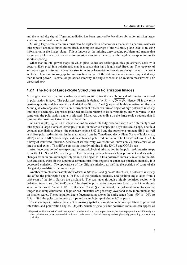
As an example, Figure 1.4 displays maps of polarized intensity, observed with three different types oftelescopes: a large-diameter telescope, a small-diameter telescope, and a synthesis telescope. The fieldcontains two distinct objects: the planetary nebula SH2-216 and the supernova remnant HB 9, as wellas diffuse polarized emission. In the maps taken from the Canadian Galactic Plane Survey (Taylor et al.,2003) and the EMLS, both objects show enhanced polarized emission. The Low-Resolution DRAO-Survey of Polarized Emission, because of its relatively low resolution, shows only diffuse emission oflarge spatial extent. This diffuse emission is partly missing in the EMLS and CGPS maps.
After incorporation of zero-spacings the morphological information in the polarized intensity mapsfrom the CGPS and EMLS changes. The planetary nebula becomes less prominent and its naturechanges from an emission-type2 object into an object with less polarized intensity relative to the dif-fuse emission. Parts of the supernova remnant turn from regions of enhanced polarized intensity intodepressed emission. The appearance of the diffuse emission, as well as the position of some of theelongated, canal-like structures changes.
Another example demonstrates how offsets in Stokes U and Q create structures in polarized intensityand affect the polarization angle. In Fig. 1.5 the polarized intensity and position angle taken from adrift scan of the 26-m Survey are displayed. The scan goes through a highly polarized region withpolarized intensities of up to 450 mK. The absolute polarization angles are close to ϕ ≈ 45◦ with onlysmall variations of ∆ϕ ≈ ±10◦. If offsets in U and Q are removed, the polarization vectors are nolonger absolutely calibrated. The polarized intensities are generally lower and show more fluctuationson smaller scales. The polarization angle fluctuates almost over the entire range from −90◦ to +90◦. AtR.A. = 89◦, the polarized intensity drops and an angle jump of almost 90◦ appears.
These examples illustrate the effect of missing spatial information on the interpretation of polarizedintensities and polarization angles. Objects, which originally emit polarized radiation can appear as
2Expressions like “emission” and “absorption” must be used with care in polarization, because superposition of differently ro-tated polarization vectors can result in enhanced or depressed polarized intensity without physically generating or obstructingradiation.
5
1 Polarization Surveys
Figure 1.4: The effect of missing spatial information shown on a 7◦ × 7◦ large field centred at l = 158◦,b = 1◦, observed with three different telescopes. In the top row from left to right: the 26-mSurvey (single-antenna), the EMLS (single-antenna), and the CGPS (synthesis telescope).The bottom row shows the combinations of spatial information taken from the EMLS and26-Survey, and from all three surveys. The images contain the supernova remnant HB 9(upper left, ∼ 2◦ in size) and the planetary nebula SH2-216 (close to centre, ∼ 1◦ in size).
minima, whereas depolarizing Faraday screens3 may be observed as enhancements in polarized inten-sity. The same holds for the angle that may show fluctuations without physical equivalent. In studiesof diffuse polarized emission an absolute calibration is therefore mandatory; only in studies of distinctobjects an absolute calibration may not be necessary.
1.2.2 The Role of Large-Scale Structures in Rotation Measures
The rotation measure (RM) describes the change of polarization angle as a function of frequency (seeSection 2.8). Since the angle is very sensitive to the calibration, as seen in the previous section, howdo missing offsets in Stokes U and Q affect RMs? The question will be discussed now whether thepolarization angles must be absolutely calibrated or if relative angle variations at different frequenciesalready reveal true rotation measures. This question is of particular interest for RM-studies of diffusepolarized emission.
In the following two different cases will be discussed. The first case describes a Faraday rotatinglayer situated between a source of polarized emission – the background layer – and the observer (case-
3A Faraday screen may be an object or layer that causes Faraday rotation.
6

1.2 Absolute Calibration
60 80 100R.A. (deg)
0
150
300
450
PI (m
K)
60 80 100R.A. (deg)
-90
-60
-30
0
30
60
90
PA (d
eg)
Figure 1.5: The effect of missing large-scale structures: The left panel shows the polarized intensity(PI) taken from a survey drift scan at 57.◦5 declination with large-scale structures (thickline) and without (thin line). The right panel displays the same for the polarization angle(PA). For this example the large-scale structure is approximated by averaging of Stokes Uand Q over the right ascension interval displayed.
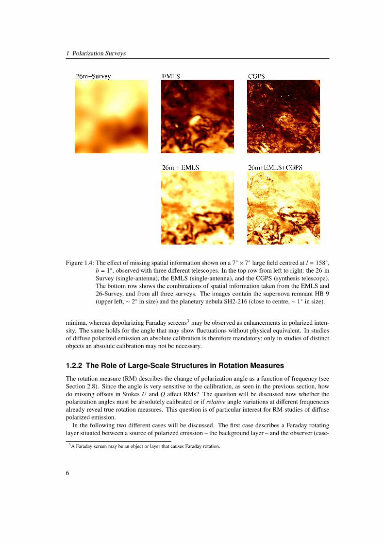
1, Fig 1.6). This case can be applied to observed emission from distant, compact objects, which can beseparated from foreground emission. The second case describes the diffuse Galactic emission in whichFaraday rotated background is observed in superposition with unrotated foreground (case-2, Fig 1.6).
Throughout the discussion B1,2 denote background polarization vectors and F1,2 foreground vectorsat frequencies ν1 and ν2. B and F are itself composed of vectors:
B1,2 = b1,2 + β1,2F1,2 = f1,2
︸︷︷︸
offset
+ ε1,2︸︷︷︸
fluctuations
, (1.1)
for which b and f shall represent offsets (large-scale structure), and β and ε denote fluctuations (small-scale structure) in polarized emission. This distinction will allow the analysis of differences in ab-solutely calibrated vectors (|b1,2| > 0, |f1,2| > 0) and those with missing zero-spacings (|b1,2| = 0,|f1,2| = 0).
The observed angle ϕFR between the polarization vectors at frequencies ν1 and ν2 is
ϕFR = ϕ1 − ϕ2 = c2
1ν21− 1ν22
RMobs (1.2)
which, if the angle difference is measured, allows the calculation of RMobs. For simplification, thex-components of the foreground and background vectors are assumed to be zero at frequency ν1, whichonly means that the vectors are lined up along the y-axis at that frequency (see Figure 1.7). Hence,the position angle of the polarization vector observed at frequency ν2 is proportional to the observedrotation measure: RMobs ∝ ϕ2.
In the first case, the background vector B is Faraday rotated. The observed polarization vector atfrequency ν2 is the vector sum of Faraday rotated offset b1 and Faraday rotated small-scale structureβ1. Its x- and y-components are:
B2,x = b2,x + β2,x = (b1,x + β1,x) cosϕFR + (b1,y + β1,y) sinϕFRB2,y = b2,y + β2,y = −(b1,x + β1,x) sinϕFR + (b1,y + β1,y) cosϕFR.
(1.3)
7
1 Polarization Surveys
RM
BACKGROUND OBSERVER
FOREGROUND OBSERVERBACKGROUND
RM
rad/m 2RMobs
PI-BACKGROUND150
200
250
PI-FOREGROUND ROTATION MEASURE-5
0
5
10
with offsetwithout offset
CASE 2
CASE 1
mK
x
x x x
BACKGROUNDPOLARIZED INTENSITY
FOREGROUNDPOLARIZED INTENSITY
Figure 1.6: The two cases are illustrated: Case-1 with background emission and Faraday rotating layerand case-2 with foreground, background and Faraday rotating layer in between. For the sec-ond case, the graphs show the adopted distribution of polarized intensity for foreground andbackground layer as well as the resulting rotation measure simulated for observations witha telescope sensitive to the large-scale structure (with offsets) and one that is not sensitiveto large-scale emission (without offset). This calculation assumes: two observing frequen-cies at 1400 and 1410 MHz, equal polarization angles of foreground and background withx-components of zero at both frequencies, and RM = 5 rad m−2. Zero spacings (offsets)are removed by subtracting the average of Stokes U and Q before calculating the rotationmeasure.
8
1.2 Absolute Calibration
b1
β1
b2
β2ε 2
f1
ε 1
f 2
β1
b1b2ϕ
2
ϕ2
ϕFR
ϕFR =
=
β2
=
y y
x x
CASE 2CASE 1
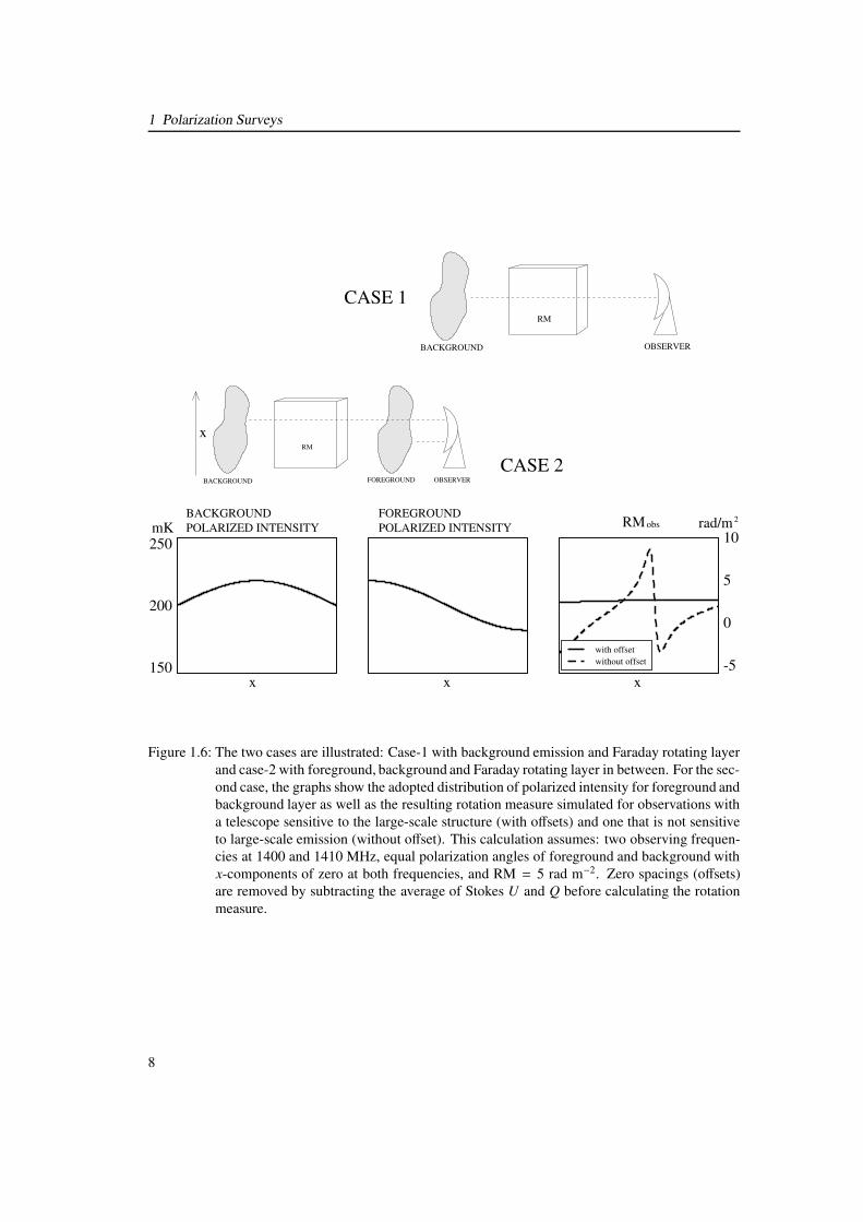
Figure 1.7: Vectors in the two cases: In case-1 only background emission exists. The vector b1 + β1 isrotated against b2+β2 because of Faraday rotation. The observed angle ϕ2 reveals the correctrotation measure (ϕ2 = ϕFR). In case-2, the rotated background (b2+β2) is superimposed onan unrotated foreground ( f1 + ε1). The observed angle ϕ2 gives a smaller rotation measurethan in case-1 (ϕ2 , ϕFR).
The polarization vector observed at ν1 is assumed parallel to the y-axis so that b1,x = β1,x = 0. There-fore, the position angle of B2 relative to the y-axis is proportional to the observed rotation measure. Itstangens is given by
tanϕ2 =B2,x
B2,y=
(b1,y + β1,y) sinϕFR
(b1,y + β1,y) cosϕFR= tanϕFR ⇒ ϕ2 = ϕFR. (1.4)
It follows that the angle difference between polarization vectors observed at frequency ν1 and ν2 revealRM correctly whether derived from absolutely calibrated data or from data with missing zero-spacings.
In case-2, which includes foreground emission, the observed polarization vector at frequency ν2 isthe composition of unrotated foreground F1 and rotated background. According to Fig. 1.6:
F2,x + B2,x = f1,x + ε1,x + (b1,x + β1,x) cosϕFR + (b1,y + β1,y) sinϕFR
F2,y + B2,y = f1,y + ε1,y − (b1,x + β1,x) sinϕFR + (b1,y + β1,y) cosϕFR.(1.5)
Again, with the simplification that all x-components are zero at frequency ν1, the tangens of the positionangle of the polarization vector at frequency ν2 is
tanϕ2 =(b1,y + β1,y) sinϕFR
f1,y + ε1,y + (b1,y + β1,y) cosϕFR. (1.6)
Here, ϕ2 becomes a function of the foreground vectors:
ϕ2 = arctan(
2 (b1,y+β1,y) tan ϕFR2
f1,y+ε1,y+b1,y+β1,y+ f1,y tan2 ϕFR2 +ε1,y tan2 ϕFR
2 −b1,y tan2 ϕFR2 −β1,y tan2 ϕFR
2
)
⇒ ϕ2 , ϕFR | f1,y| > 0,(1.7)
which, if the foreground ( f1,y, ε1,y) is zero, becomes ϕ2 = ϕFR and case-2 transforms into case-1.These results can be summarized as follows: Without foreground emission, absolute and relative po-
larization angles result in equal RM. But if polarized foreground emission is present, the RMs derivedfrom data with missing offsets can largely differ from RMs calculated on the basis of absolutely cali-brated data. In this case, RMs can be smaller or larger than the absolute rotation measures, depending
9
1 Polarization Surveys
on the foreground polarization. As case-2 applies to the interstellar medium it is highly desirable to useabsolutely calibrated data for rotation measure studies of the diffuse polarized emission.
1.3 Absolutely Calibrating Polarization Surveys
Different types of telescopes require different methods for the absolute calibration of polarization ob-servations. With small-diameter telescopes (e.g. Dwingeloo 25-m, DRAO 26-m, etc.), at frequenciesbetween ∼ 100 MHz and ∼ 10 GHz, it may not be possible to find polarized compact sources suit-able for the calibration, because, if observed with a small telescope, the commonly used calibrators aretoo weak to be detectable against the diffuse polarized background. On the other hand, large-aperturetelescopes (e.g. Effelsberg 100-m, synthesis arrays) have the resolution to map compact sources withhigh response, which allows accurate determination of the relative temperature or flux density scale,but usually do not preserve absolute fluxes.
This section describes how polarimetric data can be absolutely calibrated. Three types of abso-lute calibration are necessary in practise: 1. an independent absolute calibration of single-antennaobservations, mostly applied to small-diameter telescopes (e.g. LDS); 2. an absolute calibration ofsingle-antenna observations on the basis of low-resolution data (e.g. Effelsberg 100-m combined withStockert 25-m); and 3. the adding of zero-spacings and offsets to synthesis data.
1.3.1 Independent Absolute Calibration
For independent measurements of absolute antenna temperatures the relative temperature scale mustbe determined, as well as the noise contributions from the receiver, ground, atmosphere and the sourcedisentangled. As instances of the method, two polarization surveys are mentioned here:
• For the Leiden-Dwingeloo polarization survey at 820 MHz (Berkhuijsen, 1971) the relative tem-perature scale was obtained by comparing the recorded intensities with calibrated noise signalsadded to the sky signal during the observations. The equivalent temperature of the calibrationsignals was known, and loads in liquid nitrogen at a temperature of 78 K were used as reference.Data were corrected for ground radiation by subtracting an empirical stray radiation model.
• For the LDS reference points of known polarized intensity and angle were observed with rotatingdipoles for the calibration of the system. During measurement the dipole was rotated by 360◦,which causes the polarization vector to rotate twice in the U-Q plane, while the length of thevector, the polarized intensity, remains constant. The recorded outputs consisted of double sinecurves from which Stokes U and Q could be derived. These sine curves were corrected forground radiation on the basis of ground radiation profiles.
Much effort went into the calculation and measurement of ground radiation profiles for these surveys.At telescopes such as the Dwingeloo or DRAO 26-m, spillover and ground radiation dominates thesignal and must be known precisely. The problem is the strong dependence on elevation and azimuth,which is the result of the telescopes’s response pattern and the surrounding landscape. Time-variabilitymakes correction for ground radiation more complicated. This is why precise calculation is difficult andground radiation profiles are usually measured by making sweeps in elevation from horizon to zenith.
To correct for instrumental polarization, the response of the receiving system to unpolarized radiation– the response or antenna pattern – must be measured for all Stokes parameters. At small telescopesand frequencies around 1 GHz or less, often Cassiopeia-A and the Sun are the only sources that arestrong enough to be used for the mapping of the response pattern. In many studies, the correction ofmain-beam instrumental polarization is sufficient. But even compact sources with lower intensities canincrease instrumental polarization if observed through the side lobes.
10

1.4 Scientific Justification for the 26-m Survey
1.3.2 Absolute Calibration on the Basis of Low-Resolution Data
Whereas the measurement of ground radiation is time consuming, available observing time at large-diameter telescopes (e.g. Effelsberg 100-m) is usually limited. Moreover, ground radiation is time-variable and the measured profiles may not be accurate enough; not a problem if enough observingtime is available to either measure ground radiation profiles frequently or set up an observing schemethat allows software correction. Therefore, observations with large single-antenna telescopes can of-ten not adequately be corrected for ground radiation, and large-scale structures must be recovered bycomparison with low-resolution surveys.
Especially the Effelsberg 100-m telescope is located in a valley with surrounding hills, which intro-duces a strong dependence of the ground radiation on azimuth. Other large-diameter telescopes suchas the Parkes telescope, the Green-Bank telescope or Jodrell Bank have flatter surroundings and shouldtherefore show smaller azimuthal dependencies at low elevation.
1.3.3 Absolute Calibration of Synthesis Data
For observations obtained with aperture synthesis telescopes, various different approaches and datareduction packages can be used for the incorporation of zero-spacings. Some operate in the Fourierdomain and merge single-antenna and synthesis data involving tapering of the Fourier plane (linearmethod), and some use both data sets for a joint deconvolution (non-linear method). Mosaicing canalso help to recover short spacings.
In interferometric observations, ground radiation is “filtered out” by the cross-correlation, becauseeach individual antenna of an array receives its own ground radiation and ground radiation signals ofpairs of antennas are uncorrelated. Therefore, it is usually not necessary to correct for ground andspillover noise in continuum observations made with synthesis telescopes.
1.4 Scientific Justification for the 26-m Survey
For studies of diffuse polarized emission the data must be absolutely calibrated to contain low spatialfrequencies correctly. So far, the only data base of absolutely calibrated polarization data usable for theabsolute calibration of the recent 1.4 GHz polarization surveys is the LDS, consisting of measurementsof individual, well calibrated pointings. But these data are undersampled. In many areas pointings areseveral degrees apart and often only a small number of data points can be used for calibration. Reich &Wielebinski (2000) therefore suggested new low-resolution observations that should exceed the LDSbut include its absolute calibration. Their publication provides the groundwork for the 26-m Survey.
Recent polarization observations (Gray et al., 1998, 1999; Uyaniker et al., 1999; Duncan et al., 1998)reveal small-scale structures and objects detectable only by their Faraday effects on polarized emission.The study of these objects opens a new window for the investigation of the magneto-ionic medium ofthe Galaxy. Unexpected results such as Faraday screens associated with molecular clouds (Wolleben& Reich, 2004), canal-like depressions in the polarized intensity (Haverkorn et al., 2004b), or bubblesand superbubbles revealed by their Faraday rotation (Kothes et al., 2004b) can only be investigated intheir Galactic context if large-scale polarized emission is included in the analysis. The 26-m Surveyprovides this large-scale structure with reasonable resolution.
Studies of the rotation measure of the diffuse polarized emission, by establishing structure functions,reveal the typical scale of fluctuations in the magneto-ionic medium (Haverkorn et al., 2004a). Asshown in Section 1.2.2, RM-studies should be based on absolutely calibrated data otherwise the resultsare unphysical. Although the 26-m Survey provides only a single observing frequency, it could still beused for a tentative calibration of the frequency bands used for some of these studies.
11
1 Polarization Surveys
Currently, so called foreground templates for the separation of Galactic emission from the cosmicmicrowave background (CMB) are constructed by using the highly undersampled LDS (e.g. Bernardiet al., 2004). At 1.4 GHz the 26-m Survey provides 100 times more data points and can thus serve as amuch better sampled data base for the derivation of CMB templates.
Spectral line polarimetry is a novel technique that allows detection of absorption lines in polarizedemission due to neutral hydrogen. This technique was proofed by Dickey (1997) toward diffuse po-larized emission and later applied by Kothes et al. (2004a) to supernova remnants. Both studies usedsynthesis telescopes. Once this technique is applicable to single-antenna telescopes, the 26-m Surveywill allow selection of targets and calibration of spectra, necessary for the interpretation of the spectra.
A fully sampled polarization survey of the southern sky with similar resolution and sensitivity willsoon become available (Testori et al., 2004). As there are no absolutely calibrated data available for thesouthern sky, this survey will be absolutely calibrated by adjusting baselines on the southern celestialpole and the overlap region with the 26-m Survey. The combination of both surveys will result in thefirst all-sky polarization map at 1.4 GHz.
1.4.1 Scope of the Project
An independent calibration as applied to the early polarization surveys (Section 1.3) requires exactknowledge of telescope parameters as well as an investigation of ground and stray radiation. Althoughthe telescope parameters of the DRAO 26-m Telescope have been determined for total power (Higgs &Tapping, 2000), its properties regarding polarimetric observations were unknown prior to this project.Hence, an independent absolute calibration could not be considered within the telescope time allocatedfor this project and therefore a joint calibration scheme, which is between an independent absolutecalibration and a calibration on the basis of low-resolution data, is applied:
• The LDS provides absolutely calibrated reference points at declinations ≥ 0◦.
• While surveying the sky, a large fraction of the reference points from the LDS is observed bydrift scanning.
• The reference points are used for the determination of system parameters such as instrumentalpolarization, response ellipse and tentative brightness temperature scale. Reference points withpolarized brightness temperatures around zero define zero-levels in Stokes U and Q.
• The main-beam brightness temperature scale is refined by comparison with data taken from theEMLS.
The aim is to rely on the LDS only for the calibration of the system parameters and the definition ofzero-levels in Stokes U and Q. No spatial information from the LDS is used for the absolute calibrationof the 26-m Survey. The reference points are rather used as standard calibrators with known flux in Uand Q.
The 26-m Telescope availability and hence the timeline of the observing part of the project was 1 yearwith a net observing time of 7 months. Since observations are restricted to night-time only (∼ 12 h),the maximum sky coverage achievable in that time is 22.4% for declinations between −27◦ and +90◦.
12
2 Wave Polarization in Radio Astronomy
This chapter gives a brief summary of the basic formalism used in this thesis. For a more generalintroduction into the concepts and their application to radio astronomy the reader is referred tothe books of Born &Wolf (1965), Kraus (1966), and Tinbergen (1996).
2.1 Monochromatic Waves
Throughout the thesis, δ refers to phases of electric field vectors and ϕ to their polarization angle. Edenotes an electric field and V the voltage of this field.
The electric field of a harmonic, monochromatic plane wave at fixed location in space can be de-scribed by electric field components in the x- and y-directions:
Ex(t) = A1 eiωt
Ey(t) = A2 eiωt,(2.1)
which are two linearly polarized waves with orthogonal polarization directions and the circular fre-quency ω. The complex amplitudes A1, A2 are A1 = a1 eiδ1 , A2 = a2 eiδ2 , with the real amplitudesa1, a2 and phases δ1, δ2. The absolute phases of A1 and A2 are not important, only the relative phaseδ = δ2 − δ1 matters so that:
A1 = a1
A2 = a2 eiδ.(2.2)
The electric field vector of arbitrary polarization then reads:
E(t) =(
A1A2
)
︸︷︷︸
Jones vector
eiωt =(
a1ex + a2eyeiδ)
eiωt (2.3)
in which ex and ey are unit vectors of a Cartesian coordinate system.
The electric field vector E(t) is a complex number. It is understood that this is the analytic represen-tation of a plane harmonic wave. To obtain a physically meaningful quantity, for instance the voltageV(t) within the radio receiver, one has to take the real part of Equation 2.3:
V(t) = Re[(
Axex + Ayey
)
eiωt]
. (2.4)
In general, the imaginary part of the analytic signal does not physically exist. Also, whenever nonlinearoperations are applied to the electric field vector such as squaring, etc., the real parts must be takenfirst and the operation is applied to these alone. This, however, is not necessary if the time average of aquadratic expression is required.
13
2 Wave Polarization in Radio Astronomy
Linear Polarization Components
Two special states of polarization are of particular importance: linear and circular. These are specialcases of elliptically polarized waves which are the general form of polarization.
(a) Linear Polarization
If the relative phase difference δ of the two components can be described by:
δ = mπ (m = 0,±1,±2, . . . ), (2.5)
then, at t = 0, equation 2.3 becomes:
E = a1ex + a2ey (−1)m . (2.6)
The polarization or position angle ϕ of the electric field vector is defined by:
tanϕ =Ey
Ex= (−1)m a2
a1. (2.7)
With the amplitudes a1 and a2 expressed by the amplitude a0 of the initial wave and the polarizationangle ϕ:
a1 = a0 cosϕa2 = a0 sinϕ, (2.8)
the polarization state of a linearly polarized wave is completely described by a0 and ϕ in terms of twolinear polarization components.
(b) Circular Polarization
A wave is circularly polarized if a0 = a1 = a2 and
δ =mπ2
(m = ±1,±3,±5, . . . ). (2.9)
At t = 0, equation 2.3 becomes:E = a0
(
ex + eyi m)
, (2.10)
which is denoted right-handed circularly polarized if:
Ey
Ex= i, (2.11)
or left-handed circularly polarized if:Ey
Ex= −i. (2.12)
This describes a circularly polarized wave in terms of two linear polarization components. A circularlypolarized wave does not have a polarization angle.
Circular Polarization Components
An initially linear polarized wave (δ = 0) cannot only be expressed in terms of linear polarizationcomponents as done in equation 2.6, but also in terms of circular components. It depends on the design
14
2.2 Stokes Parameters
of the feed which basis is provided. The electric field vectors for the left and right handed componentsare:
Er = 12 (a1 + ia2) eiωt = 1
2
(
a1eiωt + a2ei(ωt+π/2))
El = 12 (a1 − ia2) eiωt = 1
2
(
a1eiωt + a2ei(ωt−π/2))
.(2.13)
The unit vectors of circular polarization components are:
er = 1√2(ex + iey)
el = 1√2(ex − iey).
(2.14)
The amplitudes of Er and El of an initially linearly polarized wave can be shown to be equal to a0/2,the amplitude of the initial wave, independent of its polarization angle ϕ:
|Ar| = |Al| =(
ArA?r) 1
2=
12
(
a21 + a2
2
) 12=
a0
2, (2.15)
here the star indicates complex conjugate.
The phase difference between Er and El can be calculated by taking the voltages:
Vr(t) = 12(
Er + E?r)
= 14
[
a1
(
eiωt + e−iωt)
+ ia2
(
eiωt − e−iωt)]
= 12 (a1 cosωt − a2 sinωt) ⇒ δr = − arctan
(a2a1
)
Vl(t) = 12
(
El + E?l)
= 14
[
a1
(
eiωt + e−iωt)
− ia2
(
eiωt − e−iωt)]
= 12 (a1 cosωt + a2 sinωt) ⇒ δl = arctan
(a2a1
)
.
(2.16)
The relative phase difference thus is:
∆δ = δl − δr = 2 arctan(
a2
a1
)
= 2ϕ, (2.17)
which is an important result. By expressing a linearly polarized wave in terms of two circular com-ponents, the polarization angle of the initial wave is transformed into a phase difference between thecircular components, whereas the amplitudes of the circular components are proportional to the ampli-tude of the initial wave.
2.2 Stokes Parameters
Three independent parameters are needed to describe the polarization state of the initial vector wave.In case of linear polarization components these are the amplitudes ax, ay and the relative phase δ. Ifcircular polarization components are used, the initial wave is described by the amplitudes ar, al andthe relative phase δ. A practical way of expressing these parameters is by the use of the so-calledStokes parameters. The following relation exists – by definition – between Stokes parameters and theamplitude and phase of the polarization components:
I = a2x + a2
y = a2r + a2
lQ = a2
x − a2y = 2 ar al cos δ
U = 2 ax ay cos δ = 2 ar al sin δV = 2 ax ay sin δ = a2
r − a2l .
(2.18)
15
2 Wave Polarization in Radio Astronomy
2.3 Partial Polarization
A single electromagnetic wave is fully polarized. In nature, however, electromagnetic radiation isproduced by a large ensemble of radiators, producing incoherent waves. Incoherent radiation may stillshow statistical correlation between the polarization components. This can be interpreted as partialpolarization to a certain degree. It can be shown that waves emitted by astronomical sources are quasi-monochromatic and that Stokes parameters are then given by time averages:
I = 〈a2x〉 + 〈a2
y〉 = 〈a2r 〉 + 〈a2
l 〉Q = 〈a2
x〉 − 〈a2y〉 = 2 〈ar al cos δ〉
U = 2 〈ax ay cos δ〉 = 2 〈ar al sin δ〉V = 2 〈ax ay sin δ〉 = 〈a2
r 〉 − 〈a2l 〉 .
(2.19)
2.4 Polarization Measurements
An analog polarimeter does not measure the amplitudes and phase differences of the polarization com-ponents directly, it rather detects time averaged products of the two components such as the followingproduct of the x- and y-components:
⟨
VxVy
⟩
= limT ′→∞
14T ′
∫ T ′
−T ′
(
Ex + E?x) (
Ey + E?y)
dt. (2.20)
With1
2T ′
∫ T ′
−T ′e2iωt dt =
T4πT ′
sin 2ωT ′ ≈ 0 (2.21)
for T ′ � T the time-averaged product becomes:⟨
VxVy
⟩
∝ AxA?y + A?x Ay = axay cos δ (2.22)
and hence a measure for Stokes U. Using the analytic representation, this equation can be written as:⟨
VxVy
⟩
= Re(
ExE?y)
= axay cos δ. (2.23)
Time averaging the other possible products gives other Stokes parameters, which leads to the followingvariant of the definition of Stokes parameters:
I =⟨
ExE?x⟩
+⟨
EyE?y⟩
=⟨
ErE?r⟩
+⟨
ElE?l⟩
Q =⟨
ExE?x⟩
−⟨
EyE?y⟩
= 2Re(
ErE?l)
U = 2Re(
ExE?y)
= 2Im(
ErE?l)
V = 2Im(
ExE?y)
=⟨
ErE?r⟩
−⟨
ElE?l⟩
.
(2.24)
2.5 The Jones Matrix
The system components of the receiver modify the polarization state of the received radiation. A welldesigned polarimetric receiver provides linear or circular polarization components. The electronic sys-tem, however, may introduce relative gain and phase differences between these two components. Theseimperfections are most generally described by matrices. The design goal of receivers is to keep imper-fections small so that only first-order approximations are required. The complex Jones matrix (Jones,
16

2.6 The Müller Matrix
1941) is the transfer function for the voltages between the input and output signals of the receiver:(
Va
Vb
)
out= J ·
(
Vx
Vy
)
in=
(
j11 j12j21 j22
)
·(
Vx
Vy
)
in(2.25)
The output voltages are denoted Va and Vb as they do not have to be linear polarization componentsafter being transformed by the Jones matrix.
The instrument can be split into successive parts through which the signals pass. For instance, radi-ation is first reflected by the antenna (Jantenna), then collected through the horn (Jhorn), converted intolinear polarization components by the polariser (Jpolariser), and then transformed into circular compo-nents by a hybrid (Jhybrid). The electronic amplifiers may also introduce different gains and phases(Jelectronics). The total Jones matrix of such an instrument would read:
J = Jelectronics · Jhybrid · Jpolariser · Jhorn · Jantenna. (2.26)
2.6 The Müller Matrix
The Müller matrix (Mueller, 1948) is the transfer function for the signal power, the Stokes parameters.To every Jones matrix exists a Müller matrix. Its entries are real numbers:
S 1
S 2S 3
S 4
out
=M ·
IQUV
in
=
mII mIQ mIU mIV
mQI mQQ mQU mQV
mUI mUQ mUU mUV
mVI mVQ mVU mVV
·
IQUV
in
. (2.27)
Depending on the Müller matrix the components of the output vector may not be associated with Stokesparameters I, Q, U, and V, they may rather be linear combinations of these. The elements of the matrixare derived by calculating the outer products of the Jones matrix:
mi j =12
tr(
σiJσ jJ†)
, (2.28)
with σ being Pauli matrices. The Müller matrix entries expressed by elements of the Jones matrix arelisted in Appendix A.
2.7 Radio Emission Mechanism
At 1.4 GHz radio emission is basically produced by two radiation mechanism: synchrotron emission,and thermal (free-free) emission. Briefly, these mechanisms are described as follows:
Synchrotron emission: Relativistic electrons moving in a magnetic field are decelerated and converta small fraction of their kinetic energy into radio emission. The strength of the synchrotronemission depends on the magnetic field strength, while its spectrum reflects the energy spectrumof the relativistic electrons. The intensity of the emitted radiation is:
I(ν) ∝ LB(γ+1)/2⊥
(
1ν
)(γ−1)/2
, (2.29)
with pathlength L and energy spectralindex γ. Only synchrotron emission is polarized. The
17
2 Wave Polarization in Radio Astronomy
degree of polarization is:
p =γ + 1γ + 7
3
. (2.30)
Thermal emission: Free-free emission is emitted when electrons are deflected by ions. Because ofthe randomness of the scattering, thermal emission is unpolarized. The emission measure EM isgiven by:
EMpc cm−6 =
s/pc∫
0
(
Ne
cm−3
)2
d(
spc
)
. (2.31)
2.8 Faraday Rotation
The polarization plane of a linearly polarized electromagnetic field rotates, if propagating through amagnetized plasma. This effect is known as Faraday rotation. Faraday rotation can be understood as theresult of a difference between the propagation velocities for right- and left-handed polarized radiation.Since a linearly polarized wave can be composed of two circularly polarized waves, the retardation ofone of the circularly polarized waves relatively to the other results in a rotation of the sum, the linearlypolarized wave.
The degree of Faraday rotation by which the polarization angle is rotated (FR), is given by the productof rotation measure RM and wavelength λ squared:
FR = λ2 RM, (2.32)
in which the rotation measure RM is defined by the integral over the line-of-sight:
RM = 0.81∫ L
0B‖(l) ne(l) dl, (2.33)
with RM in rad m−2, the magnetic field strength parallel to the line-of-sight B‖ in µG, the electrondensity ne in cm−3, and the line-of-sight length L in pc. It is important to keep in mind that only if B‖(l)and ne(l) are uncorrelated, Equation 2.33 can be written as:
RM = 0.81 B‖ ne L. (2.34)
18
3 Receiving Equipment and Observations
The observational part of this project involves hardware as well as software issues. To allowpolarimetric observations, the receiver of the DRAO 26-m telescope requires modifications. Thebackend system must be set up and software needs to be written to control receiver and polarime-ter. Before observing is started the receiver is tested and an observing scheme is developed. Thischapter describes the main aspects of performing the survey: 1. hardware issues including fron-tend, backend, and receiver modifications; 2. development of software; 3. system errors producedby the receiving system and how to correct them; and 4. the observing scheme.
3.1 Hardware
Although a well suited receiver of the DRAO 26-m telescope can be utilized for this project, a fewmodifications of the receiver circuit were necessary. Subsequently, complete testing of the receiver isunavoidable to identify and remove possible sources of systematic errors. The signals are processed bythe backend device – an analog polarimeter shipped from the Max-Planck-Institut für Radioastronomiein Bonn, which is of the type used at the Effelsberg 100-m telescope. In addition to hardware work,software needed to be developed for the read-out of four polarimeter channels as well as the dataprocessing and storage of raw data. The following describes, in more detail, the receiver modifications.
3.1.1 The DRAO 26-m Telescope
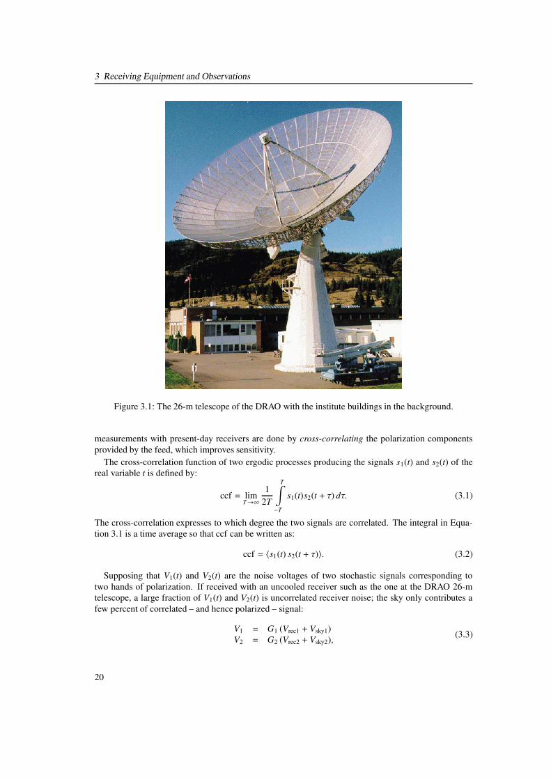
The 26-m telescope (Figure 3.1) was build in 1959. Since then, it has been frequently used for spec-troscopy of Galactic H and OH. It is a deep paraboloid ( f /D = 0.3, where f is the focal distance andD the diameter of the antenna) with an open-mesh surface. The telescope has a diameter of 25.6 mand is located at −119◦ 37.2′ longitude and +49◦ 19.2′ latitude. The antenna was originally intendedfor use at 1.4 GHz. At this frequency the aperture efficiency is 55% (10 Jy/K). The antenna surfaceallows observations at frequencies from about 400 MHz to about 8.4 GHz. At 6.6 GHz the apertureefficiency falls to 11%. Only few observations have been made towards the upper limit of the frequencyband. The receiver box is mounted on three support-struts which are arranged at an angle of 33.◦5 to theantenna boresight. Different primary focus boxes are available, hosting receivers operating at differentfrequencies.
The antenna is on a polar mount and can observe the sky between −34◦ and +90◦ declination. Surveyobservations were limited to declinations ≥ −27◦. The rms pointing accuracy is 0.8′ (Knee, 1997).Observations are usually scheduled several days in advance with the telescope left unattended.
3.1.2 Cross-Correlation of Radio Signals
In radio astronomical receivers operating in the Megahertz and lower Gigahertz range, a number ofmethods are used to stabilize the gain of the receiving system. Gain fluctuations of the amplifier chainand the 1/f-noise limit the detectability of weak radio signals. Aside from circuit designing the ampli-fiers as stable as possible, principles like the Dicke switch have been applied in the past. Polarimetric
19
3 Receiving Equipment and Observations
Figure 3.1: The 26-m telescope of the DRAO with the institute buildings in the background.
measurements with present-day receivers are done by cross-correlating the polarization componentsprovided by the feed, which improves sensitivity.
The cross-correlation function of two ergodic processes producing the signals s1(t) and s2(t) of thereal variable t is defined by:
ccf = limT→∞
12T
T∫
−T
s1(t)s2(t + τ) dτ. (3.1)
The cross-correlation expresses to which degree the two signals are correlated. The integral in Equa-tion 3.1 is a time average so that ccf can be written as:
ccf = 〈s1(t) s2(t + τ)〉. (3.2)
Supposing that V1(t) and V2(t) are the noise voltages of two stochastic signals corresponding totwo hands of polarization. If received with an uncooled receiver such as the one at the DRAO 26-mtelescope, a large fraction of V1(t) and V2(t) is uncorrelated receiver noise; the sky only contributes afew percent of correlated – and hence polarized – signal:
V1 = G1 (Vrec1 + Vsky1)V2 = G2 (Vrec2 + Vsky2), (3.3)
20
3.1 Hardware
��������������������������������������������������������������������������������������������������������������������������������������������������������������������������������������������������������������������������������������������������������������������������������������������������������������������������������������������������������������������������������������������������������������������������������������������������������������������������������������������������������������������������������������������������������������������������������������������������������������������������������������������������������������������������������������������������������������������������������������������������������������������������������������������������������������������������������������������������������������������������������������������������������������������������������������������������������������������������������������������������������������������������������������������������������������������������������������������������������������������������������������������������������������������������������������������������������������������������������������������������������������������������������������������������������������������������������������������������������������������������������������������������������������������������������������������������������������������������������������������������������������������������������������������������������������������������������������������������������������������������������������������������������������������������������������������������������������������������������������������������������������������������������������������������������������������
��������������������������������������������������������������������������������������������������������������������������������������������������������������������������������������������������������������������������������������������������������������������������������������������������������������������������������������������������������������������������������������������������������������������������������������������������������������������������������������������������������������������������������������������������������������������������������������������������������������������������������������������������������������������������������������������������������������������������������������������������������������������������������������������������������������������������������������������������������������������������������������������������������������������������������������������������������������������������������������������������������������������������������������������������������������������������������������������������������������������������������������������������������������������������������������������������������������������������������������������������������������������������������������������������������������������������������������������������������������������������������������������������������������������������������������������������������������������������������������������������������������������������������������������������������������������������������������������������������������������������������������������������������������������������������������������������������������������������������������������������������������������������������������������������������������������
���������������������������������������������������������������������������
���������������������������������������������������������������������������
COUPLER
LNACIRCULATOR
CIRCULATOR
LNA
"CAL"HYBRID
COUPLERCOUPLER
X−PORT
Y−PORT
SPLITTER
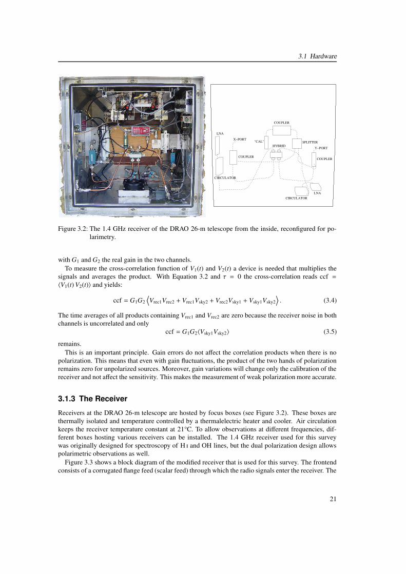
Figure 3.2: The 1.4 GHz receiver of the DRAO 26-m telescope from the inside, reconfigured for po-larimetry.
with G1 and G2 the real gain in the two channels.To measure the cross-correlation function of V1(t) and V2(t) a device is needed that multiplies the
signals and averages the product. With Equation 3.2 and τ = 0 the cross-correlation reads ccf =〈V1(t) V2(t)〉 and yields:
ccf = G1G2
⟨
Vrec1Vrec2 + Vrec1Vsky2 + Vrec2Vsky1 + Vsky1Vsky2
⟩
. (3.4)
The time averages of all products containing Vrec1 and Vrec2 are zero because the receiver noise in bothchannels is uncorrelated and only
ccf = G1G2〈Vsky1Vsky2〉 (3.5)
remains.This is an important principle. Gain errors do not affect the correlation products when there is no
polarization. This means that even with gain fluctuations, the product of the two hands of polarizationremains zero for unpolarized sources. Moreover, gain variations will change only the calibration of thereceiver and not affect the sensitivity. This makes the measurement of weak polarization more accurate.
3.1.3 The Receiver
Receivers at the DRAO 26-m telescope are hosted by focus boxes (see Figure 3.2). These boxes arethermally isolated and temperature controlled by a thermalelectric heater and cooler. Air circulationkeeps the receiver temperature constant at 21°C. To allow observations at different frequencies, dif-ferent boxes hosting various receivers can be installed. The 1.4 GHz receiver used for this surveywas originally designed for spectroscopy of H and OH lines, but the dual polarization design allowspolarimetric observations as well.
Figure 3.3 shows a block diagram of the modified receiver that is used for this survey. The frontendconsists of a corrugated flange feed (scalar feed) through which the radio signals enter the receiver. The
21

3 Receiving Equipment and Observations
DIRECTIONALCOUPLER
FRONTEND
FRONT−ENDCONTROL
CLK POLARIMETERCONTROL
CIRCULATOR
HYBRID
POLARIZER
HORN
LNA
RF FILTER
AMPLIFIER
MIXER
IF AMPLIFIER
IF BANDPASS
POLARIMETER
CA
L
CH
AN
NE
L A
CH
AN
NE
L B
LO
HYBR.
0/180
V/F
COUNTERS
PC
PCPCCOORDINATES
to ANTENNA
DATA
DATA
ATTENUATOR
ATTENUATOR
ATTENUATOR
X Y
o90
Figure 3.3: Block diagram of the 1410 MHz continuum receiver of the DRAO 26-m telescope afterreconfiguration for polarimetry.
22

3.1 Hardware
Table 3.1: Receiver and antenna specificationsTelescope coordinates −119◦ 37.2′, +49◦ 19.2′
Antenna diameter 25.6 mHPBW (effective) 36′
Aperture efficiency 55%Bandwidth (November 2002) 12 MHz (10 MHz)Poiting accuracy 0.8′
Intermediate frequency 150 MHzSystem temperature 161 KGain variations in 30 days . 4%Ambient temperature stability of the receiver ∼ 1°CPhase tracking across band ∼ 5◦
feed, which is scaled from a feed designed at the MPIfR, is followed by a piece of circular waveguideand a circular-to-square transition. A dual polarization coupler (DPC) splits the initial input signal intoits linear polarization components: Ex and Ey. A calibration signal is injected into the X- and Y-linesthrough directional couplers. The two signal lines are then cross-coupled by a quadrature hybrid, whichis followed by circulators. Two low-noise amplifiers (LNA) amplify the signals. The signals then gothrough bandpass filters centred at 1412.5 MHz with a 1 dB bandwidth of 35 MHz. The bandpass isfollowed by attenuation and more amplification. Subsequently, the signals are send into mixers whichturn the radio frequency (RF) signals into intermediate frequency (IF) signals centred at 150 MHz. Afterbeing once more attenuated, amplified, and bandpass filtered the IF-signals enter the polarimeter. Thepolarimeter has four output channels, which are connected to the data acquisition PC and continuouslyread-out.
Receiver Modifications
The original receiver does not have a quadrature hybrid and therefore provides linear polarizationcomponents. From the definition of the Stokes parameters (Equation 2.18) it can be seen that cross-correlating linear components does not yield measures for the polarization state of a linearly polarizedincoming wave. Although not used at the final receiver, the correlation products of linear componentsare now calculated for demonstration. Let Ex and Ey be the two analytic representations of a linearlypolarized signal corresponding to equation 2.2:
Ex = a1eiωt
Ey = a2eiωt.(3.6)
According to the receiver block diagram (Figure 3.3), the polarimeter performs two multiplications. Itcalculates the simple product of the two polarization components and the product in which one of thetwo components is phase shifted by 90◦:
ExE?y = a1a2
Ex,− π2E?
y = a1a2e−i π2 .(3.7)
The time-averages of these products are:
XY = Re(ExE?y ) = a1a2 =
a20
2 sin 2ϕ −→ Stokes UYX = Re(Ex,− π2 E?
y ) = a1a2 cos π2 = 0 −→ Stokes V,
(3.8)
23
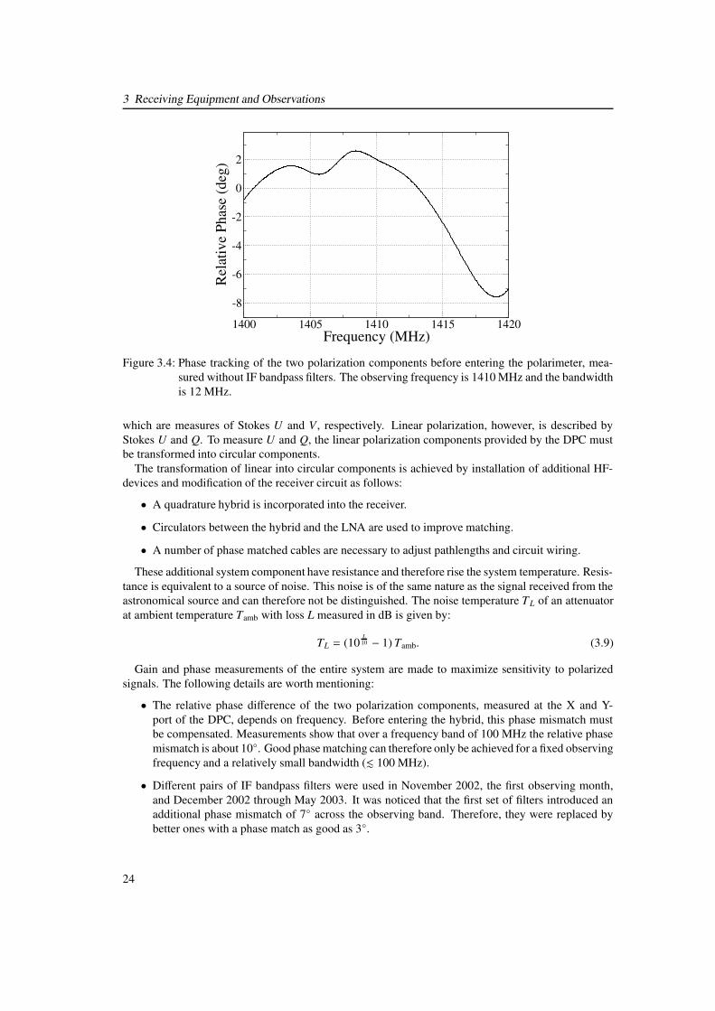
3 Receiving Equipment and Observations
1400 1405 1410 1415 1420Frequency (MHz)
-8
-6
-4
-2
0
2
Rel
ativ
e Ph
ase
(deg
)
Figure 3.4: Phase tracking of the two polarization components before entering the polarimeter, mea-sured without IF bandpass filters. The observing frequency is 1410 MHz and the bandwidthis 12 MHz.
which are measures of Stokes U and V, respectively. Linear polarization, however, is described byStokes U and Q. To measure U and Q, the linear polarization components provided by the DPC mustbe transformed into circular components.
The transformation of linear into circular components is achieved by installation of additional HF-devices and modification of the receiver circuit as follows:
• A quadrature hybrid is incorporated into the receiver.
• Circulators between the hybrid and the LNA are used to improve matching.
• A number of phase matched cables are necessary to adjust pathlengths and circuit wiring.
These additional system component have resistance and therefore rise the system temperature. Resis-tance is equivalent to a source of noise. This noise is of the same nature as the signal received from theastronomical source and can therefore not be distinguished. The noise temperature TL of an attenuatorat ambient temperature Tamb with loss L measured in dB is given by:
TL = (10L10 − 1) Tamb. (3.9)
Gain and phase measurements of the entire system are made to maximize sensitivity to polarizedsignals. The following details are worth mentioning:
• The relative phase difference of the two polarization components, measured at the X and Y-port of the DPC, depends on frequency. Before entering the hybrid, this phase mismatch mustbe compensated. Measurements show that over a frequency band of 100 MHz the relative phasemismatch is about 10◦. Good phase matching can therefore only be achieved for a fixed observingfrequency and a relatively small bandwidth (. 100 MHz).
• Different pairs of IF bandpass filters were used in November 2002, the first observing month,and December 2002 through May 2003. It was noticed that the first set of filters introduced anadditional phase mismatch of 7◦ across the observing band. Therefore, they were replaced bybetter ones with a phase match as good as 3◦.
24
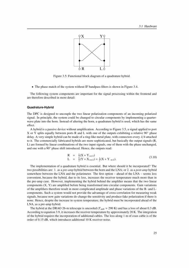
3.1 Hardware
LR
X Y
Figure 3.5: Functional block diagram of a quadrature hybrid.
• The phase match of the system without IF bandpass filters is shown in Figure 3.4.
The following system components are important for the signal processing within the frontend andare therefore described in more detail:
Quadrature-Hybrid
The DPC is designed to uncouple the two linear polarization components of an incoming polarizedsignal. In principle, the system could be changed to circular components by implementing a quarter-wave plate into the horn. Instead of altering the horn, a quadrature hybrid is used, which has the sameeffect.
A hybrid is a passive device without amplification. According to Figure 3.5, a signal applied to portX or Y splits equally between ports R and L with one of the outputs exhibiting a relative 90◦ phasedelay. A very simple hybrid can be made of a ring-like metal plate, with connectors every λ/4 attachedto it. The commercially fabricated hybrids are more sophisticated, but basically the output signals (R,L) are formed by linear combinations of the two input signals, one of them with the phase unchanged,and one with a 90◦ phase shift introduced. Hence, the outputs read:
R = 12 (X + Y+π/2)
L = 12 (Y + X+π/2) = 1
2 (X + Y−π/2). (3.10)
The implementation of a quadrature hybrid is essential. But where should it be incorporated? Thetwo possibilities are: 1. as a pre-amp hybrid between the horn and the LNA; or 2. as a post-amp hybridsomewhere between the LNA and the polarimeter. The first option – ahead of the LNA – seems lessconvenient, because the hybrid, due to its loss, increases the receiver temperature much more than inthe pre-amp case. However, implementing the hybrid behind the amplifier means that the two linearcomponents (X, Y) are amplified before being transformed into circular components. Gain variationsof the amplifiers therefore result in more complicated amplitude and phase variations of the R- and L-components. Such a system would not provide the advantage of cross-correlation for measuring weaksignals, because now gain variations do change the sensitivity and produce fake polarization if there isnone. Hence, despite the increase in system temperature, the hybrid must be incorporated ahead of theLNA, as a pre-amp hybrid.
The hybrid at the DRAO 26-m telescope is uncooled (Tamb ≈ 290 K) and has a loss of about 0.3 dB.According to equation 3.9, it increases the receiver temperature by approximately 20 K. The integrationof the hybrid requires the incorporation of additional cables. The loss along 1 m of coax cable is of theorder of 0.15 dB, which introduces additional 10 K receiver noise.
25
3 Receiving Equipment and Observations
Circulators
Circulators are added in to improve matching between the hybrid and the LNAs. This prevents backscat-tering of signals from the X- and Y-ports of the hybrid into the other, which would produce cross-talkand thus increase instrumental polarization.
A ferrite circulator or isolator is a device that allows RF to flow between two adjacent ports. Thisflow is restricted to one direction only. The transmission line is placed between ferrite material andmagnets. The magnetic field induced by the magnets allows RF to pass in one direction without beingattenuated, but not in the other direction.
The isolators used here have an insertion loss of about 0.25 dB and an isolation in the reverse di-rection of about −30 dB. According to Equation 3.9 the insertion loss rises the system temperature byabout 17 K.
Calibration Noise Source
A calibration signal is generated by a noise source, Noise/Com Inc Model NC3101E, generating asignal of constant amplitude. The “cal” is switched on every 24 s for a duration of 400 ms. The signalis split and injected through directional couplers and thus produces a correlated, polarized, signal at theX- and Y-ports of the hybrid.
Although the hybrid transforms a relative amplitude difference of Ex and Ey into a relative phasedifference between Er and El, and a relative phase difference between Ex and Ey into a relative am-plitude difference of Er and El, the gain and phase of the cal, measured at the X- and Y-port of thehybrid, do not have to be well matched. Important is that the cal produces signals in R and L that haveconstant amplitude and phase. This is then recorded as a constant reference signal in the RL and LRcross-correlations. The reference signals in RL and LR are later transformed into polarized intensityand polarization angle.
The directional couplers, through which the cal signal is injected, have an insertion loss of about0.2 dB on their main line. This adds additional 15 K to the receiver noise.
Low-Noise Amplifiers
Low-noise amplifiers are specifically designed to have a high gain and a comparatively low thermalnoise. The LNAs used here are two Berkshire (L-1.4-45HR) build in 1991. They have a quoted gain of57.0 dB, and 51.6 dB, respectively. The thermal noise of these amplifiers is about 30 K. These LNAsare based on HEMT transistors.
3.1.4 System Temperature
Because of their loss, the receiver components contribute thermal noise. This raises the effective noisetemperature of the receiver. The receiver temperature T rec is the sum of all noise contributions withinthe receiver. In case of the DRAO 26-m receiver, and in most other receivers used in radio astronomy,several amplification stages are combined serially as a cascade of amplifiers. It can be shown that thereceiver temperature of a cascaded system is:
Trec = T1 +1
G1T2 +
1G1G2
T3 + · · · +1
G1G2 . . .Gn−1Tn, (3.11)
(see e.g. Rohlfs & Wilson, 1996, for derivation) with Tn and Gn being the noise temperature and gainin the n-th amplification stage. Therefore, only the receiver components ahead of the first amplifier
26
3.1 Hardware
contribute significantly to the receiver temperature. In case of the receiver used for this survey, theseare the horn, DPC, couplers, hybrid, and circulators.
The system temperature is the sum of receiver temperature and all other noise contributions suchas antenna temperature. Antenna noise originates from the sky background, ohmic losses, and groundpickup or spillover from side lobes (atmospheric noise and the actual sky signal). Along with bandwidthand integration time, the system temperature determines the sensitivity of the receiver. The rms noisetemperature Trms of the system is defined by:
Trms =Cs Tsys√
B t, (3.12)
with bandwidth B and integration time t. The constant Cs depends on the type of receiver used for theobservations.
Adding the above listed noise contributions and allowing additional 60 K for ground radiation, atmo-spheric effects and other noise sources, the system temperature without sky emission results in about160 K. In case of total power observations, the constant Cs is unity (see various textbooks, e.g. Kraus,1966, p. 258). With a bandwidth of 12 MHz and an integration time of 60 s per pixel, the theoreticalrms due to receiver noise in total power is 6 mK.
The polarimetric measurements are done on correlated signals. The constant Cs is in case of acorrelation receiver 0.71 and the theoretical rms in the cross-correlated channels thus calculates to4 mK. These are theoretical values. The final errors in Stokes U and Q are greater for reasons discussedlater (Section 4.3).
3.1.5 Polarimeters
The only backend device utilized for this survey is a continuum polarimeter brought to DRAO fromEffelsberg. The S300-4 narrow band polarimeter is capable of performing the analog multiplication ofthree individual input channels of which only two are used here. The same type of polarimeter is usedon the Effelsberg 100-m telescope for narrow band polarimetry. Prior to shipping, a few modificationsof the polarimeter were made. All coax cables and lines were checked and replaced, if necessary. Theinternal multipliers were substituted by new ones with improved performance and the transformerswere replaced to stabilize power supply.
A multiplying polarimeter is a correlator that calculates products of the incoming signals. Usuallythese signals are the two polarization components of the received radio waves, ideally perfect linear orcircular. Different types of polarimeters are described now with an emphasis on analog polarimeters.
Analog Multiplying Polarimeter
Let Ex and Ey be the two analytic signals representing linear polarization components of a linearlypolarized radio wave (δ = 0) with amplitude A0 and position angle ϕ:
Ex = Axeiωt
Ey = Ayeiωt,(3.13)
withAx = A0 cosϕAy = A0 sinϕ. (3.14)
27

3 Receiving Equipment and Observations
In case of the DRAO 26-m-telescope receiver, linear components are transformed into circular by thehybrid:
Er = 0.5(
Ax eiωt + Ay ei(ωt− π2 ))
El = 0.5(
Ax ei(ωt− π2 ) + Ay eiωt
)
.(3.15)
These signals are fed into the polarimeter. Correlation of Er and El yields:
ErE?l = 1
4
(
Axeiωt + Ayei(ωt− π2 )) (
Axe−i(ωt− π2 ) + Aye−iωt
)
= 12 AxAy +
i4
(
A2x − A2
y
)
.(3.16)
The time-average of this product is Re (ErE?l ). With the amplitudes of the linear polarization compo-
nents Ax and Ay, this gives:
RL = Re (ErE?l ) =
12
AxAy =A2
0
4sin 2ϕ −→ Stokes U. (3.17)
According to the definition of the Stokes parameters, this product corresponds to Stokes U. Thispolarimeter channel is also called the sine-channel.
To achieve full information on the polarization state the polarimeter calculates a second product: theproduct of Er and Er, with Er phase-delayed by 90◦. The correlation then yields:
Er,− π2 E?l = 1
4
(
Axei(ωt− π2 ) + Ayei(ωt−π)
) (
Axe−i(ωt− π2 ) + Aye−iωt
)
= 14
(
A2x − A2
y
)
− i2 AxAy
(3.18)
with the time-average of this product:
LR = Re (Er,− π2 E?l ) =
14
(
A2x − A2
y
)
=A2
0
4cos 2ϕ −→ Stokes Q, (3.19)
which corresponds to Stokes Q. This polarimeter channel is also called the cosine-channel. The sine-and cosine-channels provide all information required to fully describe the polarization state of a linearlypolarized radio wave. In case of partial polarization Stokes I is also required.
In analog correlators the multiplication of the two input signals is done by multipliers. Such amultiplier takes advantage of the equation: (A + B)2 − (A − B)2 = 4AB. Hence, the product of A andB is determined by detecting the sum and difference of the two signals with square-law detectors, andsubsequently subtracting these signals. In practise, analog multipliers are subject to gain errors andnon-linearities. In particular the products contain quadratic terms in the form:
AB + αA2 + βB2, (3.20)
whereas α and β are usually small. Moreover, the products have DC offsets which are sensitive to theambient temperature. In case of the S300 polarimeter, the amplitude of fluctuations of the DC term isorders of magnitudes larger than signals caused by polarized radiation from the sky.
To handle quadratic terms and DC offsets, the correlation products are calculated twice: at first withthe relative phase between the two components unchanged and a second time with one of the two inputsignals phase shifted by 180◦. This causes the sign of the product AB to change, but not the sign of thequadratic terms and DC offsets. The phase shifter is switched periodically between zero and 180◦. Thepure correlation products can be recovered by taking the difference of the phase shifted and unshifted
28
3.1 Hardware
correlator outputs:RL = 0.5 (RL0 − RL180)LR = 0.5 (LR0 − LR180) . (3.21)
Digital Cross-Correlator
Digital cross-correlators are often used in synthesis telescopes but also some single-antenna telescopescross-correlate signals digitally (e.g. the Green-Bank Telescope). The inputs of such a correlator aredigitized samples of data from each antenna or each hand of polarization. The output of a correlatoris the cross-correlation function (ccf) of data received in a finite time interval, which is adapted to thebandwidth used for the observation. The digitized data within the time interval are called “lags”.
By Fourier transforming ccf consisting of N lags, a cross-power spectrum with N channels is ob-tained. As ccf is antisymmetric about τ = 0 (Equation 3.1) the Fourier transformation results in acomplex spectrum. If circular polarization components are correlated, the real and imaginary parts ofthe Fourier transformed ccf correspond to Stokes U and Q.
A correlator in which the correlation is followed by a Fourier transformation is called XF-correlator.It is called FX-correlation if the signals are first Fourier transformed and then multiplied.
Other Types of Polarimeters
In bolometric receivers the signals of the two hands of polarization are detected by square-law detectorsand thus phase information is not preserved. Stokes parameters are retrieved by adding and subtractingthe detected power levels in the following way:
I = RR + LLQ = RR − LL. (3.22)
Stokes U is measured by rotation of the plane of polarization with respect to the feed. In such polarime-ters, small quantities (U, Q) are derived by subtraction or addition of two large quantities (RR, LL). Thegain in the two channels must therefore be sufficiently stable, a challenging design goal. These types ofpolarimeters are sometimes used in bolometric receivers mapping the CMB polarization at frequenciesaround 100 GHz (e.g. Siringo et al., 2004; Tauber, 2004).
Another type of polarimeter is the adding polarimeter, which consists of a network of 90◦- and180◦-hybrids performing phase-correct additions. Instead of calculating products of Er and El such apolarimeter has the following outputs (see e.g. von Hoensbroech & Xilouris, 1997):
channel 1 =⟨
|Er|2⟩
=⟨
ErE?r
⟩
channel 2 =⟨
|El|2⟩
=⟨
ElE?l
⟩
.(3.23)
Total power I and Stokes V are derived from:
I = channel 1 + channel 2V = channel 2 − channel 1. (3.24)
Stokes U and Q are as follows:U = channel 4 − IQ = I − channel 3. (3.25)
Calibration is required to find scaling factors for total power I and the correlator output channels 3and 4. Again, the gain of the signals fed into such a polarimeter must be stable because Stokes U andQ are given by differences of large and small quantities.
29
3 Receiving Equipment and Observations
3.1.6 System Adjustments
The implementation of a hybrid requires the adjustment of relative gain and phase of the receiver chan-nels carrying the two hands of polarization. As the DPC provides linear polarization components ahybrid is used to form circular polarization hands out of linear. Within the hybrid this is done by phasedelaying and adding the linear components. But the hybrid as well as other receiver components intro-duce errors in terms of phase and gain mismatches between the two components. These mismatchesaffect the sensitivity of the receiving system to polarized signals and must be compensated by adjust-ment of cable length and integration of attenuators in the receiver circuit.
The following questions must be investigated to estimate the importance of system adjustments andrecognize systematic errors in the data :
• How do phase and gain mismatches of the linear polarization components (E x, Ey) in the pre-hybrid part affect the measurement of Stokes U and Q?
• How do gain and phase mismatches of the circular polarization components in the post-hybrid(Er, El) affect the cross-correlations (RL, LR)?
• The input signals have a bandwidth of 12 MHz. How do phase slopes across the observing bandalter the cross-correlations.
It now follows a discussion of these questions.
Phase- and Gain-Matching in the Pre-Hybrid Part
The adjustment of relative power levels and phases in the X and Y signal paths of the receiver, aheadof the hybrid, must be discussed. There are no active devices, such as amplifiers, in this part of thereceiver. All devices are passive and power level mismatches either reflect different polarization anglesof the incoming signal or are caused by different attenuation of the receiver components.
A phase mismatch may be caused, for example, by different cable lengths or the DPC itself. Tocalculate the effect of mismatches of the power levels and phases in the pre-hybrid part, the two complexgains gx = Gx eiεx and gy = Gy eiεy are introduced, with the two power gains Gx and Gy, and the pre-hybrid phase error ∆εxy = εx − εy. The linear polarization components are then expressed by:
Ex = Gx Ax ei(ωt+εx)
Ey = Gy Ay ei(ωt+εy).(3.26)
After passing through the hybrid the two linear polarization components are transformed into circular:
Er = 12
(
Gx Ax ei(ωt+εx) +Gy Ay ei(ωt+εy−π/2))
El = 12
(
Gx Ax ei(ωt+εx−π/2) +Gy Ay ei(ωt+εy))
.(3.27)
The real parts of the products measured with an analog polarimeter are:
RL = Re(ErE?l ) = 1
2GxGyAxAy cos∆εxy
LR = Re(Er,− π2 E?l ) = 1
4
(
G2xA2
x −G2y A2
y
)
.(3.28)
With the polarization angle ϕ, Ax = A0 cosϕ, and Ay = A0 sinϕ this becomes:
RL = 14 A2
0GxGy sin 2ϕ cos∆εxy
LR = 18 A2
0
(
G2x −G2
y +(
G2x +G2
y
)
cos 2ϕ) (3.29)
30
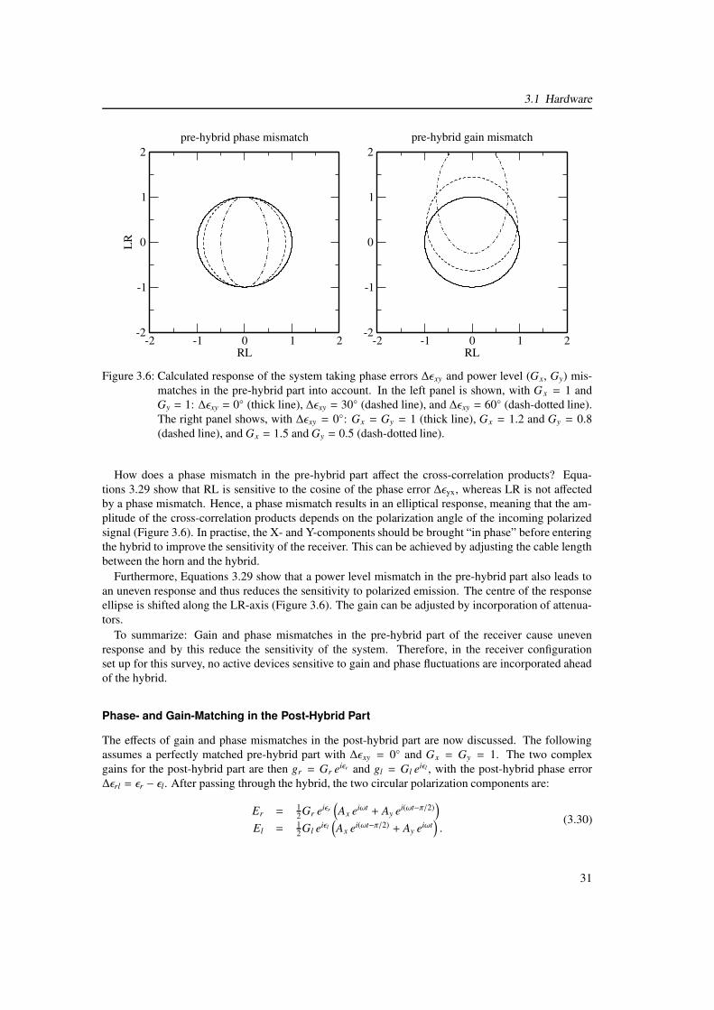
3.1 Hardware
-2 -1 0 1 2RL
-2
-1
0
1
2
LR
pre-hybrid phase mismatch
-2 -1 0 1 2RL
-2
-1
0
1
2pre-hybrid gain mismatch
Figure 3.6: Calculated response of the system taking phase errors ∆εxy and power level (Gx, Gy) mis-matches in the pre-hybrid part into account. In the left panel is shown, with G x = 1 andGy = 1: ∆εxy = 0◦ (thick line), ∆εxy = 30◦ (dashed line), and ∆εxy = 60◦ (dash-dotted line).The right panel shows, with ∆εxy = 0◦: Gx = Gy = 1 (thick line), Gx = 1.2 and Gy = 0.8(dashed line), and Gx = 1.5 and Gy = 0.5 (dash-dotted line).
How does a phase mismatch in the pre-hybrid part affect the cross-correlation products? Equa-tions 3.29 show that RL is sensitive to the cosine of the phase error ∆εyx, whereas LR is not affectedby a phase mismatch. Hence, a phase mismatch results in an elliptical response, meaning that the am-plitude of the cross-correlation products depends on the polarization angle of the incoming polarizedsignal (Figure 3.6). In practise, the X- and Y-components should be brought “in phase” before enteringthe hybrid to improve the sensitivity of the receiver. This can be achieved by adjusting the cable lengthbetween the horn and the hybrid.
Furthermore, Equations 3.29 show that a power level mismatch in the pre-hybrid part also leads toan uneven response and thus reduces the sensitivity to polarized emission. The centre of the responseellipse is shifted along the LR-axis (Figure 3.6). The gain can be adjusted by incorporation of attenua-tors.
To summarize: Gain and phase mismatches in the pre-hybrid part of the receiver cause unevenresponse and by this reduce the sensitivity of the system. Therefore, in the receiver configurationset up for this survey, no active devices sensitive to gain and phase fluctuations are incorporated aheadof the hybrid.
Phase- and Gain-Matching in the Post-Hybrid Part
The effects of gain and phase mismatches in the post-hybrid part are now discussed. The followingassumes a perfectly matched pre-hybrid part with ∆εxy = 0◦ and Gx = Gy = 1. The two complexgains for the post-hybrid part are then gr = Gr eiεr and gl = Gl eiεl , with the post-hybrid phase error∆εrl = εr − εl. After passing through the hybrid, the two circular polarization components are:
Er = 12Gr eiεr
(
Ax eiωt + Ay ei(ωt−π/2))
El =12Gl eiεl
(
Ax ei(ωt−π/2) + Ay eiωt)
.(3.30)
31
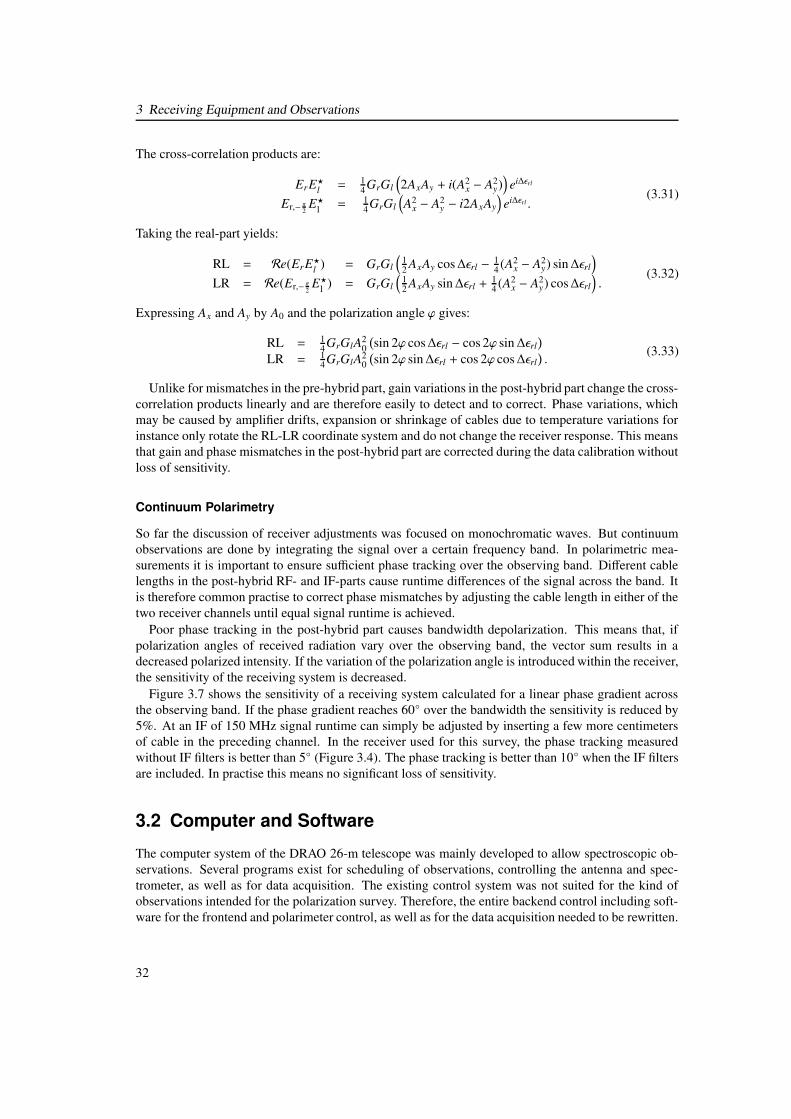
3 Receiving Equipment and Observations
The cross-correlation products are:
ErE?l = 1
4GrGl
(
2AxAy + i(A2x − A2
y))
ei∆εrl
Er,− π2E?
l = 14GrGl
(
A2x − A2
y − i2AxAy
)
ei∆εrl .(3.31)
Taking the real-part yields:
RL = Re(ErE?l ) = GrGl
(
12 AxAy cos∆εrl − 1
4 (A2x − A2
y) sin∆εrl
)
LR = Re(Er,− π2 E?l ) = GrGl
(
12 AxAy sin∆εrl +
14 (A2
x − A2y) cos∆εrl
)
.(3.32)
Expressing Ax and Ay by A0 and the polarization angle ϕ gives:
RL = 14GrGlA2
0(
sin 2ϕ cos∆εrl − cos 2ϕ sin∆εrl)
LR = 14GrGlA2
0(
sin 2ϕ sin∆εrl + cos 2ϕ cos∆εrl)
.(3.33)
Unlike for mismatches in the pre-hybrid part, gain variations in the post-hybrid part change the cross-correlation products linearly and are therefore easily to detect and to correct. Phase variations, whichmay be caused by amplifier drifts, expansion or shrinkage of cables due to temperature variations forinstance only rotate the RL-LR coordinate system and do not change the receiver response. This meansthat gain and phase mismatches in the post-hybrid part are corrected during the data calibration withoutloss of sensitivity.
Continuum Polarimetry
So far the discussion of receiver adjustments was focused on monochromatic waves. But continuumobservations are done by integrating the signal over a certain frequency band. In polarimetric mea-surements it is important to ensure sufficient phase tracking over the observing band. Different cablelengths in the post-hybrid RF- and IF-parts cause runtime differences of the signal across the band. Itis therefore common practise to correct phase mismatches by adjusting the cable length in either of thetwo receiver channels until equal signal runtime is achieved.
Poor phase tracking in the post-hybrid part causes bandwidth depolarization. This means that, ifpolarization angles of received radiation vary over the observing band, the vector sum results in adecreased polarized intensity. If the variation of the polarization angle is introduced within the receiver,the sensitivity of the receiving system is decreased.
Figure 3.7 shows the sensitivity of a receiving system calculated for a linear phase gradient acrossthe observing band. If the phase gradient reaches 60◦ over the bandwidth the sensitivity is reduced by5%. At an IF of 150 MHz signal runtime can simply be adjusted by inserting a few more centimetersof cable in the preceding channel. In the receiver used for this survey, the phase tracking measuredwithout IF filters is better than 5◦ (Figure 3.4). The phase tracking is better than 10◦ when the IF filtersare included. In practise this means no significant loss of sensitivity.
3.2 Computer and Software
The computer system of the DRAO 26-m telescope was mainly developed to allow spectroscopic ob-servations. Several programs exist for scheduling of observations, controlling the antenna and spec-trometer, as well as for data acquisition. The existing control system was not suited for the kind ofobservations intended for the polarization survey. Therefore, the entire backend control including soft-ware for the frontend and polarimeter control, as well as for the data acquisition needed to be rewritten.
32
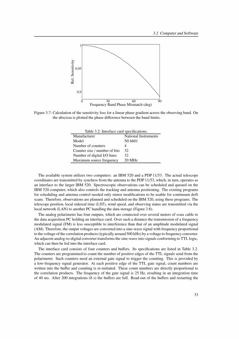
3.2 Computer and Software
0 30 60 90Frequency Band Phase Mismatch (deg)
0,9
0,95
1
Rel
. Sen
sitiv
ity
Figure 3.7: Calculation of the sensitivity loss for a linear phase gradient across the observing band. Onthe abscissa is plotted the phase difference between the band limits.
Table 3.2: Interface card specifications.Manufacturer National InstrumentsModel NI 6601Number of counters 4Counter size / number of bits 32Number of digital I/O lines 32Maximum source frequency 20 MHz
The available system utilizes two computers: an IBM 520 and a PDP 11/53. The actual telescopecoordinates are transmitted by synchros from the antenna to the PDP 11/53, which, in turn, operates asan interface to the larger IBM 520. Spectroscopic observations can be scheduled and queued on theIBM 520 computer, which also controls the tracking and antenna positioning. The existing programsfor scheduling and antenna control needed only minor modifications to be usable for continuum driftscans. Therefore, observations are planned and scheduled on the IBM 520, using these programs. Thetelescope position, local sidereal time (LST), wind speed, and observing status are transmitted via thelocal network (LAN) to another PC handling the data storage (Figure 3.8).
The analog polarimeter has four outputs, which are connected over several meters of coax cable tothe data acquisition PC holding an interface card. Over such a distance the transmission of a frequencymodulated signal (FM) is less susceptible to interference than that of an amplitude modulated signal(AM). Therefore, the output voltages are converted into a sine-wave signal with frequency proportionalto the voltage of the correlation products (typically around 500 kHz) by a voltage to frequency converter.An adjacent analog-to-digital converter transforms the sine-wave into signals conforming to TTL logic,which can then be fed into the interface card.
The interface card consists of four counters and buffers. Its specifications are listed in Table 3.2.The counters are programmed to count the number of positive edges of the TTL signals send from thepolarimeter. Such counters need an external gate signal to trigger the counting. This is provided bya low-frequency signal generator. At each positive edge of the TTL gate signal, count numbers arewritten into the buffer and counting is re-initiated. These count numbers are directly proportional tothe correlation products. The frequency of the gate signal is 25 Hz, resulting in an integration timeof 40 ms. After 200 integrations (8 s) the buffers are full. Read-out of the buffers and restarting the
33

3 Receiving Equipment and Observations
Data AcquisitionPC
AdditionalInformation
ObservingSchedule
WaterfalDisplay
ProgramData Storage
LAN Flag
s
Ch−
4C
h−3
Ch−
2C
h−1
Stat
usW
ind
Coo
rd.
LST
TT
LTT
L
"cal"
Polarimeter
IBM 520
PDP 11/53
Data Distribution Program (Mom)
ASCII−File
Figure 3.8: Flow diagram of the data stream as explained in the text.
counters requires about 400 ms. This results in cycles of roughly 8.4 s during which 4× 200 packets ofintegrations are gathered and transmitted to the data storage PC.
The interface card is also equipped with digital I/O lines. These lines are used to control the noisesource of the receiver and the internal 0/180◦-phase shifter of the polarimeter. During intervals of 200integrations (∼ 8 s), the phase shifter is set to 0◦ during the first half of the cycle (∼ 4 s) and 180◦ duringthe second half (∼ 4 s), resulting in 100 integrations at each phase. The noise source is switched everythird cycle.
The data reduction is done later on separate PCs, involving different stages of data reading, pro-cessing, flagging and gridding. The data acquisition and most of the reduction and calibration toolsdescribed in the following sections are written in glish, a scripting language within the AIPS++ (Mc-Mullin et al., 2004) environment. It was not possible to take advantage of the TOOLBOX package usedat the Effelsberg 100-m telescope because of lacking detailed documentation.
3.2.1 Telescope Scheduling Software
The program used for scheduling of survey observations drives and holds the telescope at given co-ordinates. The telescope control software was not intended for drift scanning and tries to correct thetelescope position after 60 minutes of observing. Therefore, drift scans are observed as sub scans with57 minute lengths each.
34

3.3 Instrumental Errors – Time-Invariable
Another problem with telescope positioning was encountered at declinations larger than 85◦, proba-bly because of limitations of the pointing model. Here, the telescope cannot be controlled by softwarebut must be positioned manually.
3.2.2 Data Acquisition Software
On the data storage PC, data streams carrying information about the current telescope status, ongoingobservations, telescope position, LST, and wind speed are continuously read-out by the data distributionprogram (Figure 3.9, top). This program merges the data on arrival and forwards them to the datastorage program (Figure 3.9, bottom) in an appropriate format. In addition, the data are displayed forchecking purposes on the “Waterfall Display” (Figure 3.10).
The data distribution program also corrects the telescope position sent from the IBM 520, becausethe telescope position is provided in equatorial coordinates in the current epoch. These coordinatesmust be transformed to J2000 coordinates. Additionally, the pointing model must be subtracted fromthese coordinates as the IBM 520 automatically applies the pointing correction.
Telescope-use prevented access to the system before July 2002. The data acquisition software, whichtherefore needed to be written prior to the completion of the hardware, had to be as flexible as possible.It was also not fully decided which observing modes will be available: whether, e.g. the telescope willbe capable of observing maps, etc.
3.2.3 Data Reduction Program
The raw data must be processed before their quality can be examined. This is done by the data reductionprogram (DRP, Figure 3.11). This program reads the raw data, which are stored on disk in form ofASCII-files, and performs the following processing steps:
1. Removal of spikes and interference as explained in Section 4.1.1.
2. Separation of the different states of the internal phase switch and calibration signal, taking circuittimes into account.
3. Calculation of the cross-correlation values by computing the difference of the signals of channel3 and 4 at phase zero and 180◦ of the polarimeter (Equation 3.21).
4. Averaging packets of data of 4 × 200 integrations.
Any further reduction steps such as calibration, gridding, and interpolation will be described inChapter 4. These data reduction steps are implemented by glish-scripts rather than graphical programs.
3.3 Instrumental Errors – Time-Invariable
The discussion in Section 3.1.6 demonstrated the point of relative gain and phase adjustments in thereceiving system to maximize sensitivity and circularity of the response. Apart from errors due to gainand phase mismatches, the system components themselves may introduce errors such as cross-couplingor non-circular responses. These errors modify the initial Stokes parameters of the source and are mostgenerally described by a 4× 4 matrix, the Müller matrix. In this section the formalism used to describethese errors will be explained, roughly following Heiles et al. (2001) and Heiles (2002).
35
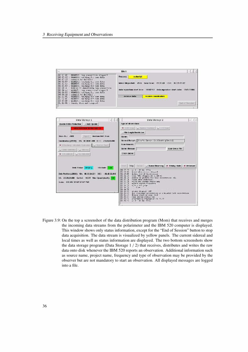
3 Receiving Equipment and Observations
Figure 3.9: On the top a screenshot of the data distribution program (Mom) that receives and mergesthe incoming data streams from the polarimeter and the IBM 520 computer is displayed.This window shows only status information, except for the “End of Session” button to stopdata acquisition. The data stream is visualized by yellow panels. The current sidereal andlocal times as well as status information are displayed. The two bottom screenshots showthe data storage program (Data Storage 1 / 2) that receives, distributes and writes the rawdata onto disk whenever the IBM 520 reports an observation. Additional information suchas source name, project name, frequency and type of observation may be provided by theobserver but are not mandatory to start an observation. All displayed messages are loggedinto a file.
36
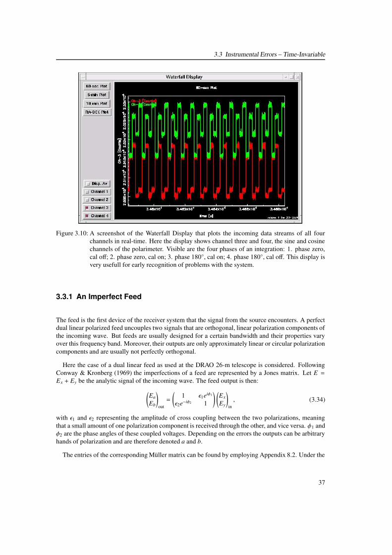
3.3 Instrumental Errors – Time-Invariable
Figure 3.10: A screenshot of the Waterfall Display that plots the incoming data streams of all fourchannels in real-time. Here the display shows channel three and four, the sine and cosinechannels of the polarimeter. Visible are the four phases of an integration: 1. phase zero,cal off; 2. phase zero, cal on; 3. phase 180◦, cal on; 4. phase 180◦, cal off. This display isvery usefull for early recognition of problems with the system.
3.3.1 An Imperfect Feed
The feed is the first device of the receiver system that the signal from the source encounters. A perfectdual linear polarized feed uncouples two signals that are orthogonal, linear polarization components ofthe incoming wave. But feeds are usually designed for a certain bandwidth and their properties varyover this frequency band. Moreover, their outputs are only approximately linear or circular polarizationcomponents and are usually not perfectly orthogonal.
Here the case of a dual linear feed as used at the DRAO 26-m telescope is considered. FollowingConway & Kronberg (1969) the imperfections of a feed are represented by a Jones matrix. Let E =Ex + Ey be the analytic signal of the incoming wave. The feed output is then:
(
Ea
Eb
)
out=
(
1 ε1eiφ1
ε2e−iφ2 1
) (
Ex
Ey
)
in, (3.34)
with ε1 and ε2 representing the amplitude of cross coupling between the two polarizations, meaningthat a small amount of one polarization component is received through the other, and vice versa. φ1 andφ2 are the phase angles of these coupled voltages. Depending on the errors the outputs can be arbitraryhands of polarization and are therefore denoted a and b.
The entries of the corresponding Müller matrix can be found by employing Appendix 8.2. Under the
37
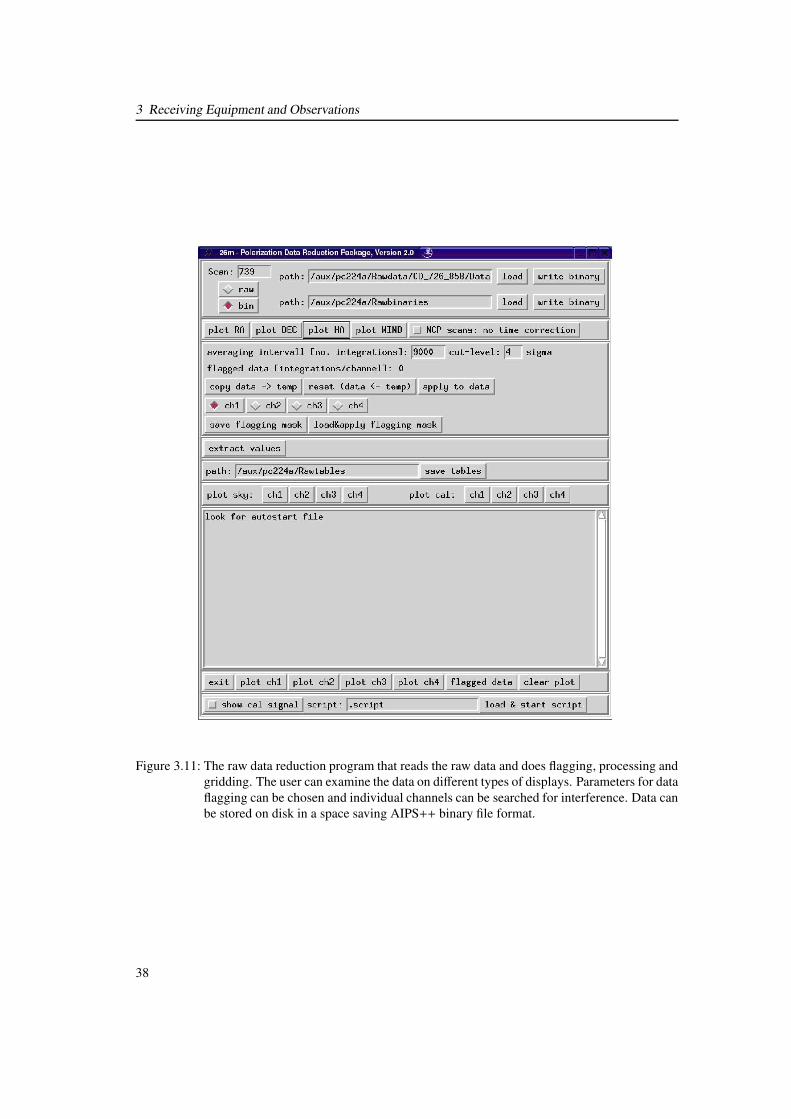
3 Receiving Equipment and Observations
Figure 3.11: The raw data reduction program that reads the raw data and does flagging, processing andgridding. The user can examine the data on different types of displays. Parameters for dataflagging can be chosen and individual channels can be searched for interference. Data canbe stored on disk in a space saving AIPS++ binary file format.
38
3.3 Instrumental Errors – Time-Invariable
assumption that ε1 ≈ ε2 ≈ 0 the transformation of the original signal by the feed reads:
S 1S 2
S 3S 4
out
=Mfeed
IQUV
in
with Mfeed =
1 0 αf βf0 1 γf δf
αf −γf 1 0βf −δf 0 1
, (3.35)
andαf = ε1 cos φ1 + ε2 cosφ2
βf = ε1 sin φ1 + ε2 sin φ2γf = ε1 cos φ1 − ε2 cosφ2
δf = ε1 sin φ1 − ε2 sin φ2.
(3.36)
The imperfections of a feed are described by four independent parameters to good approximation.
3.3.2 The Quadrature Hybrid
The quadrature hybrid forms the sum of two input signals while phase shifting one of the inputs. In aperfect hybrid the signal powers are split equally and the phase shift is exactly 90◦. Again, hybrids aredesigned for a specific frequency range and the perfect hybrid is achieved only to a certain degree.
In general, a hybrid can be described by the following Jones matrix:
(
Ea
Eb
)
out=
√0.5 gyaeiφya
gxbeiφxb√
0.5
(
Ex
Ey
)
in, (3.37)
with gya = gxb =√
0.5 and φya = φxb = −90◦ for a perfect hybrid in which case Ea and Eb were rightand left handed polarization components. Depending on the hybrid they do not have to be perfectlycircular so they are denoted a and b.
Under the assumption that gya ≈ gxb ≈√
0.5, the corresponding Müller matrix for the hybrid is:
S 1S 2
S 3
S 4
out
=Mhybrid
IQUV
in
with Mhybrid =
1 0 αh βh0 0 γh δh
αh −γh 1 0βh −δh 0 0
, (3.38)
withαh =
√0.5
(
gya cos φya + gxb cos φxb
)
βh =√
0.5(
−gya sin φya + gxb sin φxb
)
γh =√
0.5(
gya cos φya − gxb cos φxb
)
δh =√
0.5(
−gya sin φya − gxb sin φxb
)
.
(3.39)
In case of a perfect hybrid the Stokes parameters S 1, S 2, S 3, and S 4 can be associated with Stokes I,−V, U, and −Q. Hence, the perfect hybrid – or a quarter-wave plate within the horn – only changes theorder of Stokes parameters in the output vector.
3.3.3 System Gain
After being converted into approximate circular polarization components, the signals go through dif-ferent amplifier chains. These chains have complex gains, causing different amplification and phasedelays. The system gain therefore represents the time-independent signal deformation of the receiving
39
3 Receiving Equipment and Observations
system. Unlike electronic gain, the system gain describes steady properties of the system devices andmay only change by modification of the receiving system. The Jones matrix for the system gain is:
(
Ex
Ey
)
out=
(
gxeiψx 00 gyeiψy
) (
Ex
Ey
)
in, (3.40)
with the voltage gains gx and gy and the phase delays ψx and ψy. The corresponding Müller matrix forthe system gain is:
S 1
S 2S 3
S 4
out
=Mamp
IQUV
in
, (3.41)
with
Mamp =
12
(
g2x + g2
y
)
12
(
g2x − g2
y
)
0 012
(
g2x − g2
y
)
12
(
g2x + g2
y
)
0 00 0 gxgy cos∆ψ −gxgy sin∆ψ0 0 gxgy sin∆ψ gxgy cos∆ψ
, (3.42)
here ∆ψ = ψx − ψy can be considered a phase mismatch in the post-hybrid part which results in a 2 × 2sub rotation-matrix in the Müller matrix.
3.3.4 The System Müller Matrix
In principle one can set up an individual Müller matrix for each component of the receiving system.The product of all matrices results in a matrix describing the entire system. The order in which thesematrices must be applied corresponds to the signal path through the receiving system. Taking the abovementioned matrices as examples the transformation of the incoming signal is described by:
S 1S 2
S 3
S 4
out
=MampMhybridMfeedMPA
IQUV
in
. (3.43)
In general, the matrixMPA represents the rotation of the sky relative to the receiver coordinates and isa simple rotation matrix affecting only Stokes Uin and Qin. This must only be taken into account forazimuthal mounted telescopes. In case of the DRAO 26-m telescope it is the unit matrix due to theequatorial mounting.
The system Müller matrix has 7 free parameters and an irrelevant phase. Algebraic multiplication ofthe individual matrices results in a far too complicated system matrix. This would be of no use for thecalibration of the 26-m Survey, therefore the following form is used.
Assuming a uniform (perfect) system gain, which can be achieved by a pre-calibration, matrix mul-tiplication gives the system Jones matrix taking only the feed and hybrid into account:
Jsys =
[√0.5 + gyaε2ei(φya−φ2)
] [√0.5ε1eiφ1 + gyaeiφya
]
[
gxbeiφxb +√
0.5ε2e−iφ2] [√
0.5 + gxbε1ei(φxb+φ1)]
, (3.44)
40
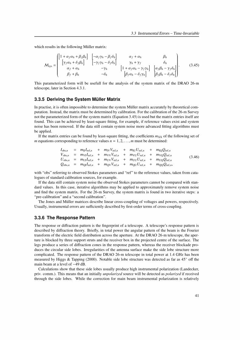
3.3 Instrumental Errors – Time-Invariable
which results in the following Müller matrix:
Msys =
[
1 + α fαh + β f βh
] [
−α f γh − β f δh
]
α f + αh βh[
γ fαh + δ fβh
] [
−γ fγh − δ f δh
]
γh + γ f δh
α f + αh −γh
[
1 + α fαh − γ f γh
] [
α fβh − γ f δh
]
β f + βh −δh
[
β fαh − δ fγh
] [
β f βh − δ f δh
]
. (3.45)
This parameterized form will be usefull for the analysis of the system matrix of the DRAO 26-mtelescope, later in Section 4.3.1.
3.3.5 Deriving the System Müller Matrix
In practise, it is often impossible to determine the system Müller matrix accurately by theoretical com-putation. Instead, the matrix must be determined by calibration. For the calibration of the 26-m Surveynot the parameterized form of the system matrix (Equation 3.45) is used but the matrix entries itself arefound. This can be achieved by least-square fitting, for example, if reference values exist and systemnoise has been removed. If the data still contain system noise more advanced fitting algorithms mustbe applied.
If the matrix entries can be found by least-square fitting, the coefficients mXX of the following set ofm equations corresponding to reference values n = 1, 2, . . . ,m must be determined:
Iobs,n = mIIIref,n + mIVVref,n + mIUUref,n + mIQQref,n
Vobs,n = mVIIref,n + mVVVref,n + mVUUref,n + mVQQref,nUobs,n = mUIIref,n + mUVVref,n + mUUUref,n + mUQQref,n
Qobs,n = mQIIref,n + mQVVref,n + mQUUref,n + mQQQref,n,
(3.46)
with “obs” referring to observed Stokes parameters and “ref” to the reference values, taken from cata-logues of standard calibration sources, for example.
If the data still contain system noise the observed Stokes parameters cannot be compared with stan-dard values. In this case, iterative algorithms may be applied to approximately remove system noiseand find the system matrix. For the 26-m Survey, the system matrix is found in two iterative steps: a“pre-calibration” and a “second calibration”.
The Jones and Müller matrices describe linear cross-coupling of voltages and powers, respectively.Usually, instrumental errors are sufficiently described by first-order terms of cross-coupling.
3.3.6 The Response Pattern
The response or diffraction pattern is the fingerprint of a telescope. A telescope’s response pattern isdescribed by diffraction theory. Briefly, in total power the angular pattern of the beam is the Fouriertransform of the electric field distribution across the aperture. At the DRAO 26-m telescope, the aper-ture is blocked by three support struts and the receiver box in the projected centre of the surface. Thelegs produce a series of diffraction cones in the response pattern, whereas the receiver blockade pro-duces the circular side lobes. Irregularities of the antenna surface make the side lobe structure morecomplicated. The response pattern of the DRAO 26-m telescope in total power at 1.4 GHz has beenmeasured by Higgs & Tapping (2000). Notable side lobe structure was detected as far as 45◦ off themain beam at a level of −49 dB.
Calculations show that these side lobes usually produce high instrumental polarization (Landecker,priv. comm.). This means that an initially unpolarized source will be detected as polarized if receivedthrough the side lobes. While the correction for main beam instrumental polarization is relatively
41
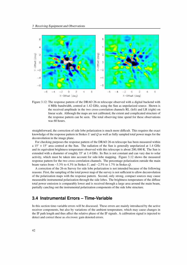
3 Receiving Equipment and Observations
Figure 3.12: The response pattern of the DRAO 26-m telescope observed with a digital backend with4 MHz bandwidth, centred at 1.42 GHz, using the Sun as unpolarized source. Shown isthe received amplitude in the two cross-correlation channels RL (left) and LR (right) onlinear scale. Although the maps are not calibrated, the extent and complicated structure ofthe response pattern can be seen. The total observing time spend for these observationswas 60 hours.
straightforward, the correction of side lobe polarization is much more difficult. This requires the exactknowledge of the response pattern in Stokes U and Q as well as fully sampled total power maps for thedeconvolution in the image plane.
For checking purposes the response pattern of the DRAO 26-m telescope has been measured withina 15◦ × 15◦ area centred at the Sun. The radiation of the Sun is generally unpolarized at 1.4 GHzand its equivalent brightness temperature observed with this telescope is about 200, 000 K. The Sun isextended with a diameter of roughly 35′ at 1.4 GHz. Its flux is not constant and can vary due to solaractivity, which must be taken into account for side-lobe mapping. Figure 3.12 shows the measuredresponse pattern for the two cross-correlation channels. The percentage polarization outside the mainbeam varies from −3.3% to 4.3% in Stokes U, and −2.5% to 1.7% in Stokes Q.
A correction of the 26-m Survey for side lobe polarization is not intended because of the followingreasons: First, the sampling of the total power map of the survey is not sufficient to allow deconvolutionof the polarization maps with the response pattern. Second, only strong, compact sources may causemeasurable instrumental polarization through the side lobes. The brightness temperature of the diffusetotal power emission is comparably lower and is received through a large area around the main beam,partially cancling out the instrumental polarization components of the side lobe structure.
3.4 Instrumental Errors – Time-Variable
In this section time-variable errors will be discussed. These errors are mainly introduced by the activereceiver components, but also by variations of the ambient temperature, which may cause changes inthe IF path length and thus affect the relative phase of the IF signals. A calibration signal is injected todetect and correct these as electronic gain denoted errors.
42
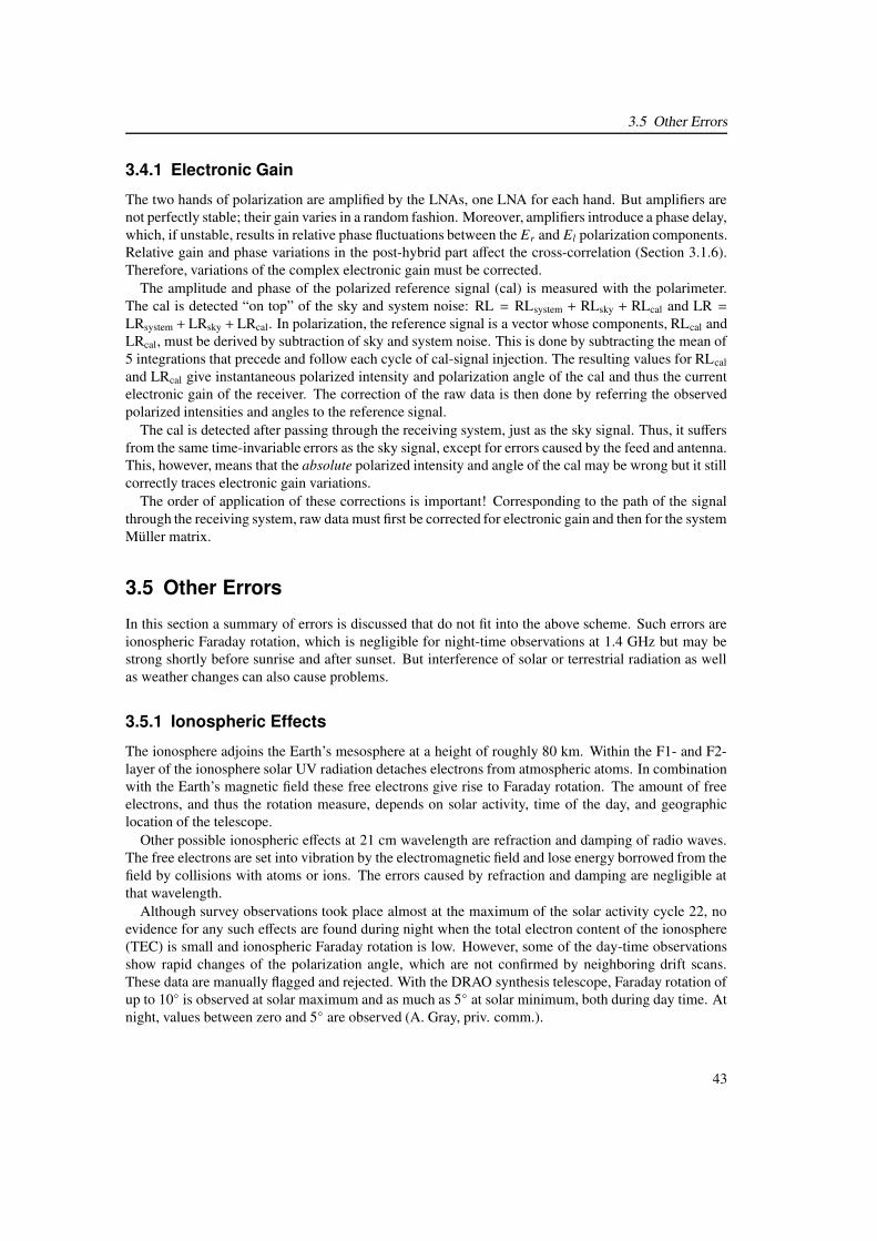
3.5 Other Errors
3.4.1 Electronic Gain
The two hands of polarization are amplified by the LNAs, one LNA for each hand. But amplifiers arenot perfectly stable; their gain varies in a random fashion. Moreover, amplifiers introduce a phase delay,which, if unstable, results in relative phase fluctuations between the Er and El polarization components.Relative gain and phase variations in the post-hybrid part affect the cross-correlation (Section 3.1.6).Therefore, variations of the complex electronic gain must be corrected.
The amplitude and phase of the polarized reference signal (cal) is measured with the polarimeter.The cal is detected “on top” of the sky and system noise: RL = RLsystem + RLsky + RLcal and LR =LRsystem + LRsky + LRcal. In polarization, the reference signal is a vector whose components, RLcal andLRcal, must be derived by subtraction of sky and system noise. This is done by subtracting the mean of5 integrations that precede and follow each cycle of cal-signal injection. The resulting values for RLcal
and LRcal give instantaneous polarized intensity and polarization angle of the cal and thus the currentelectronic gain of the receiver. The correction of the raw data is then done by referring the observedpolarized intensities and angles to the reference signal.
The cal is detected after passing through the receiving system, just as the sky signal. Thus, it suffersfrom the same time-invariable errors as the sky signal, except for errors caused by the feed and antenna.This, however, means that the absolute polarized intensity and angle of the cal may be wrong but it stillcorrectly traces electronic gain variations.
The order of application of these corrections is important! Corresponding to the path of the signalthrough the receiving system, raw data must first be corrected for electronic gain and then for the systemMüller matrix.
3.5 Other Errors
In this section a summary of errors is discussed that do not fit into the above scheme. Such errors areionospheric Faraday rotation, which is negligible for night-time observations at 1.4 GHz but may bestrong shortly before sunrise and after sunset. But interference of solar or terrestrial radiation as wellas weather changes can also cause problems.
3.5.1 Ionospheric Effects
The ionosphere adjoins the Earth’s mesosphere at a height of roughly 80 km. Within the F1- and F2-layer of the ionosphere solar UV radiation detaches electrons from atmospheric atoms. In combinationwith the Earth’s magnetic field these free electrons give rise to Faraday rotation. The amount of freeelectrons, and thus the rotation measure, depends on solar activity, time of the day, and geographiclocation of the telescope.
Other possible ionospheric effects at 21 cm wavelength are refraction and damping of radio waves.The free electrons are set into vibration by the electromagnetic field and lose energy borrowed from thefield by collisions with atoms or ions. The errors caused by refraction and damping are negligible atthat wavelength.
Although survey observations took place almost at the maximum of the solar activity cycle 22, noevidence for any such effects are found during night when the total electron content of the ionosphere(TEC) is small and ionospheric Faraday rotation is low. However, some of the day-time observationsshow rapid changes of the polarization angle, which are not confirmed by neighboring drift scans.These data are manually flagged and rejected. With the DRAO synthesis telescope, Faraday rotation ofup to 10◦ is observed at solar maximum and as much as 5◦ at solar minimum, both during day time. Atnight, values between zero and 5◦ are observed (A. Gray, priv. comm.).
43
3 Receiving Equipment and Observations
Figure 3.13: Example map of the TEC from February 21, 2005 demonstrating the distributionof electrons in the ionosphere during night in Canada. The map is taken fromhttp://iono.jpl.nasa.gov/.
Presently, the capabilities for a prediction and correction of these effects are limited. Althoughionospheric effects are negligible in the survey data, two approaches for the correction of ionosphericFaraday rotation are mentioned here. These are the theoretical modelling of the ionosphere and thedirect measurement of the electron content.
Campbell (1999) has suggested a prediction of ionospheric Faraday rotation by using the Parameter-ized Ionospheric Model (PIM). The PIM is a theoretical model of the global ionospheric climatology,developed at USAF Phillips Laboratory. Originally, PIM was intended to calculate the TEC of theatmosphere. A variant of PIM, initially motivated for application to VLBI astrometry (PIMVLBI),includes routines to calculate B‖ and B⊥ of the Earth’s magnetic field for a given line-of-sight. Theusefullness of PIM and PIMVLBI for the correction of polarization data is rather limited because it is astatic model that is not intended for generating time-series of ionospheric conditions. Moreover, it oftenfails to predict the right trend late in the day. At DRAO, another model is under development based onChapman layers using the solar flux at 10.7 cm as input. Initial versions seem promising, predictingtrends correctly where PIM fails (A. Gray, K. Tapping, priv. comm.).
The other approach requires a GPS (Global Positioning System) receiver installed at the telescopesite. With such a receiver the TEC can be monitored for the local site. By measurement of the timedelay of the GPS signals, the ionospheric-induced delay and hence the TEC along the line-of-sight toeach visible satellite can be determined. In conjunction with an ionospheric model this method makesan accurate correction possible. Tests at the VLA have shown that the accuracy is sufficient to correctfor Faraday effects to <∼ 2◦at 327 MHz (Erickson et al., 2001).
44

3.6 Observing
3.5.2 Miscellaneous
Rather rarely occurring errors encountered during survey observations are the following:
• Solar interference: If observations are done at day-time, solar radiation may be received throughthe side lobes and interfere with the main beam signal. Solar interference can be avoided by notplanning observations within a radius of several tens of degrees around the Sun.
• Radio-frequency interference: Interference with terrestrial signals can often not be avoided butmust be recognized and flagged out by software processing. By selecting a protected frequencyband, RFI can be minimized.
• Weather changes: Wind and snowfall can affect the data by pushing the antenna and changing thepointing. In addition, snow and rain changes reflectivity of ground and antenna and thus affect thesystem temperature. The correct pointing of the telescope must be checked and unusual systemtemperature drifts detected during data reduction.
• Hard- and software modifications: During the survey observations, improvements of hard- andsoftware were frequently made. This can change properties of the system. This must be takeninto account during data reduction.
3.6 Observing
The effects of the main contribution to the antenna temperature – stray and ground radiation – can beminimized by drift scanning. By restricting observations to night-time, solar interference and errorsdue to ionospheric Faraday rotation are also minimized. In the following, the origin and characteristicsof ground radiation will be discussed, the observing strategy explained and observations summarized.
3.6.1 Ground Radiation
Ground radiation is received through the side and back lobes, and raises the antenna temperature andhence the system temperature. Investigations of Mezger (in Altenhoff et al., 1960) showed that atcentimetre wavelengths rough and dry ground behaves like a black body of approximately ambienttemperature. Deviations from a black body were found for smooth water and metal surfaces, as wellas for asphalt and concrete. If the surface is smooth compared to the observing wavelength it reflectsemission from the sky and thus has a brightness temperature of a few Kelvin.
Ground radiation is expected to be time variable. Seasonal variations of the ground temperature ontime scales of months or weeks, as well as on time scales of days and hours, because of day-nightvariations of the ambient temperature, are possible. Environmental parameters influence the groundradiation. The ground cools down in the winter and after sunset, and rain changes the emission andreflection coefficients of the ground. The ground-reflected signal depends on siderial time while driftscanning the sky.
The following definitions are useful for the estimate of ground radiation offsets in total power (e.g.Kraus, 1966). The stray factor β of a telescope expresses the fraction of radiation received through theside lobes if the telescope is uniformly illuminated. The radiative efficiency or ohmic-loss factor ηR
reflects the effects of ohmic losses in the feed and on the antenna surface. These factors are ηR = 0.995and β = 0.26 (Higgs & Tapping, 2000) for the DRAO 26-m telescope
If the antenna is pointed (horizontally) to the horizon, half of its side lobes receive radiation from theground while the other half and the main lobe see the atmosphere (see Figure 3.14). In this case, the
45
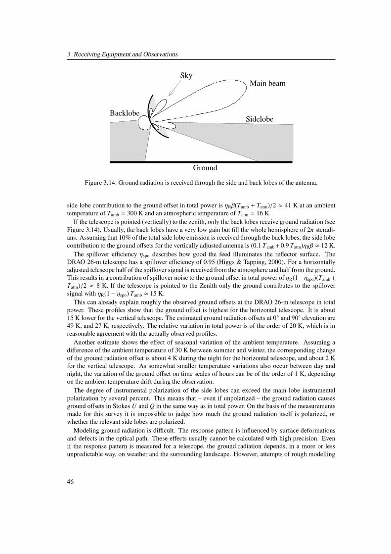
3 Receiving Equipment and Observations
Ground
BacklobeSidelobe
Main beamSky
Figure 3.14: Ground radiation is received through the side and back lobes of the antenna.
side lobe contribution to the ground offset in total power is ηRβ(Tamb + Tatm)/2 ≈ 41 K at an ambienttemperature of Tamb = 300 K and an atmospheric temperature of Tatm = 16 K.
If the telescope is pointed (vertically) to the zenith, only the back lobes receive ground radiation (seeFigure 3.14). Usually, the back lobes have a very low gain but fill the whole hemisphere of 2π steradi-ans. Assuming that 10% of the total side lobe emission is received through the back lobes, the side lobecontribution to the ground offsets for the vertically adjusted antenna is (0.1 Tamb+0.9 Tatm)ηRβ ≈ 12 K.
The spillover efficiency ηspo describes how good the feed illuminates the reflector surface. TheDRAO 26-m telescope has a spillover efficiency of 0.95 (Higgs & Tapping, 2000). For a horizontallyadjusted telescope half of the spillover signal is received from the atmosphere and half from the ground.This results in a contribution of spillover noise to the ground offset in total power of ηR(1−ηspo)(Tamb+
Tatm)/2 ≈ 8 K. If the telescope is pointed to the Zenith only the ground contributes to the spilloversignal with ηR(1 − ηspo) Tamb ≈ 15 K.
This can already explain roughly the observed ground offsets at the DRAO 26-m telescope in totalpower. These profiles show that the ground offset is highest for the horizontal telescope. It is about15 K lower for the vertical telescope. The estimated ground radiation offsets at 0◦ and 90◦ elevation are49 K, and 27 K, respectively. The relative variation in total power is of the order of 20 K, which is inreasonable agreement with the actually observed profiles.
Another estimate shows the effect of seasonal variation of the ambient temperature. Assuming adifference of the ambient temperature of 30 K between summer and winter, the corresponding changeof the ground radiation offset is about 4 K during the night for the horizontal telescope, and about 2 Kfor the vertical telescope. As somewhat smaller temperature variations also occur between day andnight, the variation of the ground offset on time scales of hours can be of the order of 1 K, dependingon the ambient temperature drift during the observation.
The degree of instrumental polarization of the side lobes can exceed the main lobe instrumentalpolarization by several percent. This means that – even if unpolarized – the ground radiation causesground offsets in Stokes U and Q in the same way as in total power. On the basis of the measurementsmade for this survey it is impossible to judge how much the ground radiation itself is polarized, orwhether the relevant side lobes are polarized.
Modeling ground radiation is difficult. The response pattern is influenced by surface deformationsand defects in the optical path. These effects usually cannot be calculated with high precision. Evenif the response pattern is measured for a telescope, the ground radiation depends, in a more or lessunpredictable way, on weather and the surrounding landscape. However, attempts of rough modelling
46
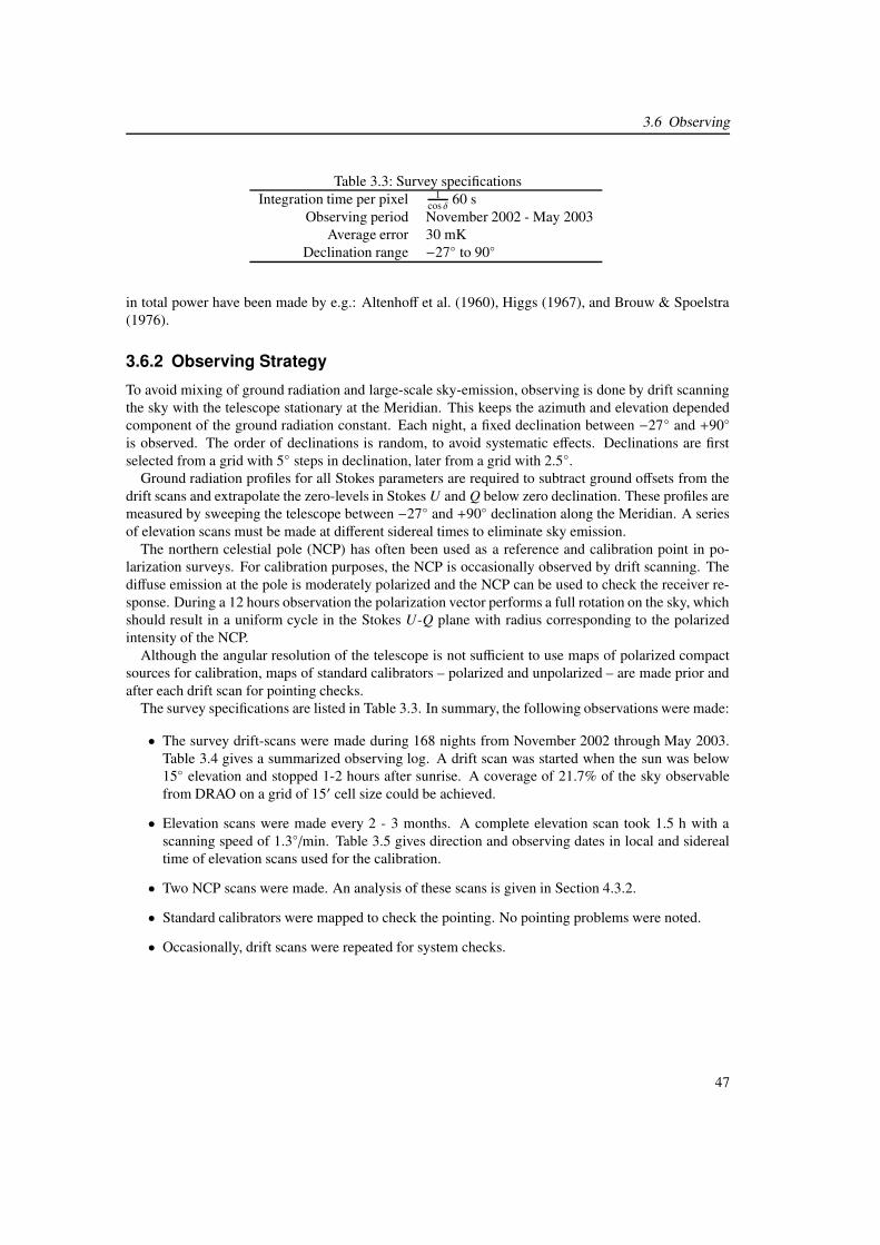
3.6 Observing
Table 3.3: Survey specificationsIntegration time per pixel 1
cos δ 60 sObserving period November 2002 - May 2003
Average error 30 mKDeclination range −27◦ to 90◦
in total power have been made by e.g.: Altenhoff et al. (1960), Higgs (1967), and Brouw & Spoelstra(1976).
3.6.2 Observing Strategy
To avoid mixing of ground radiation and large-scale sky-emission, observing is done by drift scanningthe sky with the telescope stationary at the Meridian. This keeps the azimuth and elevation dependedcomponent of the ground radiation constant. Each night, a fixed declination between −27◦ and +90◦
is observed. The order of declinations is random, to avoid systematic effects. Declinations are firstselected from a grid with 5◦ steps in declination, later from a grid with 2.5◦.
Ground radiation profiles for all Stokes parameters are required to subtract ground offsets from thedrift scans and extrapolate the zero-levels in Stokes U and Q below zero declination. These profiles aremeasured by sweeping the telescope between −27◦ and +90◦ declination along the Meridian. A seriesof elevation scans must be made at different sidereal times to eliminate sky emission.
The northern celestial pole (NCP) has often been used as a reference and calibration point in po-larization surveys. For calibration purposes, the NCP is occasionally observed by drift scanning. Thediffuse emission at the pole is moderately polarized and the NCP can be used to check the receiver re-sponse. During a 12 hours observation the polarization vector performs a full rotation on the sky, whichshould result in a uniform cycle in the Stokes U-Q plane with radius corresponding to the polarizedintensity of the NCP.
Although the angular resolution of the telescope is not sufficient to use maps of polarized compactsources for calibration, maps of standard calibrators – polarized and unpolarized – are made prior andafter each drift scan for pointing checks.
The survey specifications are listed in Table 3.3. In summary, the following observations were made:
• The survey drift-scans were made during 168 nights from November 2002 through May 2003.Table 3.4 gives a summarized observing log. A drift scan was started when the sun was below15◦ elevation and stopped 1-2 hours after sunrise. A coverage of 21.7% of the sky observablefrom DRAO on a grid of 15′ cell size could be achieved.
• Elevation scans were made every 2 - 3 months. A complete elevation scan took 1.5 h with ascanning speed of 1.3◦/min. Table 3.5 gives direction and observing dates in local and siderealtime of elevation scans used for the calibration.
• Two NCP scans were made. An analysis of these scans is given in Section 4.3.2.
• Standard calibrators were mapped to check the pointing. No pointing problems were noted.
• Occasionally, drift scans were repeated for system checks.
47

3 Receiving Equipment and Observations
Table 3.4: Summarized listing of survey drift scans.Month Declination (◦) CommentOct. 2002 60, 65 10 MHz bandpass filtersNov. 2002 70, 75, 80, -25, -20, -15, -10 10 MHz bandpass filters
-5, 0, 5, 10, 15, 20, 25, 30, 35 and software problems40, -25, 45, 50, 55, -22.5, -17.5
Dec. 2002 -12.5, -10, 3.5, 8.5, 13.5, 18.5 Power failures22.5, 27.5, 32.5, 37.5, 42.5, 47.552.5
Jan. 2003 57.5, 62.5, 67.5, 72.5, 77.5, -7.5 Periods of snow-2.5, 2.5, 7, 12, 17, -20, -12.5-7.5, -5, 50, 75, 41, -24, 46, -12.5-15, 51, -19, 56, -14, 10, 40, 2060, 30
Feb. 2003 79, 1, 59, 21, -11, 71, -4, -6, -9 Software and hardware69, 76, 26, 24, 29, 31, 34, 36, 39 modifications-1, -16
Mar. 2003 64, 66, 70, 6, -21, 16, -25, -11, 6 Some snow44, 49, 54, 60, 11, 19, 2, 37, 28,74-2, 23, 13.5, 33, -8, -7, 61.5, 53, -18
Apr. 2003 77, 43, 48, -13, 4, 47, 72, 13, 148, 9, 58, 68, 65, 15, 5, 0, 35, -2257, 38, 61, -3, 85, 25, 45, 52, 18
May 2003 -17, 22, 41.5, 63, -9.5, -12, -4.5-20.5, 27, -19.5, 32, 17.5, 6.5, -14.5-23, 54.5, 11.5, -6, 59.75, -26, -27-28, -29
Table 3.5: Observing dates of the elevation scans used for the determination of ground radiation pro-files.
Date LT LST DirectionDec 12, 2002 18:18 23:36 down
19:26 0:52 up21:00 2:27 down22:37 4:05 up
48
4 Data Processing and AbsoluteCalibration
The data reduction results in Stokes U and Q maps of the northern sky, showing the distributionand strength of polarized emission at 1.4 GHz. To transform the observed correlation productsinto Stokes parameters a calibration is required. The data are then averaged and gridded forscientific analysis. This chapter describes the data reduction steps. A detailed error analysis ispresented at the end of this chapter.
4.1 Reduction Chain
After having discussed the different system adjustments, error sources, and observing methods in theprevious chapter, this chapter gives a detailed description of the data processing and calibration steps– the data reduction. The first processing steps are done with the Data Reduction Program described inSection 3.2.3, for most of the other reduction steps individual glish-scripts are written. A flow diagramillustrating the different stages of data reduction is shown in Figure 4.1.
Three additional surveys for the absolute calibration of the raw data are utilized. The 1.42 GHzStockert 25-m Survey (Reich & Reich, 1986; Reich, 1982) is used for the calibration of the total powerdata, the LDS serves as reference for the calibration of the instrumental response and provides zero-levels in Stokes U and Q, and data from the EMLS made with the Effelsberg 100-m telescope are usedto adjust the Stokes U and Q intensity scales. The resolution and sensitivity of the first two surveysis comparable with the 26-m Survey, whereas the EMLS has a higher angular resolution and bettersensitivity.
4.1.1 Radio Frequency Interference Flagging
The first reduction step is the flagging of data corrupted by RFI. Flagging in this context means thatdata affected by RFI are “marked” by a search routine and excluded from further data processing. Theenormous amount of data does not allow a visual – by hand – flagging, instead, an automated flaggingroutine is developed.
RFI is mainly generated by terrestrial radio transmitters, radar, or locally operating devices, whichmay produce a spectrum of harmonic lines. Satellites, although supposed to transmit outside the pro-tected band from 1, 400 to 1, 427 MHz, may also generate RFI in the protected band. Even if trans-mitting at frequencies outside the observing band, strong radio transmitters can push the LNAs intosaturation and thus affect the system gain. Figure 4.2 shows an extreme RFI event several seconds ofduration. Most of the observed RFI is shorter in time and usually only a few integrations (between ∼ 1and ∼ 10) are affected.
The remote observatory site is surrounded by mountains which block the terrestrial RFI to someextent. In addition, the institute buildings are screened by a Faraday cage, which reduces most of theRFI caused by local computers and backend devices. Therefore, the DRAO provides ideal conditionsfor radio observations in the L-band. In fact, only 0.1% of the total observing time is lost due to
49
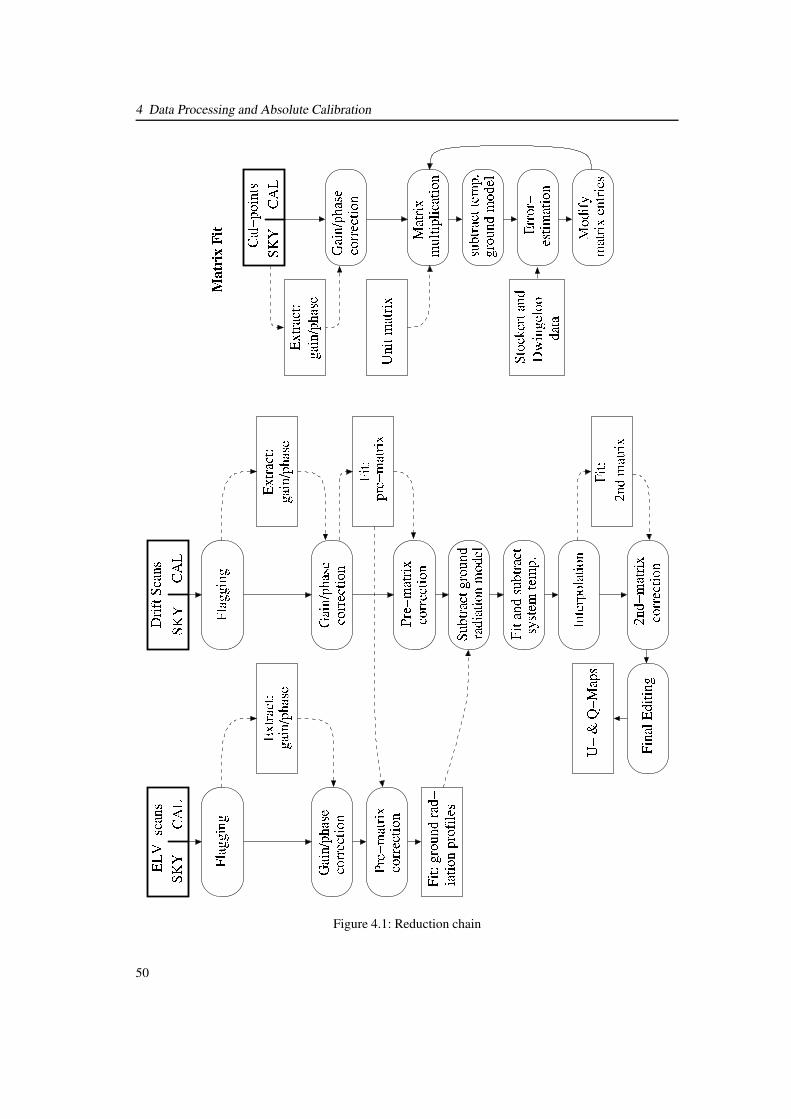
4 Data Processing and Absolute Calibration
Figure 4.1: Reduction chain
50
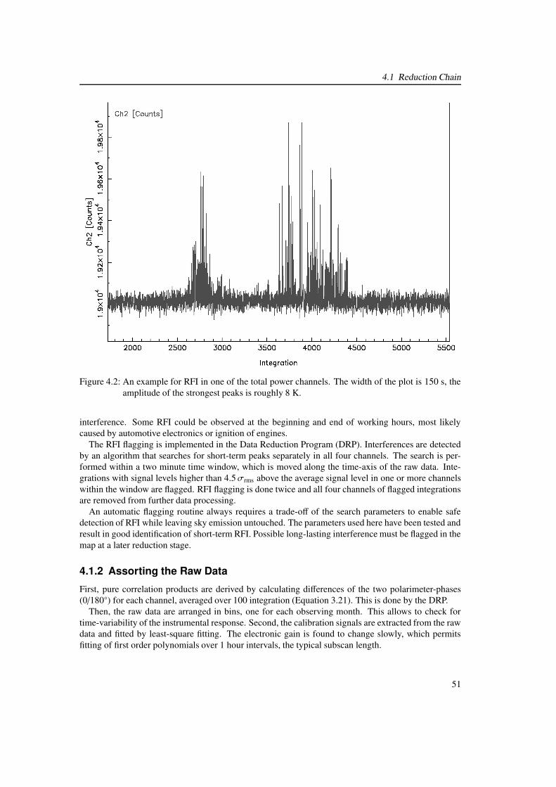
4.1 Reduction Chain
Figure 4.2: An example for RFI in one of the total power channels. The width of the plot is 150 s, theamplitude of the strongest peaks is roughly 8 K.
interference. Some RFI could be observed at the beginning and end of working hours, most likelycaused by automotive electronics or ignition of engines.
The RFI flagging is implemented in the Data Reduction Program (DRP). Interferences are detectedby an algorithm that searches for short-term peaks separately in all four channels. The search is per-formed within a two minute time window, which is moved along the time-axis of the raw data. Inte-grations with signal levels higher than 4.5σrms above the average signal level in one or more channelswithin the window are flagged. RFI flagging is done twice and all four channels of flagged integrationsare removed from further data processing.
An automatic flagging routine always requires a trade-off of the search parameters to enable safedetection of RFI while leaving sky emission untouched. The parameters used here have been tested andresult in good identification of short-term RFI. Possible long-lasting interference must be flagged in themap at a later reduction stage.
4.1.2 Assorting the Raw Data
First, pure correlation products are derived by calculating differences of the two polarimeter-phases(0/180◦) for each channel, averaged over 100 integration (Equation 3.21). This is done by the DRP.
Then, the raw data are arranged in bins, one for each observing month. This allows to check fortime-variability of the instrumental response. Second, the calibration signals are extracted from the rawdata and fitted by least-square fitting. The electronic gain is found to change slowly, which permitsfitting of first order polynomials over 1 hour intervals, the typical subscan length.
51
4 Data Processing and Absolute Calibration
Implemented in the sorting script is a checking routine for the telescope position. Observationswere usually done unattended and accidental telescope movements due to snow or wind may not berecognized. Therefore, the hour angle and declination of each scan is checked and observations areflagged out if necessary.
Additional observations such as elevation scans, NCP measurements, and maps require a somewhatdifferent procedure. Elevation scans, for example, require higher order polynomial fits of the extractedcalibration signals, because the receiver shows an elevation-dependend gain. Moreover, the coordinatesof manually performed observations, such as NCP scans, must be derived from the LST recordings,because the coordinates provided by the telescope control system are wrong in that case.
4.1.3 Electronic Gain
The cal signal is periodically injected into the signal path and is used to track electronic gain fluctua-tions. The intrinsic polarized intensity PIstandard and polarization angle PAstandard of the cal is assumedconstant over the observing term. Hence, variations of the measured polarized intensity PIcal and po-larization angle PAcal of the cal must be interpreted as gain and phase drifts within the receiver.
With the separated sky and fitted cal signals the data can be corrected for electronic gain fluctuations.The total power channels are multiplied with the reciprocal of the measured cal signal strengths and thepolarization channels are rotated and normalized according to PIcal and PAcal:
RR′sky = RRsky/RRcal
LL′sky = LLsky/LLcal
RL′sky =(
RLsky cos 2PAcal − LRsky sin 2PAcal
)
/PIcal
LR′sky =(
LRsky cos 2PAcal + RLsky sin 2PAcal
)
/PIcal.
(4.1)
RRcal and LLcal are the measured strength of the cal in total power and RLcal and LRcal the ampli-tudes in the sine- and cosine-channel. Polarized intensity and angle of the cal are given by PIcal =(
RL2cal + LR2
cal
)0.5and PAcal = 0.5 arctan
(
RLcalLRcal
)
.Although the precise strength and polarization angle of the noise source is unknown and not relevant
at this point, a rough estimate of PIstandard and PAstandard can be derived by applying the matrices 4.5and 4.6 to the measured values. By this, the cal signal is found to have the following approximatestrength:
< PIstandard >= 41 K< PAstandard >= 71◦, (4.2)
with the polarization angle given in the RA-DEC coordinate system.Because of the intensity of the noise source, all integrations with the cal signal switched on are used
only for the determination of the electronic gain and are excluded from further data processing. Thismeans that the noise source injection reduces the effective observing time. Therefore a trade-off atthe beginning of the observing run was made: 1.7% of the total observing time is used for systemcalibration.
4.1.4 Pre-Calibration
The polarimeter provides outputs that are proportional to the two auto- and cross-correlations of the Rand L-signals: RR, LL, RL, and LR. The intention of the pre-calibration is to convert the arbitrary scale-unit of the polarimeter outputs (counts) into a temperature scale. The total power channels (RR, LL)are calibrated to approximate brightness temperature and the cross-correlations (RL, LR) are scaled
52
4.1 Reduction Chain
and rotated to roughly express Stokes U and Q measured in Kelvin. This step does not include anycorrection of instrumental errors such as instrumental cross-talk.
The polarimeter output channels form a 4-vector. Scaling and rotation of this vector is computedby multiplication with a 4 × 4-matrix, the pre-calibration matrix. The entries on the main diagonal ofthis matrix are mere scaling factors, whereas the 2 × 2-submatrix causes a rotation of RL and LR. Theother entries are zero. The computation of the pre-calibration matrix is done in an intermediate step byiterative fitting.
Iterative Determination of the Pre-Calibration Matrix
The Stockert Survey (Stokes I) is calibrated in full-beam brightness temperature, which must be con-verted into main-beam brightness temperature, whereas the LDS gives Stokes U and Q brightnesstemperatures. The reference values for the computation of the pre-calibration matrix are given by:
RRref =(
0.5 · 1.55 (IStockert − 2.8 K))
+ 2.8 KLLref =
(
0.5 · 1.55 (IStockert − 2.8 K))
+ 2.8 KRLref = ULDS
LRref = QLDS,
(4.3)
which includes the transformation of full-beam into main-beam brightness temperature of the StockertSurvey. Stokes V is assumed zero.
The fitting problem can be expressed as follows: Each pointing n that has been observed with allthree telescopes – DRAO 26-m, Stockert and Dwingeloo – results in an equation according to:
M1′ ·
RRLLRLLR
raw,n
=
RRLLRLLR
ref,n
, (4.4)
with “raw” referring to the uncalibrated DRAO 26-m data. Hence, if the total number of pointings ism, this results in a set of m equations with n = 1, 2, . . . ,m− 1,m. By fitting the matrix entries m′11, m′22,m′33, m′44, m′34 and m′43 of the matrixM′1 by minimization of the difference between corrected raw dataand reference values, the best solution of the set of m equations is found.
Determination of the matrix entries must be done by iterative fitting and cannot be achieved byleast-square fitting. This is because the raw data are not corrected for ground radiation and systemtemperature drifts at this point. A least-square fit1 is therefore not possible because RRraw, LLraw,RLraw, LRraw still contain time and declination dependend offsets. These offsets must be approximatedduring fitting as done in the following algorithm (see Fig. 4.1 on the right):
1. The DRAO 26-m raw data of congruent pointings are corrected for electronic gain.
2. The initial matrixM′1 is set to be the unit matrix.
3. The DRAO 26-m raw data are corrected my multiplication withM′1 according to Equation 4.8.
1e.g. in this case applied to the following set of equations in order to obtain the coefficients m′:
RRref,{1...n} = m′11 RRraw,{1...n}LLref,{1...n} = m′22 LLraw,{1...n}RLref,{1...n} = m′33 RLraw,{1...n} + m′34 LRraw,{1...n}LRref,{1...n} = m′43 RLraw,{1...n} + m′44 LRraw,{1...n}
53
4 Data Processing and Absolute Calibration
4. Ground radiation and system temperature drifts are approximately removed by subtracting alinear baseline fitted through all congruent pointings lying on the same declination.
5. The fit-error is given as the sum of the squared differences between corrected DRAO 26-m dataand the reference values.
6. Matrix entries ofM′1 are either randomly altered and the iteration continues at point three or theiteration is stopped if the minimization of the fit-error is achieved.
Pre-calibration matrices are computed individually for each observing month. About m = 100 to 140pointings with congruity of the pointing centres of ≤ 21′ in all three surveys could be extracted for eachobserving month. The number of matches is mainly limited by the sparse number of data points fromthe LDS. Throughout the observing term a total of 860 matches was obtained. No time-dependence ofthe pre-calibration matrix was found.
Pre-Calibration of Raw Data
To account for an IF-filter change in November 2003, two different pre-calibration matrices were de-termined. The following matrices are used for the pre-calibration of the data:
Nov 2003 : M′1 =
11.0 0 0 00 12.0 0 00 0 −16.35 50.190 0 54.16 18.04
(4.5)
and
Dec 2003 −May 2004 : M′1 =
9.08 0 0 00 8.55 0 00 0 −16.35 50.190 0 54.16 18.04
, (4.6)
with errors of the matrix entries as follows:
Errors : ∆M′1,2 =
0.4 0 0 00 0.3 0 00 0 3.9 3.50 0 3.0 3.1
. (4.7)
The matrices show only small differences in the scaling factors of the total power channels for the twopairs of IF filters.
These matrices are applied to the raw data by computing the following matrix multiplication for eachintegration:
RRLLRLLL
corr
=M′1 ·
RRLLRLLL
raw
. (4.8)
The pre-calibration is the first iteration step of an iterative determination of the instrumental Müllermatrix. The second iteration step follows in Section 4.1.10.
54

4.1 Reduction Chain
4.1.5 Ground Radiation
Elevation scans were made periodically during the observing term. Like the survey raw-data, elevationscans are corrected for electronic gain and converted into brightness temperature. Ground radiationprofiles for each channel are determined on the basis of elevation scans. Using the derived profiles thesurvey data are then corrected for ground radiation.
Determination of Ground Radiation Profiles
Four elevation scans are of high enough quality to be used for the determination of ground radiationprofiles. Other elevation scans are either corrupted by gain jumps or showed strong sky contribution.The selected scans are first stacked, supposing that the averaged profiles in Stokes U and Q and thelower envelope in the total power channels roughly represent pure ground radiation. This is justifiedas the scans were taken at different sidereal times. The stacked profiles are then averaged along theelevation axis in bins of 7.◦5 and fitted by a “spline”-function which should further minimize remainingsky emission. Although the scans used cover a bright polarized region, the averaged scans representuseful ground profiles.
Figure 4.3 shows the derived ground radiation profiles. The offset of the total power profiles is about161 K at the minimum, which gives the system temperature without sky emission. The mean offsets ofabout 3.5 K in the Stokes-U-profile and −3.7 K in the Q-profile may indicate:
1. remaining phase and gain mismatches in the pre-hybrid part,
2. correlated receiver noise caused by cross-talk or backcoupling,
3. polarized backlobes of the telescope, picking up ground radiation.
The first can be excluded from the system check; more likely are the second and third. Also interestingis the north-south asymmetry about 90◦ elevation of the U and Q profiles, which may be due to themultipole structure of a telescope’s response pattern to unpolarized radiation. The bump in the totalpower profiles at about 90◦ elevation may be spillover noise, which should be highest for the telescopepointing towards the Zenith.
Subtraction of Ground Radiation
Subtraction of ground radiation is straightforward. The ground offsets for each declination and chan-nel are taken from the profiles. These offsets are then subtracted from the drift scans. This way, thedeclination-dependend component is removed and only the time-variable component of ground radia-tion and system temperature is left, which is corrected later in Section 4.1.8
The LDS provides absolutely calibrated reference points only for declinations above 0◦, at which, inprinciple, the 26-m Survey could be calibrated without ground radiation profiles2. Below 0◦, profilesare essential to set correct zero-levels in Stokes U and Q.
4.1.6 Gridding
Integrations are averaged and binned into a grid of equatorial coordinates with 15′ cell size, which issomewhat less then the telescope’s HPBW/2 required for full Nyquist sampling. No particular weight-ing scheme is used; integrations are uniformly weighted and averaged across the cell. The griddingsignificantly reduces the amount of data.
2which has not been tested though
55

4 Data Processing and Absolute Calibration
30 50 70 90 70 50Elevation
-3,8
-3,6
-3,4
Stokes Q
30 50 70 90 70 50Elevation
2,5
3
3,5
4
4,5
TB (K
)
Stokes U
30 50 70 90 70 50160
165
170
175
180TP 2
30 50 70 90 70 50160
165
170
175
180
TB (K
)TP 1
NS NS
NSNS
Figure 4.3: Ground radiation profiles determined on the basis of elevation scans, shown for total power(upper panels) and polarization (bottom panels). An explanation for the north-south asym-metry is given in the text.
4.1.7 Solar Interference and Ionospheric Faraday Rotation
Aside from automatic RFI flagging, which is done in the first step (Section 4.1.1), the data are nowvisually inspected for solar interference and ionospheric Faraday rotation. A graphical program waswritten to display and manually flag corrupted data. Whenever day-time data were used, drift scanswere cross-checked with neighboring scans to recognize high levels of ionospheric Faraday rotation orsolar interference. Only some of the day-time data show apparent solar interference and needed to beflagged. No indication was found for ionospheric Faraday rotation at night.
4.1.8 System Temperature Fluctuations
The correction of fluctuations of the system temperature turns out to be a crucial step in the data cal-ibration. These fluctuations are possibly caused by variations of the ground radiation offsets duringthe observation. In the final map these fluctuations show up as stripes in total power and polarizationand must be removed for calibration. Existing de-striping programs (e.g. NOD2 reduction package ofthe Effelsberg 100-m telescope) are not suitable and appropriate correction software thus needed to bewritten.
While the receiver-noise temperature is determined by ohmic losses in the receiving system andshould therefore be rather constant, a gradual time-variability of the ground-noise temperature is ex-
56
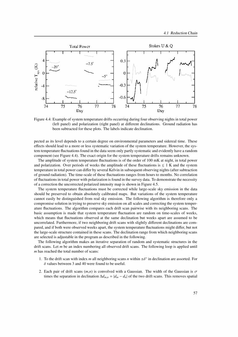
4.1 Reduction Chain
Figure 4.4: Example of system temperature drifts occurring during four observing nights in total power(left panel) and polarization (right panel) at different declinations. Ground radiation hasbeen subtracted for these plots. The labels indicate declination.
pected as its level depends to a certain degree on environmental parameters and sidereal time. Theseeffects should lead to a more or less systematic variation of the system temperature. However, the sys-tem temperature fluctuations found in the data seem only partly systematic and evidently have a randomcomponent (see Figure 4.4). The exact origin for the system temperature drifts remains unknown.
The amplitude of system temperature fluctuations is of the order of 100 mK at night, in total powerand polarization. Over periods of weeks the amplitude of these fluctuations is . 1 K and the systemtemperature in total power can differ by several Kelvin in subsequent observing nights (after subtractionof ground radiation). The time-scale of these fluctuations ranges from hours to months. No correlationof fluctuations in total power with polarization is found in the survey data. To demonstrate the necessityof a correction the uncorrected polarized intensity map is shown in Figure 4.5.
The system temperature fluctuations must be corrected while large-scale sky emission in the datashould be preserved to obtain absolutely calibrated maps. But variations of the system temperaturecannot easily be distinguished from real sky emission. The following algorithm is therefore only acompromise solution in trying to preserve sky emission on all scales and correcting the system temper-ature fluctuations. The algorithm compares each drift scan pairwise with its neighboring scans. Thebasic assumption is made that system temperature fluctuation are random on time-scales of weeks,which means that fluctuations observed at the same declination but weeks apart are assumed to beuncorrelated. Furthermore, if two neighboring drift scans with slightly different declinations are com-pared, and if both were observed weeks apart, the system temperature fluctuations might differ, but notthe large-scale structure contained in these scans. The declination range from which neighboring scansare selected is adjustable in the program as described in the following.
The following algorithm makes an iterative separation of random and systematic structures in thedrift scans. Let m be an index numbering all observed drift scans. The following loop is applied untilm has reached the total number of scans:
1. To the drift scan with index m all neighboring scans n within ±δ◦ in declination are assorted. Forδ values between 3 and 40 were found to be useful.
2. Each pair of drift scans (m,n) is convolved with a Gaussian. The width of the Gaussian is σtimes the separation in declination ∆dm,n = |dm − dn| of the two drift scans. This removes spatial
57
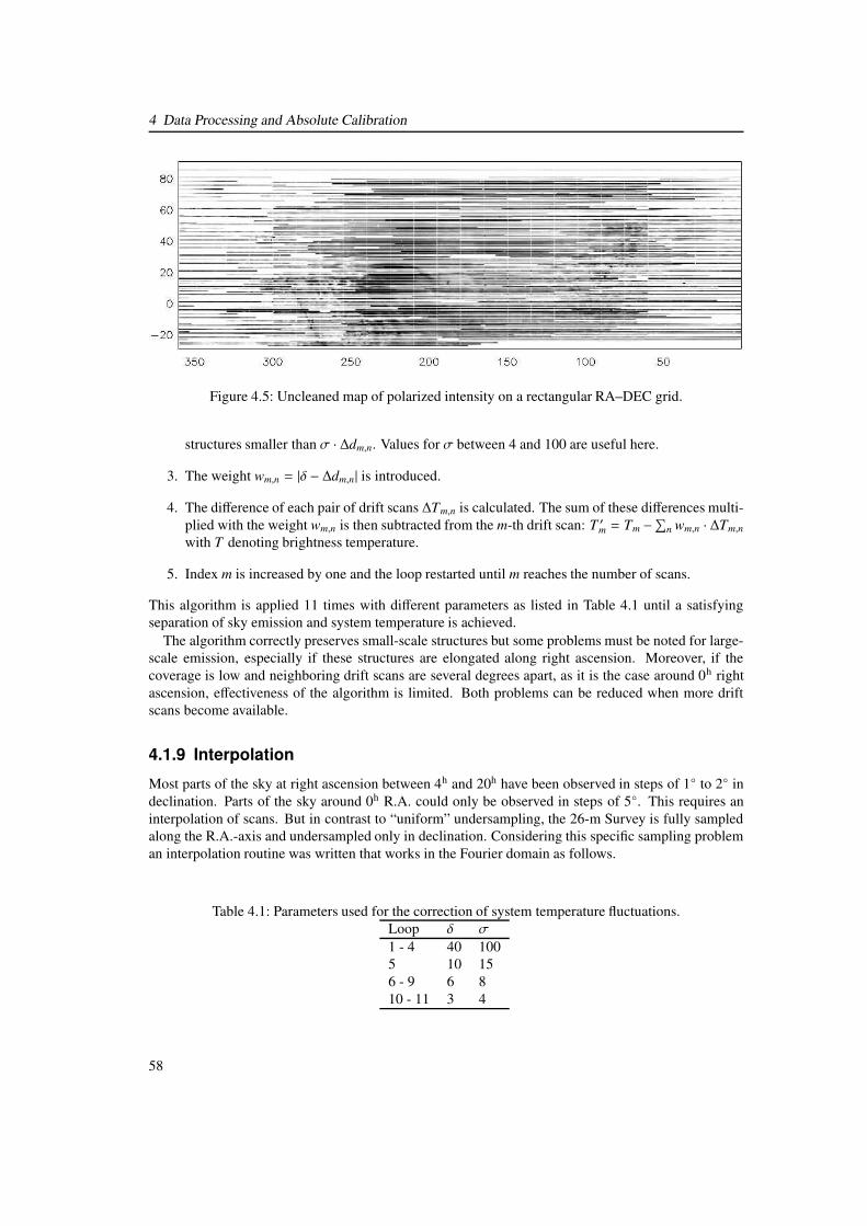
4 Data Processing and Absolute Calibration
Figure 4.5: Uncleaned map of polarized intensity on a rectangular RA–DEC grid.
structures smaller than σ · ∆dm,n. Values for σ between 4 and 100 are useful here.
3. The weight wm,n = |δ − ∆dm,n| is introduced.
4. The difference of each pair of drift scans ∆Tm,n is calculated. The sum of these differences multi-plied with the weight wm,n is then subtracted from the m-th drift scan: T ′m = Tm −
∑
n wm,n · ∆Tm,n
with T denoting brightness temperature.
5. Index m is increased by one and the loop restarted until m reaches the number of scans.
This algorithm is applied 11 times with different parameters as listed in Table 4.1 until a satisfyingseparation of sky emission and system temperature is achieved.
The algorithm correctly preserves small-scale structures but some problems must be noted for large-scale emission, especially if these structures are elongated along right ascension. Moreover, if thecoverage is low and neighboring drift scans are several degrees apart, as it is the case around 0h rightascension, effectiveness of the algorithm is limited. Both problems can be reduced when more driftscans become available.
4.1.9 Interpolation
Most parts of the sky at right ascension between 4h and 20h have been observed in steps of 1◦ to 2◦ indeclination. Parts of the sky around 0h R.A. could only be observed in steps of 5◦. This requires aninterpolation of scans. But in contrast to “uniform” undersampling, the 26-m Survey is fully sampledalong the R.A.-axis and undersampled only in declination. Considering this specific sampling probleman interpolation routine was written that works in the Fourier domain as follows.
Table 4.1: Parameters used for the correction of system temperature fluctuations.Loop δ σ
1 - 4 40 1005 10 156 - 9 6 810 - 11 3 4
58

4.1 Reduction Chain
The drifts scans are Fourier transformed, using the DFT3-algorithm of AIPS++. Unobserved decli-nations are filled by linear interpolation of the Fourier transformed drift scans. The interpolated scansare then reverse transformed into the image plane. This algorithm does not affect observed scans sothat it is possible to extract the original observations from the interpolated map.
In a second interpolation step, a few remaining pixels at the map edges, which could not be interpo-lated in the Fourier domain, are interpolated in the image plane. These pixels are replaced by the meanof neighboring pixels, weighted with the inverse of the distance.
For test purposes the data have also been interpolated employing a number of available programs(e.g. NOD2 routines, GILDAS software), which interpolate in the image plane. These algorithms oftencalculate means of pixel values using more or less sophisticated weighting schemes. It was found thatthe Fourier interpolation preserves the large-scale structure better than an interpolation in the imageplane. However, each kind of analysis should imply a proper way of doing the interpolation, if requiredfor the scientific purpose at all. Therefore it is planned to make the 26-m Survey publicly available inform of Fourier interpolated maps as well as individual drift scans.
4.1.10 Second Calibration
Up to this reduction step the data are not corrected for instrumental cross-talk. This, and a moreaccurate scaling and rotation of the RL and LR scales, is computed in the following. Similar as forthe pre-calibration, a correction matrix is applied to the 4-vector formed from the four polarimeterchannels. No further corrections of the total power data are made as the intention is the measurementof polarization. Instead of iterative fitting, least-square fitting can now be applied because the raw dataare already corrected for electronic gain and ground radiation. The reference points are again takenfrom the Leiden-Dwingeloo polarization survey.
A single calibration matrix is determined for the whole data set. The following correction matrixM′2
is found:
M′2 =
1 0 0 00 1 0 0
0.025 −0.023 1.12 0.050.014 −0.041 0.05 1.03
, (4.9)
with errors of ±0.01 of the matrix entries. Raw data are corrected according to Equation 4.8. Thescaling correction caused by the second calibration is small – scaling factors are around unity. Cross-talk values of 0.2% in Stokes U (RL) and −2.7% in Q (LR) are found.
4.1.11 Final Editing
A manual editing of the final Stokes U and Q maps is unavoidable. This editing involves the followingsteps:
1. The program that corrects system temperature fluctuations (Section 4.1.8) works in a rectangulargrid of equatorial coordinates. This program assumes that drift scans run from 0h to 24h in rightascension. After subtraction of system temperature, discontinuities at 0 hour are left. Thesejumps are of the order . 30 mK and corrected by baseline adjustment within a 2h right ascensioninterval between 23h and 1h.
2. Although the automated flagging routine (Section 4.1.1) flagged most of the RFI correctly, a fewspikes in the data must be edited by hand. By utilizing available software packages, the Stokes U
3Discrete Fourier Transformation
59
4 Data Processing and Absolute Calibration
and Q maps are displayed (using kview4) and a bad pixel mask created. Bad pixels are replacedby interpolated pixel values (iraf 5, task: fixpix).
3. The final Stokes U and Q maps are smoothed with a Gaussian beam to remove sub-beam struc-tures. The FWHM of the Gaussian is 36′. If the smoothing is done within a rectangular gridof equatorial coordinates, the FWHM beam must be adapted to the declination (FWHM =
36′/ cos δ).
4.2 Refinement of Temperature Scale
A comparison of the 26-m Survey with polarization data taken from the EMLS reveals a mismatchof both brightness temperature scales. Temperatures from the 26-m Survey are systematically toohigh by a factor of 1.18 ± 0.03 compared with the EMLS. An overestimation of the Dwingeloo main-beam temperature scale must be assumed, because the calibration scheme ties the 26-m Survey to theDwingeloo survey. A possible reason for the inaccuracy is that the LDS itself was calibrated merelyagainst two calibration points, of which polarized intensities were known only to some precision.
The data used for the comparison of brightness temperatures are taken from two regions: a 35◦ × 35◦
large map towards Cassiopeia-A and a 40◦×16◦ large map toward the Taurus-Auriga-Perseus molecularclouds. These are preliminary maps from the EMLS, which are covered by 28 drift scans from the 26-mSurvey.
As the EMLS lacks large-scale emission (see Chapter 1) a direct comparison with the 26-m Survey istherefore not meaningful. As a solution, missing large-scale structures in the EMLS are approximatedby polynomials of first to third order. The coefficients of these polynomials and the scaling factor of the26-m temperature scale are then fitted to the Effelsberg data, with the difference between EMLS and26-m Survey to be minimized. Figure 4.6 shows two example scans used for this comparison.
It is certain that the main-beam temperature scale of the EMLS is determined more accurately thanthat of the LDS. Because of the higher sensitivity of the Effelsberg 100-m telescope, standard calibrationsources with well known fluxes can be used for calibration. This is almost impossible with small-diameter telescopes and uncooled receivers. Therefore, the temperature scale of the 26-m Survey isre-calibrated against the EMLS temperature scale which, in turn, is determined on the basis of standardcalibrators. Hence, temperatures quoted in the 26-m Survey conform to the Effelsberg main-beambrightness temperatures scale.
4.3 Error Analysis
Several error sources contribute to the error budget of the 26-m Survey. The relevance of the followingerrors and their influence on the final Stokes U and Q maps must be discussed:
1. Errors of the entries in the system Müller matrix cause systematic errors in the data. Consideringpre-calibration and second matrix the error is estimated to be ∼ 6%.
2. Non-circular response of the receiver to polarized signals.
3. Uncorrected instrumental polarization caused by sources received through the side lobes.
4. Errors in the LDS.4kview is part of the karma toolkit (http://www.atnf.csiro.au/computing/software/karma/)5iraf: Image Reduction and Analysis Facility (http://iraf.noao.edu/)
60

4.3 Error Analysis
55 60 65 70 75 80-200
-100
0
100
200
300
Stok
es U
(mK
)
Taurus Field
360 365 370 375-200
-100
0
100
200Cas-A Field
55 60 65 70 75 80Right Acension
-300
-200
-100
0
100
200
Stok
es Q
(mK
)
360 365 370 375Right Ascension
0
100
200
Figure 4.6: Two example scans through the Taurus complex (left panels) and Cassiopeia-A (right pan-els). The dashed lines show EMLS data and the solid lines 26-m Survey data. The missinglarge-scale emission in the EMLS data is approximated by polynomials. The DRAO 26-mdata are divided by 1.18.
5. Sudden changes of environmental parameters such as humidity, ambient temperature, etc. affectthe system temperature and telescope gain. Affected data must be flagged. If the effects inStokes U and Q are smaller then 10 mK, they are unlikely to be detected in view of the noiselevel and increase the error.
6. System temperature fluctuations are corrected by a program (Section 4.1.8). To a certain de-gree this program confuses structures elongated along right ascension with system temperaturefluctuations. This may cause errors of about . 30 mK as derived from simulations.
7. Below 0◦, errors in the ground radiation profiles causes incorrect zero-levels in U and Q. Becauseof the averaging and fitting of several elevation scans, these errors are certainly below 50 mK.
4.3.1 The System Müller Matrix
To investigate the system properties a Müller matrix for the telescope is calculated. Only the secondcalibration matrix (Equation 4.9) is considered, because the pre-calibration matrix does a scaling androtation. Moreover, as for the calibration the basis consisting of RR, LL, RL, and LR is used, the secondcalibration matrix must be transformed into a Müller matrix to be applicable to Stokes parameters.
61
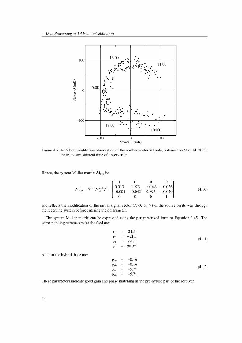
4 Data Processing and Absolute Calibration
-100 0 100Stokes U (mK)
-100
0
100
Stok
es Q
(mK
)
11:00
15:00
17:0019:00
13:00
Figure 4.7: An 8 hour night-time observation of the northern celestial pole, obtained on May 14, 2003.Indicated are sidereal time of observation.
Hence, the system Müller matrixMsys is:
Msys = T−1M′−1
2 T =
1 0 0 00.013 0.973 −0.043 −0.026−0.001 −0.043 0.895 −0.020
0 0 0 1
(4.10)
and reflects the modification of the initial signal vector (I, Q, U, V) of the source on its way throughthe receiving system before entering the polarimeter.
The system Müller matrix can be expressed using the parameterized form of Equation 3.45. Thecorresponding parameters for the feed are:
ε1 = 21.3ε2 = −21.3φ1 = 89.8◦
φ2 = 90.3◦.
(4.11)
And for the hybrid these are:gya = −0.16gxb = −0.16φya = −5.7◦
φxb = −5.7◦.
(4.12)
These parameters indicate good gain and phase matching in the pre-hybrid part of the receiver.
62
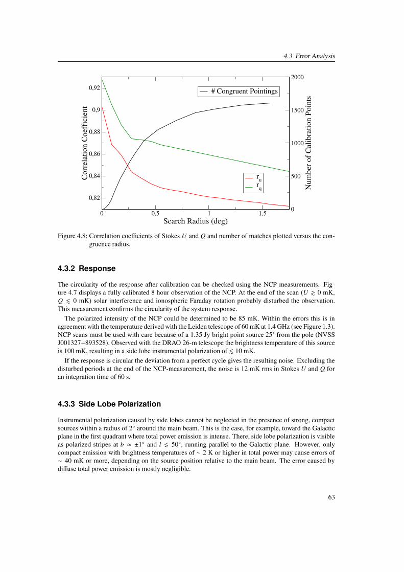
4.3 Error Analysis
0 0,5 1 1,5Search Radius (deg)
0,82
0,84
0,86
0,88
0,9
0,92C
orre
latio
n C
oeff
icie
nt
rurq
0
500
1000
1500
2000
Num
ber o
f Cal
ibra
tion
Poin
ts
# Congruent Pointings
Figure 4.8: Correlation coefficients of Stokes U and Q and number of matches plotted versus the con-gruence radius.
4.3.2 Response
The circularity of the response after calibration can be checked using the NCP measurements. Fig-ure 4.7 displays a fully calibrated 8 hour observation of the NCP. At the end of the scan (U & 0 mK,Q . 0 mK) solar interference and ionospheric Faraday rotation probably disturbed the observation.This measurement confirms the circularity of the system response.
The polarized intensity of the NCP could be determined to be 85 mK. Within the errors this is inagreement with the temperature derived with the Leiden telescope of 60 mK at 1.4 GHz (see Figure 1.3).NCP scans must be used with care because of a 1.35 Jy bright point source 25′ from the pole (NVSSJ001327+893528). Observed with the DRAO 26-m telescope the brightness temperature of this sourceis 100 mK, resulting in a side lobe instrumental polarization of . 10 mK.
If the response is circular the deviation from a perfect cycle gives the resulting noise. Excluding thedisturbed periods at the end of the NCP-measurement, the noise is 12 mK rms in Stokes U and Q foran integration time of 60 s.
4.3.3 Side Lobe Polarization
Instrumental polarization caused by side lobes cannot be neglected in the presence of strong, compactsources within a radius of 2◦ around the main beam. This is the case, for example, toward the Galacticplane in the first quadrant where total power emission is intense. There, side lobe polarization is visibleas polarized stripes at b ≈ ±1◦ and l . 50◦, running parallel to the Galactic plane. However, onlycompact emission with brightness temperatures of ∼ 2 K or higher in total power may cause errors of∼ 40 mK or more, depending on the source position relative to the main beam. The error caused bydiffuse total power emission is mostly negligible.
63
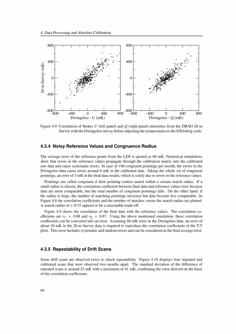
4 Data Processing and Absolute Calibration
-800 -400 0 400 800Dwingeloo - U (mK)
-800
-400
0
400
80026
-m S
urve
y (m
K)
-800 -400 0 400 800Dwingeloo - Q (mK)
-800
-400
0
400
800
Figure 4.9: Correlation of Stokes U (left panel) and Q (right panel) intensities from the DRAO 26-mSurvey with the Dwingeloo survey before adjusting the temperatures to the Effelsberg scale.
4.3.4 Noisy Reference Values and Congruence Radius
The average error of the reference points from the LDS is quoted as 60 mK. Numerical simulationsshow that errors in the reference values propagate through the calibration matrix into the calibratedraw data and cause systematic errors. In case of 100 congruent pointings per month, the errors in theDwingeloo data cause errors around 6 mK in the calibrated data. Taking the whole set of congruentpointings, an error of 3 mK in the final data results, which is solely due to errors in the reference values.
Pointings are called congruent if their pointing centres match within a certain search radius. If asmall radius is chosen, the correlation coefficient between final data and reference values rises becausedata are more comparable, but the total number of congruent pointings falls. On the other hand, ifthe radius is large, the number of matching pointings increases but data become less comparable. InFigure 4.8 the correlation coefficients and the number of matches versus the search radius are plotted.A search radius of ≤ 0.◦35 appears to be a reasonable trade-off.
Figure 4.9 shows the correlation of the final data with the reference values. The correlation co-efficients are rU = 0.88 and rQ = 0.87. Using the above mentioned simulation, these correlationcoefficients can be converted into an error. Assuming 60 mK error in the Dwingeloo data, an error ofabout 30 mK in the 26-m Survey data is required to reproduce the correlation coefficients of the T-Tplots. This error includes systematic and random errors and can be considered as the final average error.
4.3.5 Repeatability of Drift Scans
Some drift scans are observed twice to check repeatability. Figure 4.10 displays four repeated andcalibrated scans that were observed two months apart. The standard deviation of the difference ofrepeated scans is around 25 mK with a maximum of 41 mK, confirming the error derived on the basisof the correlation coefficients.
64
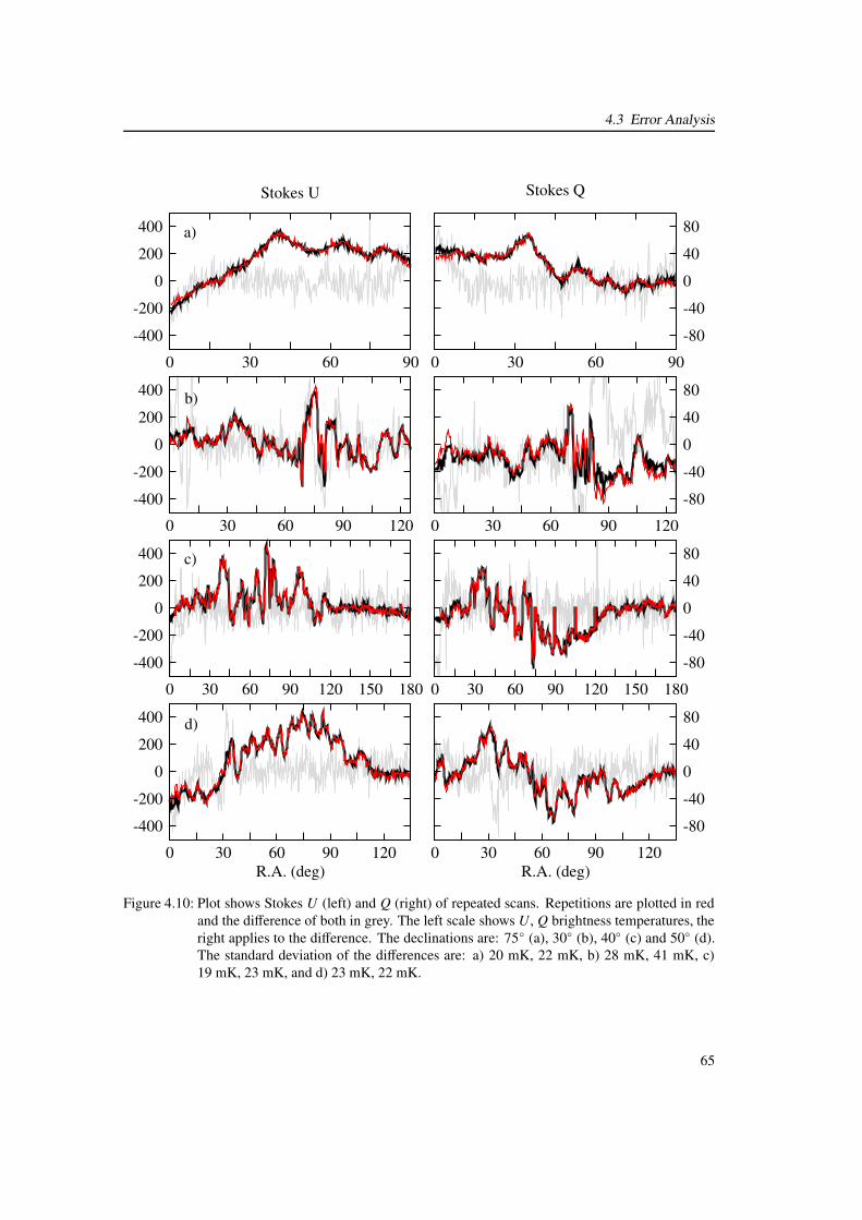
4.3 Error Analysis
0 30 60 90
-400
-200
0
200
400
Stokes U
0 30 60 90
0
-40
-80
40
80
Stokes Q
0 30 60 90 120
-400
-200
0
200
400
0 30 60 90 120
0
-40
-80
40
80
0 30 60 90 120 150 180
-400
-200
0
200
400
0 30 60 90 120 150 180
0
-40
-80
40
80
0 30 60 90 120R.A. (deg)
-400
-200
0
200
400
0 30 60 90 120R.A. (deg)
0
-40
-80
40
80
c)
b)
a)
d)
Figure 4.10: Plot shows Stokes U (left) and Q (right) of repeated scans. Repetitions are plotted in redand the difference of both in grey. The left scale shows U, Q brightness temperatures, theright applies to the difference. The declinations are: 75◦ (a), 30◦ (b), 40◦ (c) and 50◦ (d).The standard deviation of the differences are: a) 20 mK, 22 mK, b) 28 mK, 41 mK, c)19 mK, 23 mK, and d) 23 mK, 22 mK.
65

4 Data Processing and Absolute Calibration
Table 4.2: Error budget of the 26-m Survey.Contribution Error ∆T CommentSystem Matrix ∼ 6%Response 0 mK response is circularSide Lobe Polarization . 40 mK only for compact sourcesReference Values 3 mKWeather . 10 mK if undetectedTsys-Correction . 30 mK up to ∼ 100 mK (see text)Ground Radiation Profiles . 50 mK below 0◦ declinationRms-Noise 12 mK from NCP scan
4.3.6 Final Error
Summing up the above mentioned error contributions, an error budget (Table 4.2) can be stated. A directmeasurement of the rms-noise of 12 mK per 60 s integration was derived from the NCP measurement(Figure 4.7). Based on the correlation coefficients and the repeated drift scans, the final average errorin Stokes U and Q of the 26-m Survey amounts to 30 mK. The error may be as high as 100 mK in caseof intense polarized structures, elongated along the R.A.-axis.
When more data become available the system Müller matrix can be determined more precisely us-ing more congruent pointings. Also the system temperature correction can be done more accuratelybecause drift scans can then be compared with a larger number of neighbouring scans. These two errorcontributions are expected to decrease in the data intended for publication.
66

5 Survey Maps
In J2000 coordinates on a rectangular grid are shown:
Page 68: This map shows the sky coverage. Black lines indicate observed drift scans.
Page 69: This map shows Stokes U. Contours run from −400 mK to 400 mK in steps of 100 mK.
Page 70: This map shows Stokes Q. Colour cuts and contours are the same as for Stokes U.
Page 71: This map shows polarized intensity. Contours run from 100 mK to 500 mK in steps of100 mK.
In Galactic coordinates on a rectangular grid are shown:
Page 72: This map shows the sky coverage. Black lines indicate drift scans.
Page 73: This map shows Stokes U. Colour cuts and contours are the same as for Stokes U in J2000coordinates.
Page 74: This map shows Stokes Q. Colour cuts and contours are the same as for Stokes U in J2000coordinates.
Page 75: This map shows polarized intensity. Colour cuts and contours are the same as for polarizedintensity in J2000 coordinates.
Page 76: This map shows the large-scale polarized emission. Colour cuts and contours are the same asfor polarized intensity.
Page 77: This map shows the small-scale polarized emission. Colour cuts and contours are the sameas for polarized intensity.
Page 78: This map shows the percentage polarization. Contours run from 10% to 70% in steps of 20%.The map is calculated using the total power survey of Reich (1982) and Reich & Reich (1986)and subtracting a background level of 3200 mK from this map.
Large-scale and small-scale emission has been separated by convolution of the Stokes U and Q mapswith a Gaussian of 7.◦5 FWHM. The convolved map represents the large-scale emission, whereas thesmall-scale emission is represented by the difference between original and convolved map.
67
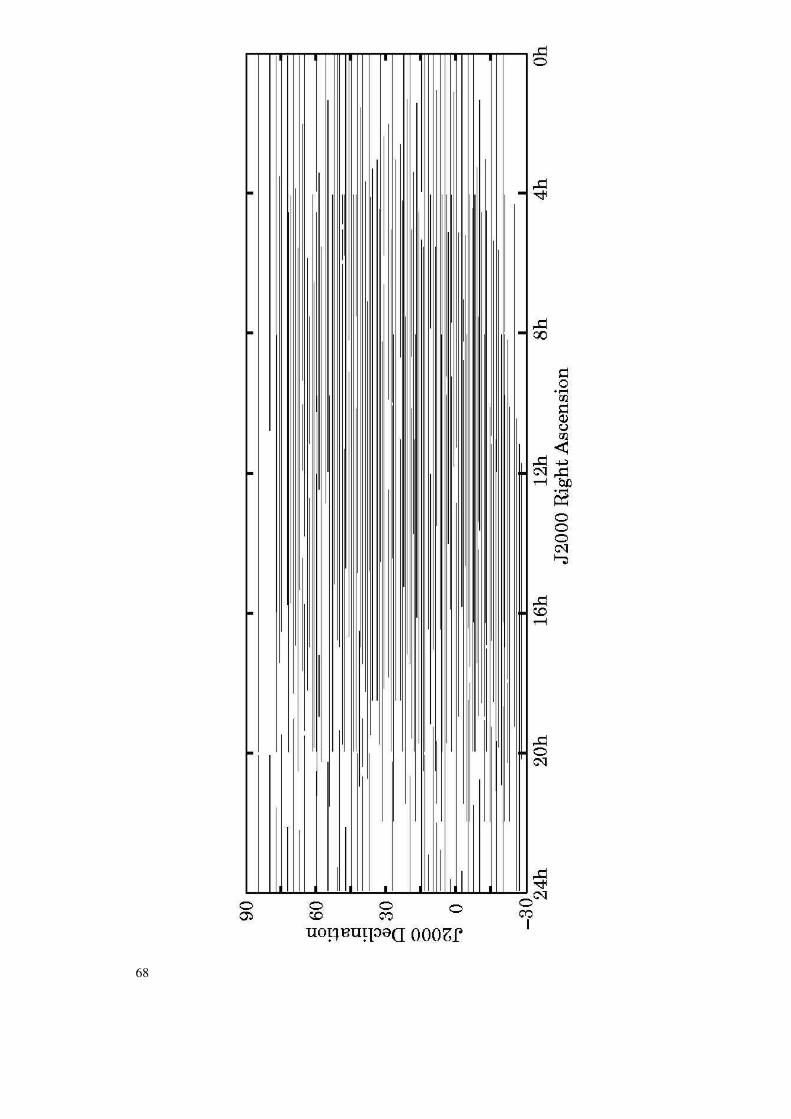
68
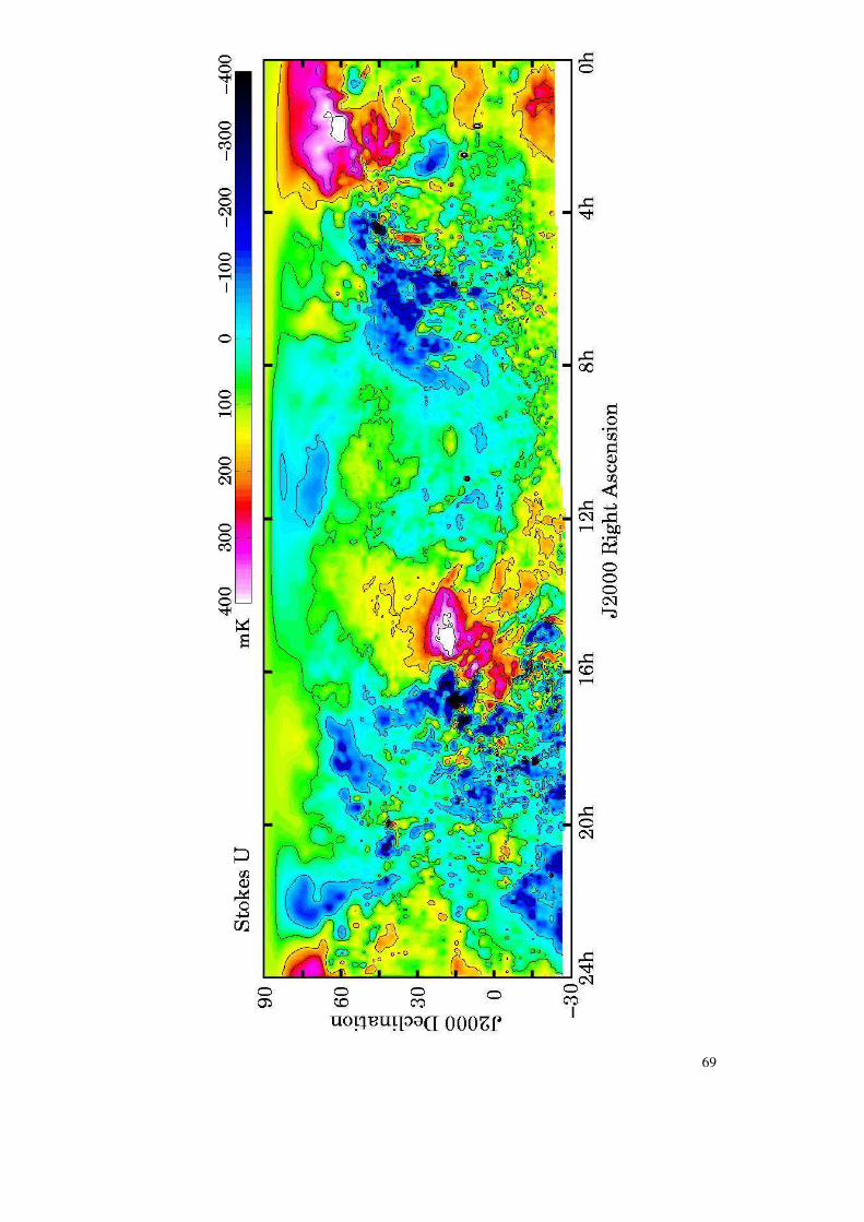
69
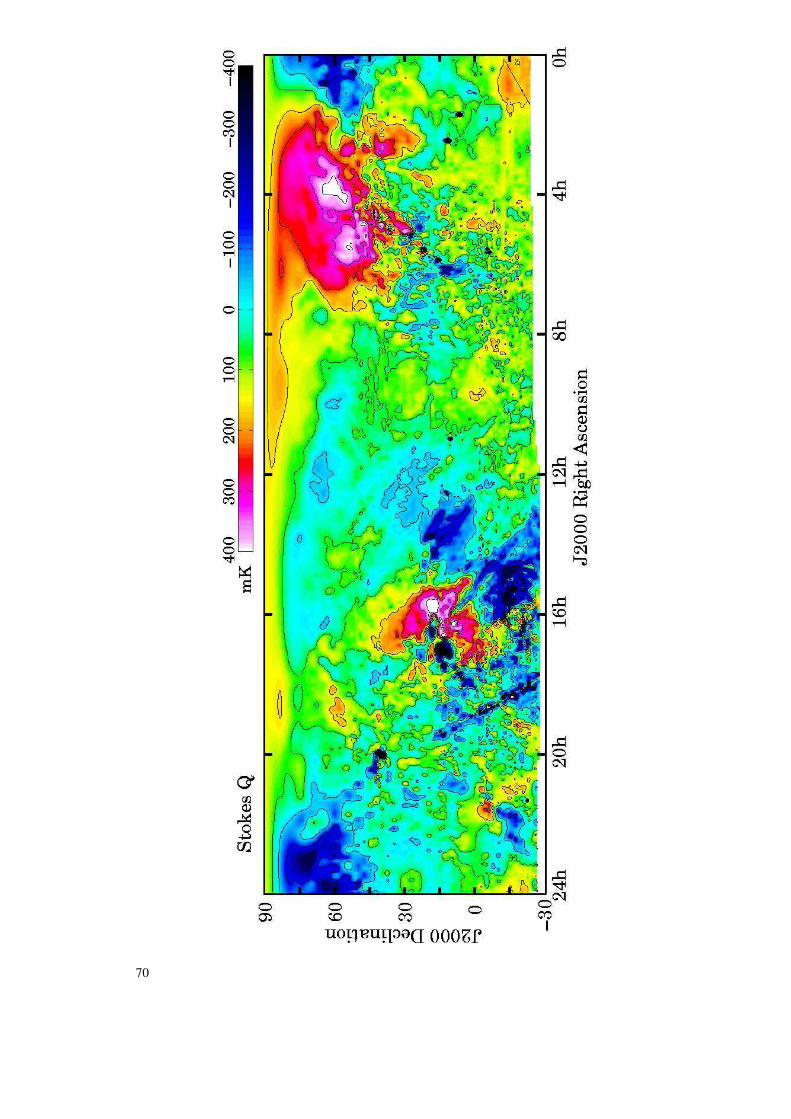
70
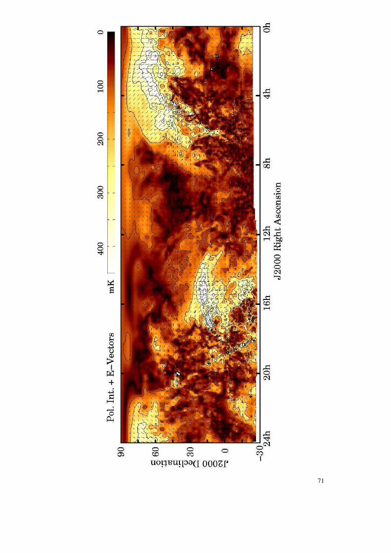
71
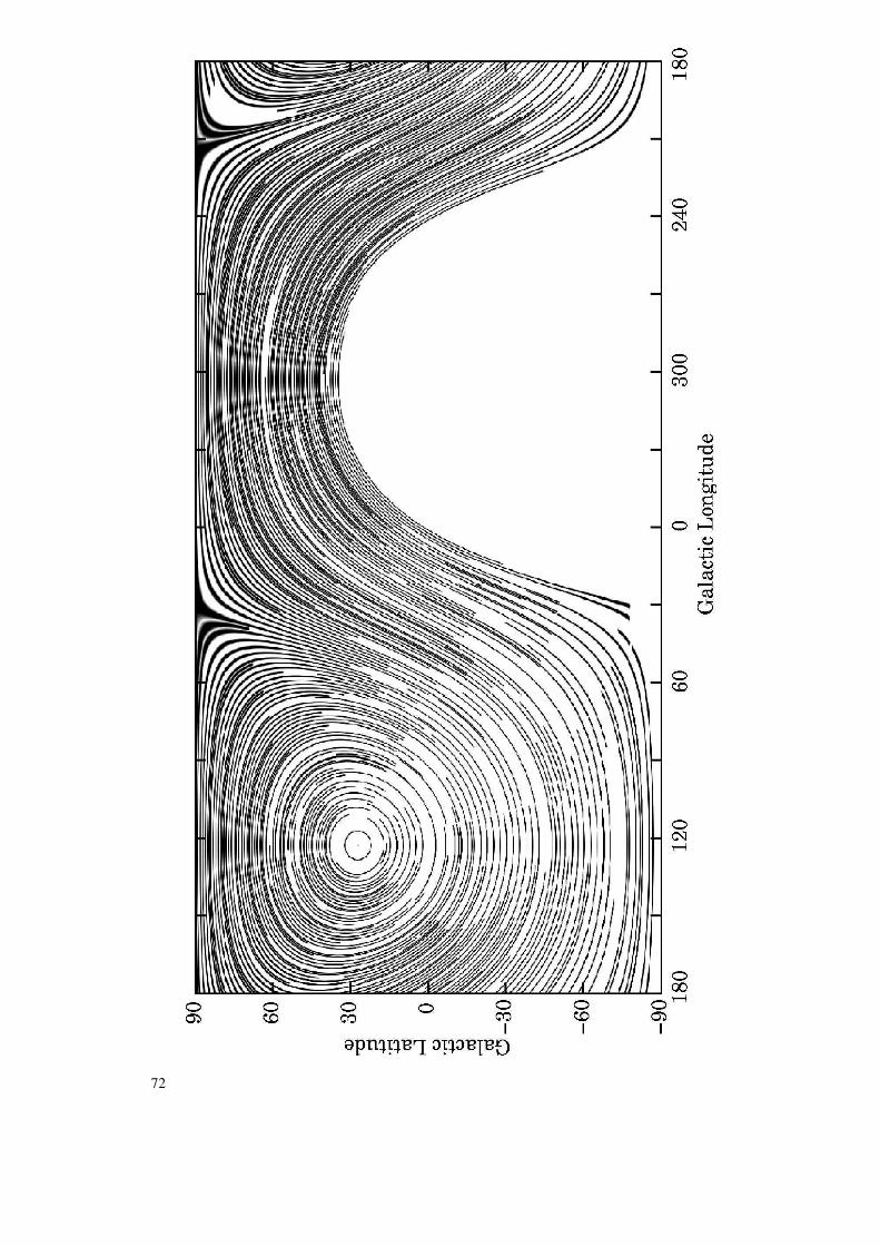
72
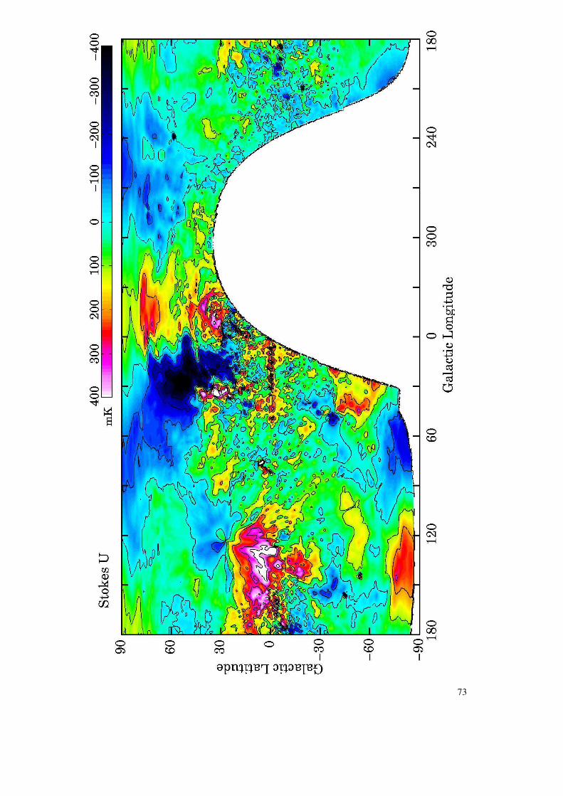
73
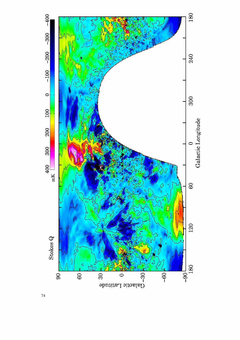
74
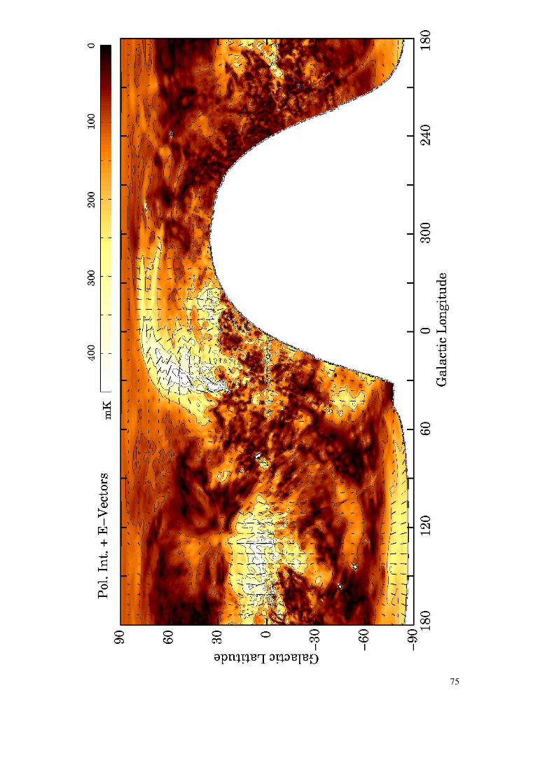
75
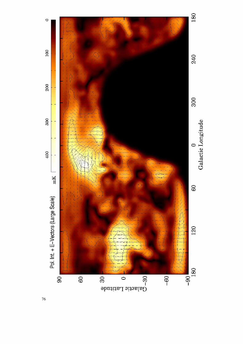
76
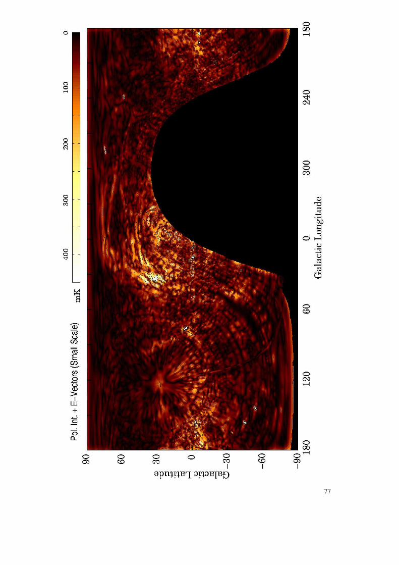
77
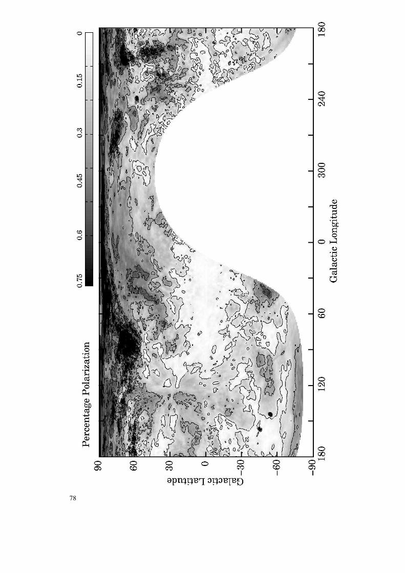
78

6 Improved Calibration of EffelsbergMedium Latitude Survey
In this chapter a preliminary map from the EMLS is absolutely calibrated using the 26-m Surveyas well as data from the LDS. The gain in resolution of the new survey compared to the LDS allowsa more accurate recovery of large-scale structures. This improves the quality of the calibration ofthe EMLS. In particular, high-resolution maps of polarized intensity and polarization angle showsignificant differences for different low-resolution data bases used for the absolute calibration.
6.1 Introduction
So far, the high-resolution polarimetric observations of the EMLS have been absolutely calibrated us-ing the low-resolution LDS. Missing offsets due to large-scale structure were determined by comparingStokes U and Q intensities of both surveys. In some areas surveyed by the EMLS it is possible to addmissing structures by computing difference maps between EMLS and LDS, which requires interpola-tion of the Dwingeloo data and smoothing of the EMLS maps. In some areas, however, the coarsesampling of the LDS does not allow an accurate interpolation. Here, only a tentative calibration byadjusting offset levels in U and Q maps could be achieved.
As discussed in Section 1.2 an adequate calibration of diffuse polarized emission is necessary for theanalysis. In the following the usability of the 26-m Survey for the absolute calibration of the EMLSis demonstrated using polarization maps of the Taurus, Auriga, and Perseus molecular cloud complex.The size of these maps is 40◦ × 16◦ in l × b. The final data are compared with tentatively calibratedmaps, which are corrected on the basis of only a few data points available from the LDS.
6.2 Method
For the absolute calibration of the EMLS a calibration scheme has been developed as described in Reichet al. (1990). This algorithm compares data of different angular resolution and corrects the large-scaleemission in the high-resolution data. The following steps of this method are most relevant here:
1. Convolution of the high-resolution map Ihighres (EMLS: 9.4′ beam size) to the angular resolutionof the low-resolution data Ilowres (Stockert, LDS: 36′ beam size):
I′highres = Ihighres ⊗ Gauss(36′ FWHM). (6.1)
In case of total intensity maps, a removal of strong point sources may be necessary prior toconvolution. Both surveys must be converted to the same temperature scale, e.g. main beambrightness temperature.
2. The difference map of the two data sets is added to the original high-resolution data:
I′′highres = Ilowres − I′highres + Ihighres (6.2)
79
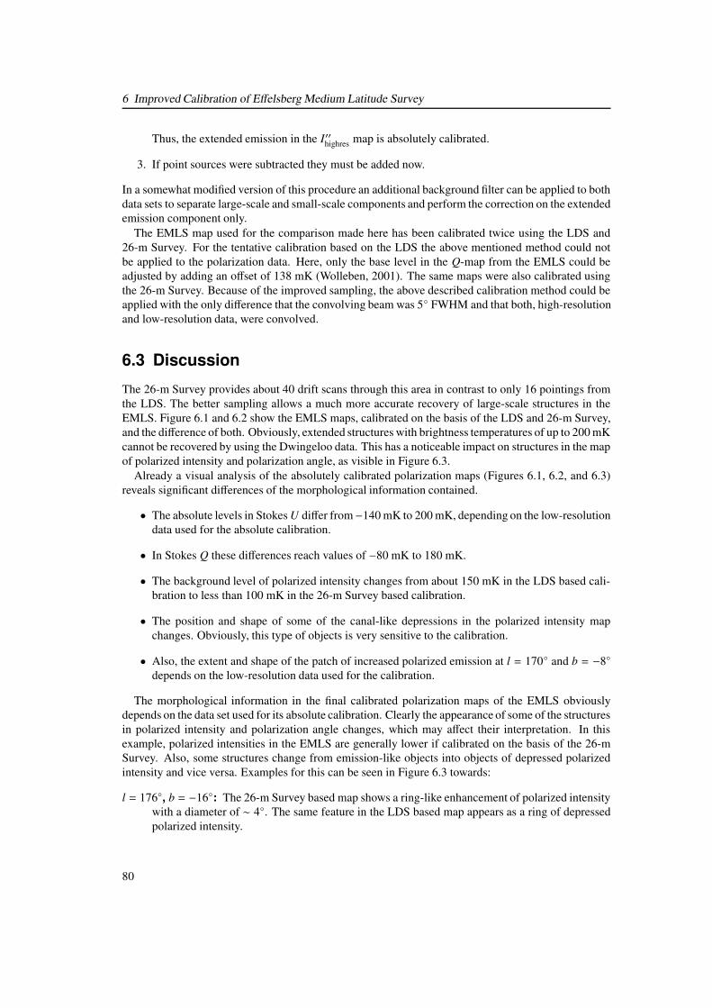
6 Improved Calibration of Effelsberg Medium Latitude Survey
Thus, the extended emission in the I′′highres map is absolutely calibrated.
3. If point sources were subtracted they must be added now.
In a somewhat modified version of this procedure an additional background filter can be applied to bothdata sets to separate large-scale and small-scale components and perform the correction on the extendedemission component only.
The EMLS map used for the comparison made here has been calibrated twice using the LDS and26-m Survey. For the tentative calibration based on the LDS the above mentioned method could notbe applied to the polarization data. Here, only the base level in the Q-map from the EMLS could beadjusted by adding an offset of 138 mK (Wolleben, 2001). The same maps were also calibrated usingthe 26-m Survey. Because of the improved sampling, the above described calibration method could beapplied with the only difference that the convolving beam was 5◦ FWHM and that both, high-resolutionand low-resolution data, were convolved.
6.3 Discussion
The 26-m Survey provides about 40 drift scans through this area in contrast to only 16 pointings fromthe LDS. The better sampling allows a much more accurate recovery of large-scale structures in theEMLS. Figure 6.1 and 6.2 show the EMLS maps, calibrated on the basis of the LDS and 26-m Survey,and the difference of both. Obviously, extended structures with brightness temperatures of up to 200 mKcannot be recovered by using the Dwingeloo data. This has a noticeable impact on structures in the mapof polarized intensity and polarization angle, as visible in Figure 6.3.
Already a visual analysis of the absolutely calibrated polarization maps (Figures 6.1, 6.2, and 6.3)reveals significant differences of the morphological information contained.
• The absolute levels in Stokes U differ from−140 mK to 200 mK, depending on the low-resolutiondata used for the absolute calibration.
• In Stokes Q these differences reach values of −80 mK to 180 mK.
• The background level of polarized intensity changes from about 150 mK in the LDS based cali-bration to less than 100 mK in the 26-m Survey based calibration.
• The position and shape of some of the canal-like depressions in the polarized intensity mapchanges. Obviously, this type of objects is very sensitive to the calibration.
• Also, the extent and shape of the patch of increased polarized emission at l = 170◦ and b = −8◦
depends on the low-resolution data used for the calibration.
The morphological information in the final calibrated polarization maps of the EMLS obviouslydepends on the data set used for its absolute calibration. Clearly the appearance of some of the structuresin polarized intensity and polarization angle changes, which may affect their interpretation. In thisexample, polarized intensities in the EMLS are generally lower if calibrated on the basis of the 26-mSurvey. Also, some structures change from emission-like objects into objects of depressed polarizedintensity and vice versa. Examples for this can be seen in Figure 6.3 towards:
l = 176◦, b = −16◦: The 26-m Survey based map shows a ring-like enhancement of polarized intensitywith a diameter of ∼ 4◦. The same feature in the LDS based map appears as a ring of depressedpolarized intensity.
80

6.3 Discussion
l = 184.◦5, b = −15◦: The LDS based map shows a polarized feature with a diameter of ∼ 2◦. Thisfeature almost completely vanishes in the 26-m Survey based map.
l = 177◦, b = −12◦: Pronounced canals of several degrees lengths are visible in the LDS based map.These canals disappear in the 26-m Survey based calibration.
These examples illustrate the importance of an accurate calibration of polarization data.
81
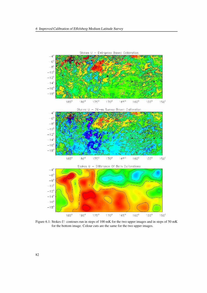
6 Improved Calibration of Effelsberg Medium Latitude Survey
Figure 6.1: Stokes U: contours run in steps of 100 mK for the two upper images and in steps of 50 mKfor the bottom image. Colour cuts are the same for the two upper images.
82
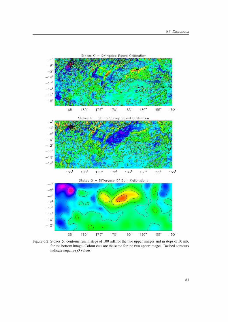
6.3 Discussion
Figure 6.2: Stokes Q: contours run in steps of 100 mK for the two upper images and in steps of 50 mKfor the bottom image. Colour cuts are the same for the two upper images. Dashed contoursindicate negative Q values.
83
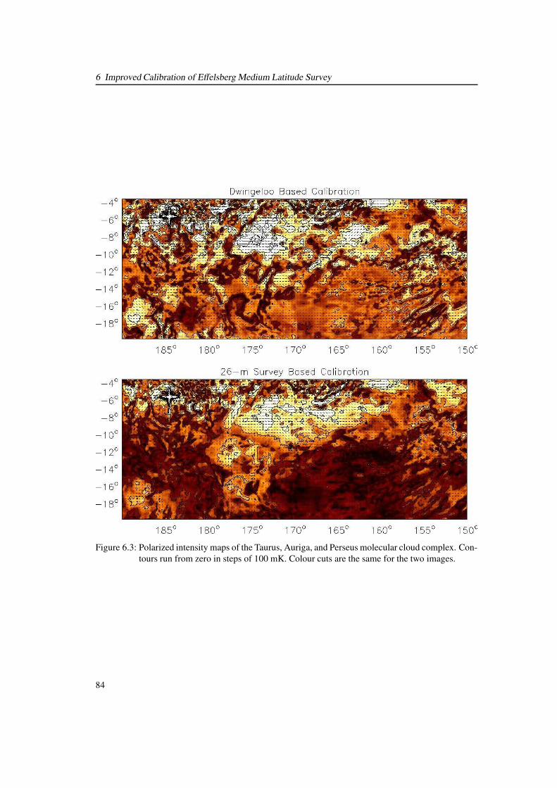
6 Improved Calibration of Effelsberg Medium Latitude Survey
Figure 6.3: Polarized intensity maps of the Taurus, Auriga, and Perseus molecular cloud complex. Con-tours run from zero in steps of 100 mK. Colour cuts are the same for the two images.
84
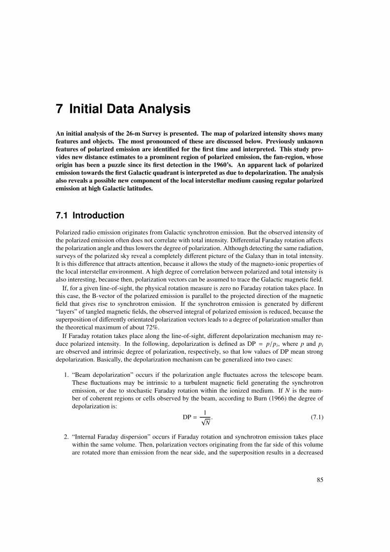
7 Initial Data Analysis
An initial analysis of the 26-m Survey is presented. The map of polarized intensity shows manyfeatures and objects. The most pronounced of these are discussed below. Previously unknownfeatures of polarized emission are identified for the first time and interpreted. This study pro-vides new distance estimates to a prominent region of polarized emission, the fan-region, whoseorigin has been a puzzle since its first detection in the 1960’s. An apparent lack of polarizedemission towards the first Galactic quadrant is interpreted as due to depolarization. The analysisalso reveals a possible new component of the local interstellar medium causing regular polarizedemission at high Galactic latitudes.
7.1 Introduction
Polarized radio emission originates from Galactic synchrotron emission. But the observed intensity ofthe polarized emission often does not correlate with total intensity. Differential Faraday rotation affectsthe polarization angle and thus lowers the degree of polarization. Although detecting the same radiation,surveys of the polarized sky reveal a completely different picture of the Galaxy than in total intensity.It is this difference that attracts attention, because it allows the study of the magneto-ionic properties ofthe local interstellar environment. A high degree of correlation between polarized and total intensity isalso interesting, because then, polarization vectors can be assumed to trace the Galactic magnetic field.
If, for a given line-of-sight, the physical rotation measure is zero no Faraday rotation takes place. Inthis case, the B-vector of the polarized emission is parallel to the projected direction of the magneticfield that gives rise to synchrotron emission. If the synchrotron emission is generated by different“layers” of tangled magnetic fields, the observed integral of polarized emission is reduced, because thesuperposition of differently orientated polarization vectors leads to a degree of polarization smaller thanthe theoretical maximum of about 72%.
If Faraday rotation takes place along the line-of-sight, different depolarization mechanism may re-duce polarized intensity. In the following, depolarization is defined as DP = p/pi, where p and pi
are observed and intrinsic degree of polarization, respectively, so that low values of DP mean strongdepolarization. Basically, the depolarization mechanism can be generalized into two cases:
1. “Beam depolarization” occurs if the polarization angle fluctuates across the telescope beam.These fluctuations may be intrinsic to a turbulent magnetic field generating the synchrotronemission, or due to stochastic Faraday rotation within the ionized medium. If N is the num-ber of coherent regions or cells observed by the beam, according to Burn (1966) the degree ofdepolarization is:
DP =1√
N. (7.1)
2. “Internal Faraday dispersion” occurs if Faraday rotation and synchrotron emission takes placewithin the same volume. Then, polarization vectors originating from the far side of this volumeare rotated more than emission from the near side, and the superposition results in a decreased
85
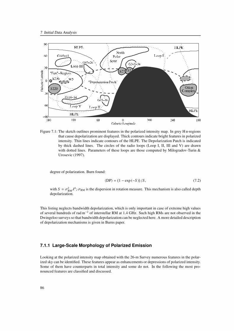
7 Initial Data Analysis
Figure 7.1: The sketch outlines prominent features in the polarized intensity map. In grey H -regionsthat cause depolarization are displayed. Thick contours indicate bright features in polarizedintensity. Thin lines indicate contours of the HLPE. The Depolarization Patch is indicatedby thick dashed lines. The circles of the radio loops (Loop I, II, III and V) are drawnwith dotted lines. Parameters of these loops are those computed by Milogradov-Turin &Urosevic (1997).
degree of polarization. Burn found:
〈DP〉 =(
1 − exp (−S ))
/S , (7.2)
with S = σ2RMλ
4; σRM is the dispersion in rotation measure. This mechanism is also called depthdepolarization.
This listing neglects bandwidth depolarization, which is only important in case of extreme high valuesof several hundreds of rad m−2 of interstellar RM at 1.4 GHz. Such high RMs are not observed in theDwingeloo surveys so that bandwidth depolarization can be neglected here. A more detailed descriptionof depolarization mechanisms is given in Burns paper.
7.1.1 Large-Scale Morphology of Polarized Emission
Looking at the polarized intensity map obtained with the 26-m Survey numerous features in the polar-ized sky can be identified. These features appear as enhancements or depressions of polarized intensity.Some of them have counterparts in total intensity and some do not. In the following the most pro-nounced features are classified and discussed.
86
7.1 Introduction
Enhanced Polarized Emission
A number of bright patches of polarized emission with intensities between 100 mK and 700 mK,exceeding the general “background” level1 of ∼ 60 mK, are visible in the polarized intensity map.The size of these features ranges from less than one degree up to several tens of degrees. Some canbe associated with known Galactic objects. At high Galactic latitudes, a previously unknown generalincrease of diffuse polarized intensity is noted: the so called “High Latitude Polarized Emission” (HLPEhereafter). The most pronounced objects, which are also outlined in Figure 7.1, are:
(a) The North-Polar Spur
A bright and spatially extended arc of polarized emission can be seen from l = 305◦ to l = 50◦, and b =30◦ to b = 80◦. Good correlation between polarized and total intensity is found. The new data reveal apreviously unseen filamentary structure in its polarized emission. The North-Polar Spur emission canbe associated with Loop I. Its percentage polarization is about 47% to 57%. See Section 7.2.1 for futherdiscussion.
(b) G343+34
This circular patch, about 15◦ in diameter, is located within the projected circle of Loop I. The averagepolarized intensity of this feature is about 300 mK with maximum intensities of about 450 mK. Thisstructure may be associated with the North-Polar Spur as its polarization angles follow the circularpattern of Loop I. To the south, the emission seems to be depolarized by the two H -regions S7 andS27. See Section 7.2.1 for futher discussion.
(c) The Fan-Region
The spatially extended polarized region of roughly 80◦ × 50◦ extent, centred at about l = 150◦ andb = 0◦ is commonly referred to as the “fan”-region. The percentage polarization towards this regionreaches values of 40%. The average polarization is about 26%. See Section 7.2.2 for futher discussion.
(d) High Latitude Polarized Emission
The 26-m Survey reveals an increase of polarized intensity towards the Galactic poles at latitudes|b| & 70◦. Polarized intensities rise from values of around 50 mK (60◦ < |b| < 70◦) to values of 110 mK(b > 70◦), and 230 mK (b < −70◦), respectively. The percentage polarization is ∼ 65% for the northerncomponent and 40% for the southern counterpart of the HLPE. See Section 7.3.3 for futher discussion.
(e) G45-46
Because of its positional coincidence and reasonable agreement of the B-vectors with the circle ofLoop II, the polarized intensity enhancement of about 200 mK over a region of about 15◦ in diameter,centred at l = 45 and b = −46◦, may be related to polarized emission from Loop II.
(f) G87+26
The feature at l = 87◦ and b = 26◦ with mean polarized intensity of about 160 mK seems to be part ofLoop III. The B-vectors of the polarized emission follow the corresponding circle.
1The background level of polarized intensity is determined at medium Galactic latitudes (40◦ . b . 70◦ and −70◦ . b . −40◦,respectively), excluding emission from bright polarized features.
87
7 Initial Data Analysis
(g) G116-54
The intensity and angle of polarized emission of this elongated feature at l = 116◦ and b = −54◦ arewell aligned with Loop V. The polarized intensity of this object is about 130 mK.
(h) G145+45
Because of the present incomplete sampling of the 26-m Survey at high declinations (& 80◦) the polar-ized feature at l = 145◦ and b = 45◦ seems to be distorted in the map. The polarized intensity is about110 mK and may be associated with Loop III.
Decreased Polarized Emission
Depressions in polarized intensity are observed toward a number of H -regions. The most obviousanticorrelations between Hα emission and polarized intensity are listed below, a more complete listis given in Table 7.1. The pronounced area of general low percentage polarization towards the firstquadrant of the Galaxy will be denoted as the “Depolarization Patch”.
(a) The Depolarization Patch
Very low percentage polarization around 3% over an elongated area towards the first quadrant of theGalaxy is observed in the 26-m Survey. The limits of the Depolarization Patch in Galactic latitude areremarkebly clear. At longitudes around l ≈ 0◦ the northern and southern boundaries of which are quitesymmetric at about |b| ≈ 30◦. At longitudes from ∼ 60◦ to ∼ 90◦ the latitude extent of the patch isless confined within |b| . 25◦. The limits in longitude are not as obvious. The patch seems to extendto longitude ∼ 100◦, covering an area of roughly 4000 square degrees on the northern sky. At aroundl ≈ 220◦, low percentage polarization at |b| . 20◦ suggests continuation of the Depolarization Patchinto the fourth quadrant. Although previous polarization surveys cover the region specified here, itsappearance as a coherent lack of polarization has never been noted.
(b) Sh2-7
The exciting star of the H -region S7 is δ Sco, which belongs to the Upper Scorpius association, theyoungest subgroup of the Scorpio-Centaurus OB association. The distance to this complex is 125 pc(de Geus & Burton, 1991). The average polarized intensity is 20 mK toward this object, while it is∼ 300 mK in its surrounding.
(c) Sh2-27
S27 is the H -region around the early-type star ζ Oph at a distance of about 170 pc (Fich et al., 1989).The average polarized intensity toward S27 is 30 mK and ∼ 250 mK in its surrounding.
(d) Sh2-199
This H -region is associated with W5. Altough this object is covered by only one drift scan of the26-m Survey the decrease of polarized emission is significant. This sets a lower limit to the distance ofthe fan region as discussed in Section 7.2.2.
88
7.1 Introduction
(e) Sh2-220
The California Nebula (S220) is a relatively large and close (∼ 400 pc) H -region located in the localspiral arm. The polarized intensity toward S220 is 40 mK, compared to ∼ 220 mK to the east and northof this object.
(f) Sh2-236
The H -region S236 is covered by four drift scans of the 26-m Survey, which show an anticorrelationbetween Hα emission and polarized intensity for this object. This anticorrelation can also been seen inthe EMLS (W. Reich, priv. comm.) strengthening evidence that this H -region is acting as a depolar-izing Faraday screen. As for S199 this sets a lower limit to the distance of the fan region. Toward S236the polarized intensity is 100 mK and it is ∼ 210 mK around it.
(g) Orion Complex
The Orion complex seems to act as a depolarizing screen, although it is not as obvious as for theother H -regions. The brightest objects of the Orion complex, such as M42, M43, Barnard’s Loop,and the Horsehead Nebula region, seemingly leave imprints in the background polarization structure.Additionally, some of the filamentary structure of the Orion complex up to b ≈ 0◦ obviously depolarizesbackground emission.
7.1.2 Local Interstellar Medium
Most of the objects visible in polarized intensity are strongly organized features of large angular extentsuggesting a rather local origin. Because of depolarization and Faraday rotation the diffuse polarizedemission is affected by the local ionized medium.
The region around the Sun within a radius of 150 to 200 pc is generally termed as the local interstellarmedium (LISM). The environment of the LISM is shaped by the influence of local objects such asLoop I or the close SCO-CEN stellar association (l = 330◦, b = +15◦, at 170 pc distance, Bertiau,1958). Part of the LISM is the Local Bubble, an elongated cavity, largely devoid of H with an averageradius of 100 pc. Because of the observation of an ultrasoft X-ray background, the local cavity isbelieved to be filled with hot plasma (e.g. Freyberg & Breitschwerdt, 2001). The Sun is embedded atthe inner edge of the Local Interstellar Cloud, a single entity within the Local Bubble.
The origin and evolution of the Local Bubble is still being discussed. Possible explanations proposea supernova remnant that has expanded to about 100 pc, or a recently heated superbubble produced byan already dissolved stellar association (see e.g. Cox & Reynolds, 1987).
Because of the spatial coincidence of the Local Bubble and Loop I, it is very likely that the two haveundergone some kind of interaction. Hydrodynamical computations show that a collision or merging ofthe two bubbles would leave a signature in the neutral hydrogen density. And, in fact, such an H -ringlocated roughly in the direction of the Galactic centre has been identified (Egger & Aschenbach, 1995).The distance to this ring and thus to the possible interaction region is 70 pc.
A number of radio spurs that can be joined into large circles on the sky are revealed by total intensitysurveys. A set of spurs belonging to the same hypothetical structure is named a “loop”. Four majorradio loops are generally recognized. These are Loop I (Large et al., 1962; Haslam et al., 1964),which has an intriguing filament called the North-Polar Spur, Loop II or Cetus arc (Large et al., 1962),Loop III or North-Celestial Pole Loop (Quigley & Haslam, 1965) and Loop IV (Large et al., 1966). Thegeometrical parameters of these loops were published by Berkhuijsen et al. (1971). Later, Milogradov-Turin & Urosevic (1997), who also proposed Loop V, used the continuum survey at 1420 MHz (Reich,1982; Reich & Reich, 1986) for a re-computation of the parameters. Their results agree well with the
89
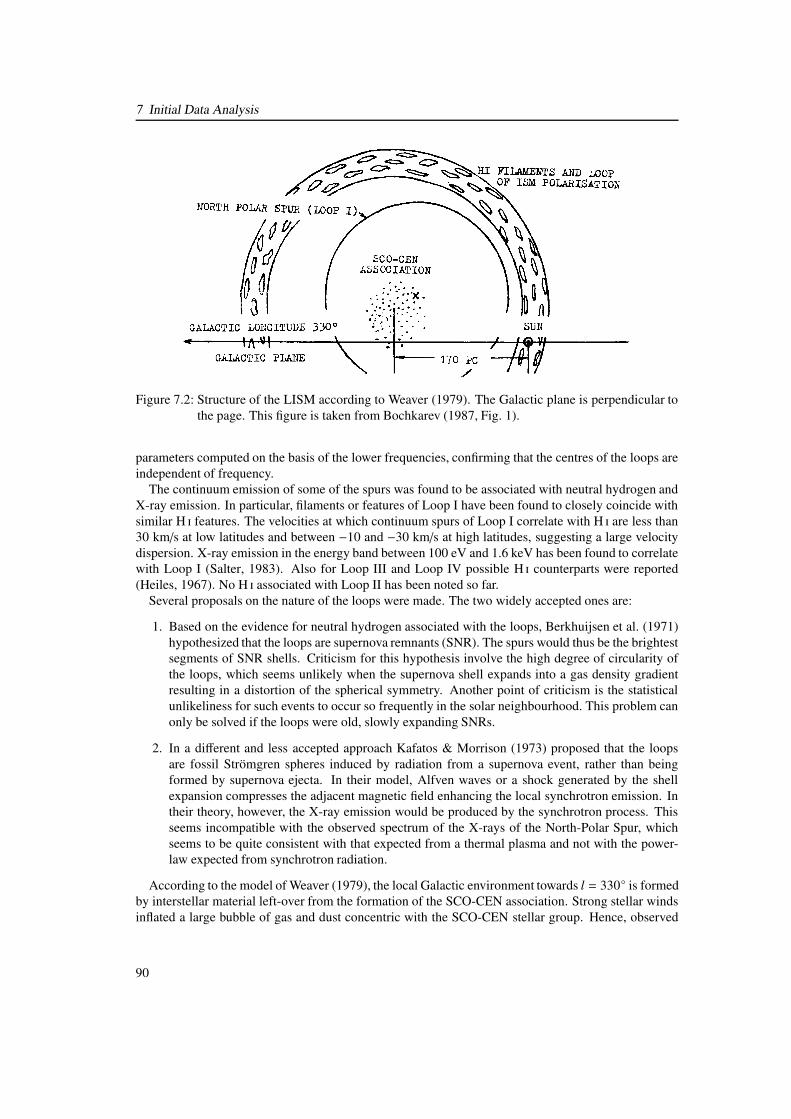
7 Initial Data Analysis
Figure 7.2: Structure of the LISM according to Weaver (1979). The Galactic plane is perpendicular tothe page. This figure is taken from Bochkarev (1987, Fig. 1).
parameters computed on the basis of the lower frequencies, confirming that the centres of the loops areindependent of frequency.
The continuum emission of some of the spurs was found to be associated with neutral hydrogen andX-ray emission. In particular, filaments or features of Loop I have been found to closely coincide withsimilar H features. The velocities at which continuum spurs of Loop I correlate with H are less than30 km/s at low latitudes and between −10 and −30 km/s at high latitudes, suggesting a large velocitydispersion. X-ray emission in the energy band between 100 eV and 1.6 keV has been found to correlatewith Loop I (Salter, 1983). Also for Loop III and Loop IV possible H counterparts were reported(Heiles, 1967). No H associated with Loop II has been noted so far.
Several proposals on the nature of the loops were made. The two widely accepted ones are:
1. Based on the evidence for neutral hydrogen associated with the loops, Berkhuijsen et al. (1971)hypothesized that the loops are supernova remnants (SNR). The spurs would thus be the brightestsegments of SNR shells. Criticism for this hypothesis involve the high degree of circularity ofthe loops, which seems unlikely when the supernova shell expands into a gas density gradientresulting in a distortion of the spherical symmetry. Another point of criticism is the statisticalunlikeliness for such events to occur so frequently in the solar neighbourhood. This problem canonly be solved if the loops were old, slowly expanding SNRs.
2. In a different and less accepted approach Kafatos & Morrison (1973) proposed that the loopsare fossil Strömgren spheres induced by radiation from a supernova event, rather than beingformed by supernova ejecta. In their model, Alfven waves or a shock generated by the shellexpansion compresses the adjacent magnetic field enhancing the local synchrotron emission. Intheir theory, however, the X-ray emission would be produced by the synchrotron process. Thisseems incompatible with the observed spectrum of the X-rays of the North-Polar Spur, whichseems to be quite consistent with that expected from a thermal plasma and not with the power-law expected from synchrotron radiation.
According to the model of Weaver (1979), the local Galactic environment towards l = 330◦ is formedby interstellar material left-over from the formation of the SCO-CEN association. Strong stellar windsinflated a large bubble of gas and dust concentric with the SCO-CEN stellar group. Hence, observed
90
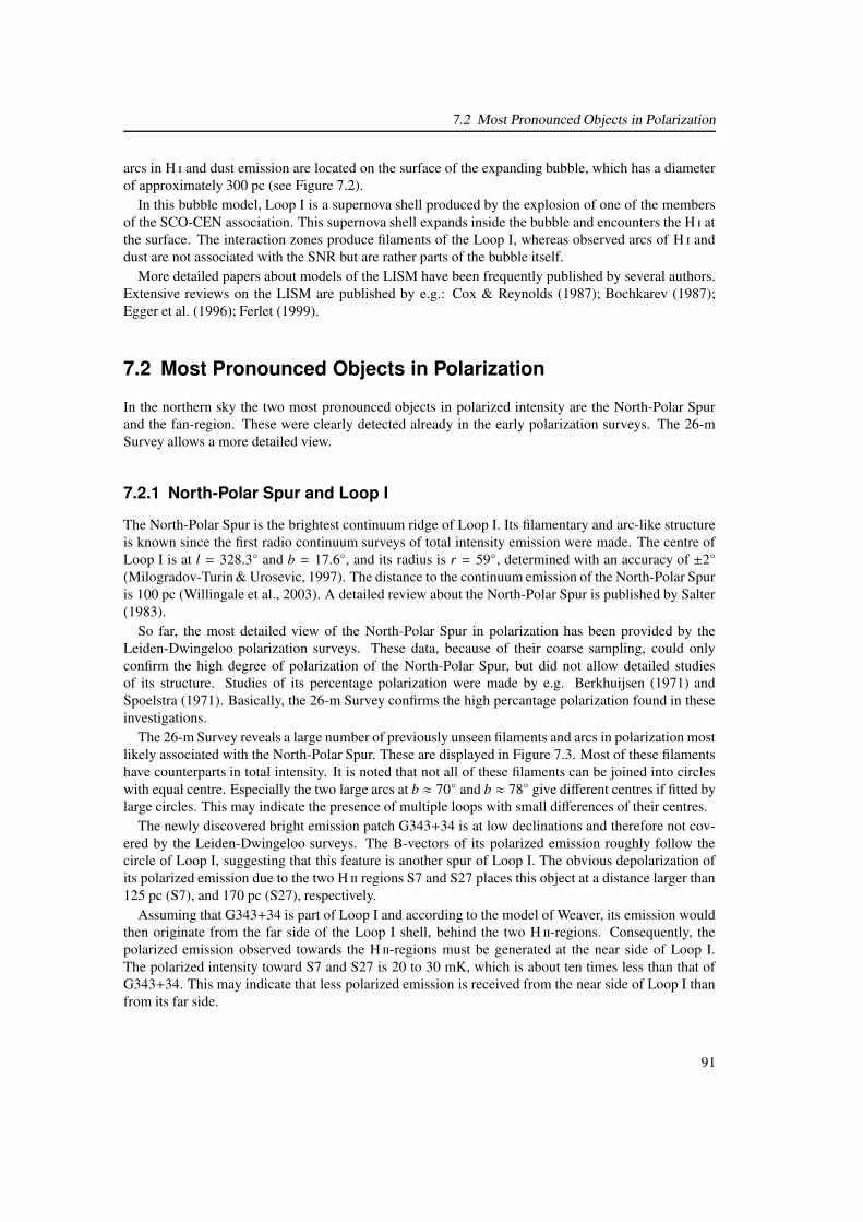
7.2 Most Pronounced Objects in Polarization
arcs in H and dust emission are located on the surface of the expanding bubble, which has a diameterof approximately 300 pc (see Figure 7.2).
In this bubble model, Loop I is a supernova shell produced by the explosion of one of the membersof the SCO-CEN association. This supernova shell expands inside the bubble and encounters the H atthe surface. The interaction zones produce filaments of the Loop I, whereas observed arcs of H anddust are not associated with the SNR but are rather parts of the bubble itself.
More detailed papers about models of the LISM have been frequently published by several authors.Extensive reviews on the LISM are published by e.g.: Cox & Reynolds (1987); Bochkarev (1987);Egger et al. (1996); Ferlet (1999).
7.2 Most Pronounced Objects in Polarization
In the northern sky the two most pronounced objects in polarized intensity are the North-Polar Spurand the fan-region. These were clearly detected already in the early polarization surveys. The 26-mSurvey allows a more detailed view.
7.2.1 North-Polar Spur and Loop I
The North-Polar Spur is the brightest continuum ridge of Loop I. Its filamentary and arc-like structureis known since the first radio continuum surveys of total intensity emission were made. The centre ofLoop I is at l = 328.3◦ and b = 17.6◦, and its radius is r = 59◦, determined with an accuracy of ±2◦
(Milogradov-Turin & Urosevic, 1997). The distance to the continuum emission of the North-Polar Spuris 100 pc (Willingale et al., 2003). A detailed review about the North-Polar Spur is published by Salter(1983).
So far, the most detailed view of the North-Polar Spur in polarization has been provided by theLeiden-Dwingeloo polarization surveys. These data, because of their coarse sampling, could onlyconfirm the high degree of polarization of the North-Polar Spur, but did not allow detailed studiesof its structure. Studies of its percentage polarization were made by e.g. Berkhuijsen (1971) andSpoelstra (1971). Basically, the 26-m Survey confirms the high percantage polarization found in theseinvestigations.
The 26-m Survey reveals a large number of previously unseen filaments and arcs in polarization mostlikely associated with the North-Polar Spur. These are displayed in Figure 7.3. Most of these filamentshave counterparts in total intensity. It is noted that not all of these filaments can be joined into circleswith equal centre. Especially the two large arcs at b ≈ 70◦ and b ≈ 78◦ give different centres if fitted bylarge circles. This may indicate the presence of multiple loops with small differences of their centres.
The newly discovered bright emission patch G343+34 is at low declinations and therefore not cov-ered by the Leiden-Dwingeloo surveys. The B-vectors of its polarized emission roughly follow thecircle of Loop I, suggesting that this feature is another spur of Loop I. The obvious depolarization ofits polarized emission due to the two H regions S7 and S27 places this object at a distance larger than125 pc (S7), and 170 pc (S27), respectively.
Assuming that G343+34 is part of Loop I and according to the model of Weaver, its emission wouldthen originate from the far side of the Loop I shell, behind the two H -regions. Consequently, thepolarized emission observed towards the H -regions must be generated at the near side of Loop I.The polarized intensity toward S7 and S27 is 20 to 30 mK, which is about ten times less than that ofG343+34. This may indicate that less polarized emission is received from the near side of Loop I thanfrom its far side.
91

7 Initial Data Analysis
� �� �� �� �
� �� �� �� �
� � � � � � � � � � � � � �� � � � � � � � � � � � � �� � � � � � � � � � � � � �� � � � � � � � � � � � � �� � � � � � � � � � � � � �� � � � � � � � � � � � � �� � � � � � � � � � � � � �� � � � � � � � � � � � � �� � � � � � � � � � � � � �� � � � � � � � � � � � � �
� � � � � � � � � � � � �� � � � � � � � � � � � �� � � � � � � � � � � � �� � � � � � � � � � � � �� � � � � � � � � � � � �� � � � � � � � � � � � �� � � � � � � � � � � � �� � � � � � � � � � � � �� � � � � � � � � � � � �� � � � � � � � � � � � �HII
DIFFUSE
S7S27
� � � � � � � � � � �� � � � � � � � � � �� � � � � � � � � � �� � � � � � � � � � �� � � �� � �
� �
�
� �
�� ��
��
� �� �
� ��
��
����
����
� ��
60 40 20 0 300340320 260280
80
60
40
20
0
Lat
itude
Longitude
Figure 7.3: Sketch highlighting the filaments of the North-Polar Spur with B-vectors of polarized emis-sion at 1.4 GHz overlayed. The shadowed areas are regions of enhanced Hα emission.Vectors of equal length are shown for PI ≥ 140 mK. Solid lines mark contours of filamentsin the polarized intensity map, whereas dashed lines indicate less confined filaments.
7.2.2 The Fan-Region
The fan-region is an extended area with strong polarized intensity and high percentage polarization. Itscentre is commonly quoted at l = 140◦ and b = 5◦. The increase in sensitivity and sampling of the26-m Survey, however, reveals a larger extent of the fan-region then previously believed. Therefore, arevised size and position is claimed. If the centre of the whole structure is taken, instead of the locationof the maximum of polarized intensity, the centre is roughly at l = 150◦ and b = 0◦. The spatial extentis several tens of degrees in diameter, covering an area of about 4000 square degrees.
The high degree of polarization towards the fan-region was noted by Westerhout et al. (1962) andBrouw et al. (1962) who used the Dwingeloo-telescope at 408 MHz. Measurements of Wielebinskiet al. (1962), made at Cambridge at the same frequency, and Razin et al. (1968)) at Staryi Pustyn at437 MHz, 510 MHz, and 735 MHz comfirmed these results. The 26-m Survey also clearly shows that,at 1410 MHz, the fan-region is one of the two brightest polarized patches in the northern sky withpolarized intensities of up to 500 mK.
The E-vectors of the polarized emission of the fan-region are highly ordered and perpendicular to theGalactic plane, indicating a magnetic field parallel to the plane. A comparison of radio polarization datawith optical data confirms that the strong polarized emission may be due to a magnetic field parallelto the Galactic plane and perpendicular to the line-of-sight towards l = 140◦ (Berkhuijsen et al., 1964;Bingham & Shakeshaft, 1967). This is in agreement with low Faraday rotation observed in this area(Spoelstra, 1984).
A constraint for the distance to the fan-region on the basis of starlight polarization was suggestedby Spoelstra (1984). He concluded that the polarized emission must come from distances within about450 pc and thus traces very local synchrotron radiation.
92

7.2 Most Pronounced Objects in Polarization
Figure 7.4: Depolarization at the southern edge of the emission feature G343+34 caused by the twoH -regions S27 (left) and S7 (right). The map shows polarized intensity (26m-Survey)with contours of Hα emission (Finkbeiner, 2003) overlayed.
Morphological studies of the fan region have been fairly limited because of the sparse sampling ofthe early polarization surveys. Reasonably sampled data of the fan region at 408 MHz were analyzedby Verschuur (1968) and Wilkinson & Smith (1974) who studied the depolarizing effects of H -regionslocated towards the fan-region.
Verschuur found a ring-like structure of low polarized intensity at 408 MHz towards l = 137.◦4and b = 7.◦1, which he interpreted as due to depolarization or Faraday rotation. He suggested thatenhanced RM is caused by a magneto-ionized medium associated with the Strömgren sphere aroundthe B2 star HD 20336 and causing depolarization. Its position, in fact, coincides with the centre of thedepolarization ring. The distance to HD 20336 is 140 to 200 pc (see references in Verschuur, 1968).Rubin et al. (1962) give a distance of 400 pc to this star. Verschuur concluded that most polarizedradiation must originate from distances larger than that of HD 20336.
Wilkinson and Smith looked at a number of H -regions that should show similar effects like the B2star HD 20336. They did not find such effects towards the H -regions S202, S185, S205 and S216.From the absence of depolarization they concluded that most polarized radiation towards the fan regionoriginates within a distance of about 500 pc (±200 pc).
These two studies and the investigation of RMs made by Spoelstra suggested a distance to the fan-region of less then 500 pc and more then about 200 pc. According to these results the fan-region isa layer of enhanced polarized emission, which could be due to enhanced synchrotron emissivity anda particular regular magnetic field perpendicular to the line-of-sight causing only little depolarizationcompared with other directions. Based on the new data from the 26-m Survey the distance to the fan-region can be revised, because depolarization observable towards a number of H -regions reveals alarger distance to this object. This is discussed in the following.
93
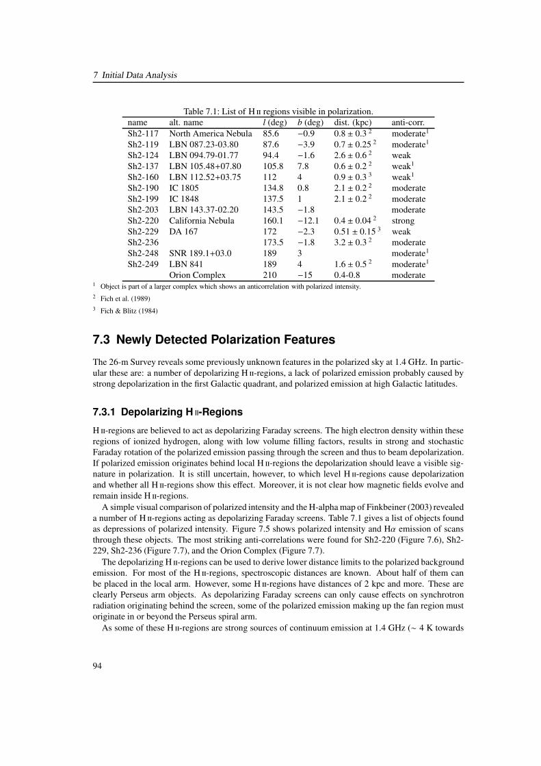
7 Initial Data Analysis
Table 7.1: List of H regions visible in polarization.name alt. name l (deg) b (deg) dist. (kpc) anti-corr.Sh2-117 North America Nebula 85.6 −0.9 0.8 ± 0.3 2 moderate1
Sh2-119 LBN 087.23-03.80 87.6 −3.9 0.7 ± 0.25 2 moderate1
Sh2-124 LBN 094.79-01.77 94.4 −1.6 2.6 ± 0.6 2 weakSh2-137 LBN 105.48+07.80 105.8 7.8 0.6 ± 0.2 2 weak1
Sh2-160 LBN 112.52+03.75 112 4 0.9 ± 0.3 3 weak1
Sh2-190 IC 1805 134.8 0.8 2.1 ± 0.2 2 moderateSh2-199 IC 1848 137.5 1 2.1 ± 0.2 2 moderateSh2-203 LBN 143.37-02.20 143.5 −1.8 moderateSh2-220 California Nebula 160.1 −12.1 0.4 ± 0.04 2 strongSh2-229 DA 167 172 −2.3 0.51 ± 0.15 3 weakSh2-236 173.5 −1.8 3.2 ± 0.3 2 moderateSh2-248 SNR 189.1+03.0 189 3 moderate1
Sh2-249 LBN 841 189 4 1.6 ± 0.5 2 moderate1
Orion Complex 210 −15 0.4-0.8 moderate1 Object is part of a larger complex which shows an anticorrelation with polarized intensity.2 Fich et al. (1989)3 Fich & Blitz (1984)
7.3 Newly Detected Polarization Features
The 26-m Survey reveals some previously unknown features in the polarized sky at 1.4 GHz. In partic-ular these are: a number of depolarizing H -regions, a lack of polarized emission probably caused bystrong depolarization in the first Galactic quadrant, and polarized emission at high Galactic latitudes.
7.3.1 Depolarizing H -Regions
H -regions are believed to act as depolarizing Faraday screens. The high electron density within theseregions of ionized hydrogen, along with low volume filling factors, results in strong and stochasticFaraday rotation of the polarized emission passing through the screen and thus to beam depolarization.If polarized emission originates behind local H -regions the depolarization should leave a visible sig-nature in polarization. It is still uncertain, however, to which level H -regions cause depolarizationand whether all H -regions show this effect. Moreover, it is not clear how magnetic fields evolve andremain inside H -regions.
A simple visual comparison of polarized intensity and the H-alpha map of Finkbeiner (2003) revealeda number of H -regions acting as depolarizing Faraday screens. Table 7.1 gives a list of objects foundas depressions of polarized intensity. Figure 7.5 shows polarized intensity and Hα emission of scansthrough these objects. The most striking anti-correlations were found for Sh2-220 (Figure 7.6), Sh2-229, Sh2-236 (Figure 7.7), and the Orion Complex (Figure 7.7).
The depolarizing H -regions can be used to derive lower distance limits to the polarized backgroundemission. For most of the H -regions, spectroscopic distances are known. About half of them canbe placed in the local arm. However, some H -regions have distances of 2 kpc and more. These areclearly Perseus arm objects. As depolarizing Faraday screens can only cause effects on synchrotronradiation originating behind the screen, some of the polarized emission making up the fan region mustoriginate in or beyond the Perseus spiral arm.
As some of these H -regions are strong sources of continuum emission at 1.4 GHz (∼ 4 K towards
94
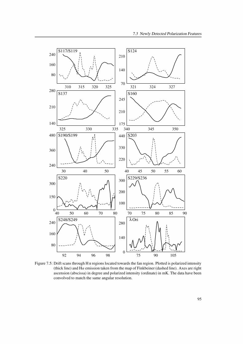
7.3 Newly Detected Polarization Features
310 315 320 325
80
160
240
321 324 32770
140
210
325 330 335140
210
280
340 345 350175
210
245
30 40 50240
360
480
40 45 50 55 60
220
330
440
40 50 60 70 800
150
300
70 75 80 85 90
100
200
300
92 94 96 98
80
160
240
75 90 1050
140
280
� � � �� � � �� � � �! ! !! ! !! ! !
" " " " "" " " " "" " " " "# # # # ## # # # ## # # # #
$ $ $ $ $$ $ $ $ $$ $ $ $ $% % % % %% % % % %% % % % %
& & & & & && & & & & &' ' ' ' '' ' ' ' '
S117/S119 S124
S137 S160
S190/S199 S203
S220 S229/S236
S248/S249 Oriλ
Figure 7.5: Drift scans through H regions located towards the fan region. Plotted is polarized intensity(thick line) and Hα emission taken from the map of Finkbeiner (dashed line). Axes are rightascension (abscissa) in degree and polarized intensity (ordinate) in mK. The data have beenconvolved to match the same angular resolution.
95
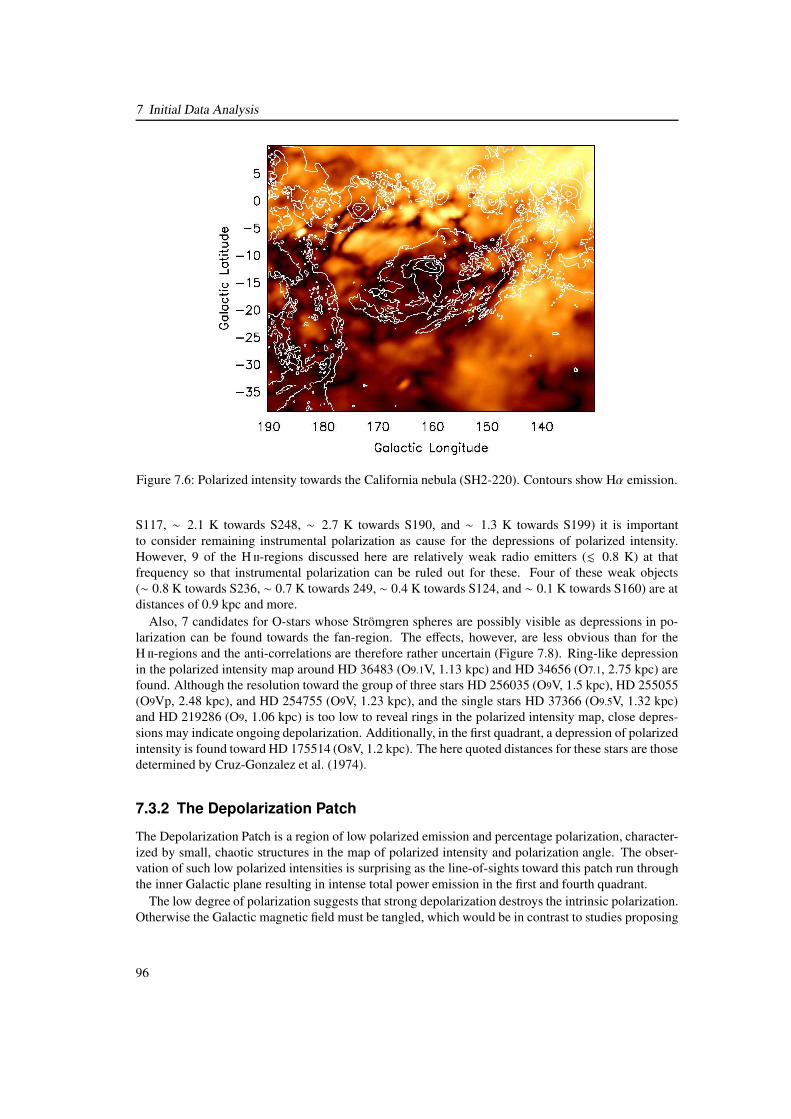
7 Initial Data Analysis
Figure 7.6: Polarized intensity towards the California nebula (SH2-220). Contours show Hα emission.
S117, ∼ 2.1 K towards S248, ∼ 2.7 K towards S190, and ∼ 1.3 K towards S199) it is importantto consider remaining instrumental polarization as cause for the depressions of polarized intensity.However, 9 of the H -regions discussed here are relatively weak radio emitters (. 0.8 K) at thatfrequency so that instrumental polarization can be ruled out for these. Four of these weak objects(∼ 0.8 K towards S236, ∼ 0.7 K towards 249, ∼ 0.4 K towards S124, and ∼ 0.1 K towards S160) are atdistances of 0.9 kpc and more.
Also, 7 candidates for O-stars whose Strömgren spheres are possibly visible as depressions in po-larization can be found towards the fan-region. The effects, however, are less obvious than for theH -regions and the anti-correlations are therefore rather uncertain (Figure 7.8). Ring-like depressionin the polarized intensity map around HD 36483 (O9.1V, 1.13 kpc) and HD 34656 (O7.1, 2.75 kpc) arefound. Although the resolution toward the group of three stars HD 256035 (O9V, 1.5 kpc), HD 255055(O9Vp, 2.48 kpc), and HD 254755 (O9V, 1.23 kpc), and the single stars HD 37366 (O9.5V, 1.32 kpc)and HD 219286 (O9, 1.06 kpc) is too low to reveal rings in the polarized intensity map, close depres-sions may indicate ongoing depolarization. Additionally, in the first quadrant, a depression of polarizedintensity is found toward HD 175514 (O8V, 1.2 kpc). The here quoted distances for these stars are thosedetermined by Cruz-Gonzalez et al. (1974).
7.3.2 The Depolarization Patch
The Depolarization Patch is a region of low polarized emission and percentage polarization, character-ized by small, chaotic structures in the map of polarized intensity and polarization angle. The obser-vation of such low polarized intensities is surprising as the line-of-sights toward this patch run throughthe inner Galactic plane resulting in intense total power emission in the first and fourth quadrant.
The low degree of polarization suggests that strong depolarization destroys the intrinsic polarization.Otherwise the Galactic magnetic field must be tangled, which would be in contrast to studies proposing
96
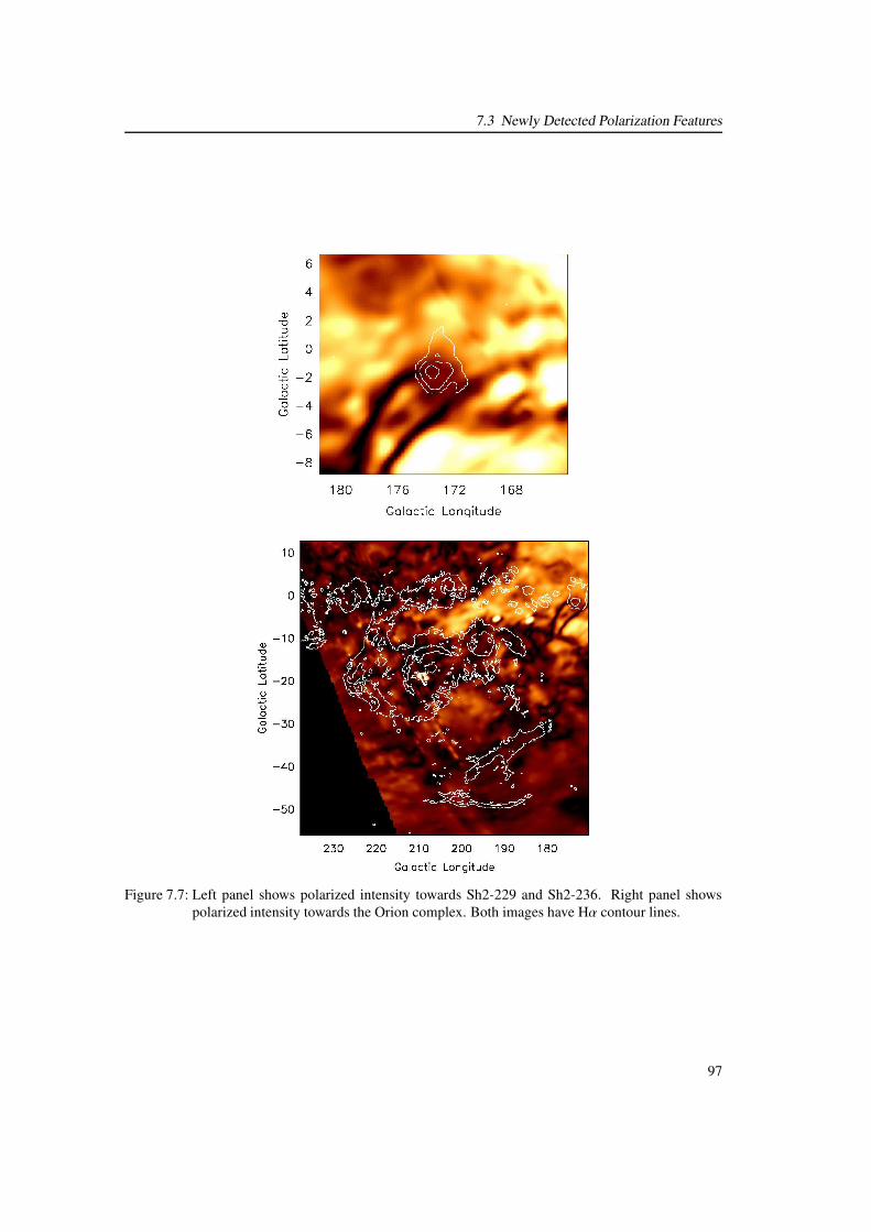
7.3 Newly Detected Polarization Features
Figure 7.7: Left panel shows polarized intensity towards Sh2-229 and Sh2-236. Right panel showspolarized intensity towards the Orion complex. Both images have Hα contour lines.
97
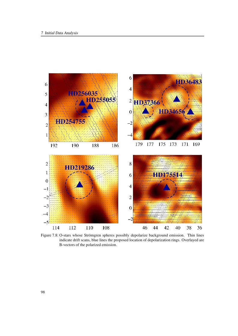
7 Initial Data Analysis
Figure 7.8: O-stars whose Strömgren spheres possibly depolarize background emission. Thin linesindicate drift scans, blue lines the proposed location of depolarization rings. Overlayed areB-vectors of the polarized emission.
98
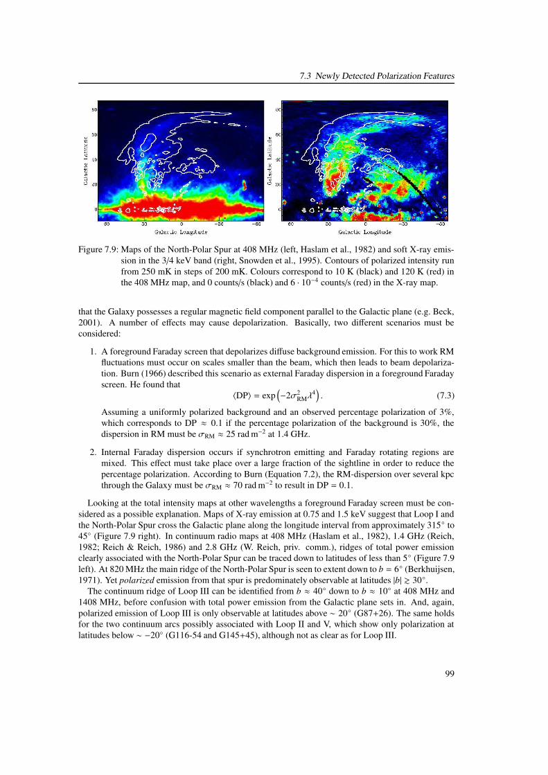
7.3 Newly Detected Polarization Features
Figure 7.9: Maps of the North-Polar Spur at 408 MHz (left, Haslam et al., 1982) and soft X-ray emis-sion in the 3/4 keV band (right, Snowden et al., 1995). Contours of polarized intensity runfrom 250 mK in steps of 200 mK. Colours correspond to 10 K (black) and 120 K (red) inthe 408 MHz map, and 0 counts/s (black) and 6 · 10−4 counts/s (red) in the X-ray map.
that the Galaxy possesses a regular magnetic field component parallel to the Galactic plane (e.g. Beck,2001). A number of effects may cause depolarization. Basically, two different scenarios must beconsidered:
1. A foreground Faraday screen that depolarizes diffuse background emission. For this to work RMfluctuations must occur on scales smaller than the beam, which then leads to beam depolariza-tion. Burn (1966) described this scenario as external Faraday dispersion in a foreground Faradayscreen. He found that
〈DP〉 = exp(
−2σ2RMλ
4)
. (7.3)
Assuming a uniformly polarized background and an observed percentage polarization of 3%,which corresponds to DP ≈ 0.1 if the percentage polarization of the background is 30%, thedispersion in RM must be σRM ≈ 25 rad m−2 at 1.4 GHz.
2. Internal Faraday dispersion occurs if synchrotron emitting and Faraday rotating regions aremixed. This effect must take place over a large fraction of the sightline in order to reduce thepercentage polarization. According to Burn (Equation 7.2), the RM-dispersion over several kpcthrough the Galaxy must be σRM ≈ 70 rad m−2 to result in DP = 0.1.
Looking at the total intensity maps at other wavelengths a foreground Faraday screen must be con-sidered as a possible explanation. Maps of X-ray emission at 0.75 and 1.5 keV suggest that Loop I andthe North-Polar Spur cross the Galactic plane along the longitude interval from approximately 315◦ to45◦ (Figure 7.9 right). In continuum radio maps at 408 MHz (Haslam et al., 1982), 1.4 GHz (Reich,1982; Reich & Reich, 1986) and 2.8 GHz (W. Reich, priv. comm.), ridges of total power emissionclearly associated with the North-Polar Spur can be traced down to latitudes of less than 5◦ (Figure 7.9left). At 820 MHz the main ridge of the North-Polar Spur is seen to extent down to b = 6◦ (Berkhuijsen,1971). Yet polarized emission from that spur is predominately observable at latitudes |b| & 30◦.
The continuum ridge of Loop III can be identified from b ≈ 40◦ down to b ≈ 10◦ at 408 MHz and1408 MHz, before confusion with total power emission from the Galactic plane sets in. And, again,polarized emission of Loop III is only observable at latitudes above ∼ 20◦ (G87+26). The same holdsfor the two continuum arcs possibly associated with Loop II and V, which show only polarization atlatitudes below ∼ −20◦ (G116-54 and G145+45), although not as clear as for Loop III.
99

7 Initial Data Analysis
Assuming that the radio loops are intrinsically polarized even at low Galactic latitudes and that theirpolarization is observable with the 26-m Telescope, strong depolarization must occur between the Sunand Loop I, II, III, and V, in the area of the Depolarization Patch. The distances to these radio loops arecommonly assumed between 100 pc (Loop I) and a few hundred parsecs (Loop III and V). Based onthe observation that these radio loops are unpolarized within ±20◦ to ±30◦ latitude, the existence of anearby depolarizing Faraday screen seems possible. This Faraday screen must depolarize the Galacticsynchrotron emission of the entire first and possibly fourth quadrant in the 26-m Survey.
Such a Faraday screen causes significant depolarization only if the distribution of Faraday rotationinduced by the cells is wide enough. A plausible number for the width of the RM distribution is σRM ≈35 rad m−2, which causes Faraday rotation of about ±90◦ at 1.4 GHz and hence high depolarization ofa uniformly polarized background for a cell number N > 1.
Limits on the electron density of the proposed Faraday screen can be derived from the full-sky H-alpha map of Finkbeiner (2003). A comparison of this map with polarized intensity shows that the2 Rayleigh contour line of Hα emission borders well the Depolarization Patch to Galactic north andsouth. Taking this as an upper limit for the thermal emissivity of the screen, the lower limit of theelectron density calculates to:
ne(screen) =
√
EML≈√
1 RayleighL
, (7.4)
with 1 Rayleigh corresponding to an emission measure of EM = 2 pc cm−6. To produce RMs of35 rad m−2, a magnetic field of B‖ ≈ 40 µG for a thickness of 1 pc, B‖ ≈ 13 µG for a thickness of 10 pc,or B‖ ≈ 9 µG for a thickness of 20 pc of the screen is required. Then, the electron densities within thescreen must be: 1.1 cm−3, 0.3 cm−3, or 0.2 cm−3, respectively.
Against this model speaks the high symmetry of the Depolarization Patch about the Galactic plane,which may indicate a relation to the Galactic electron distribution rather than a local origin. The de-polarization would then be caused by depth depolarization with the sharp boundaries reflecting thez-distribution of the magneto-ionic medium causing depolarization. In this scenario, the observed syn-chrotron emission of the loops must be depolarized by other effects than a foreground Faraday screen.
Alternative explanations for the obvious lack of polarized emission from Loop I, III, and possibly IIand IV can be summarized as follows: 1) Depolarization within the loops reduces the intrinsic degree ofpolarization. This may be caused by a turbulent magnetic field inside the loop raising beam and depthdepolarization, or a radial magnetic field component of the loop causing only depth depolarization. 2)Superposition of polarized emission from the loops with polarized background emission may reducethe observed degree of polarization. These are discussed in the following.
If depolarization within the loops is caused by a turbulent magnetic field inside the shell, this turbu-lence must be a function of z to explain the latitude boundaries of the Depolarization Patch. Any regularmagnetic field causing depolarization must have a component parallel to the line-of-sight to result inFaraday rotation. A possible radial B-field of the loops may result in the latitude boundaries observed,because the viewing angle of this radial field would depend on Galactic latitude.
Superposition with polarized background emission would lead to depolarization of loop emissionif the intensities of both were about equal and the polarization angles differ by ∼ 90◦. This, however,would only lead to depolarization towards synchrotron emission from the loops, resulting in a “negativeimprint” in an otherwise highly polarized background. This seems not compatible with the observationof a coherent patch of depolarization.
100

7.3 Newly Detected Polarization Features
60 70 80 90Galactic Latitude
50
100
150
200
250
PI (m
K)
-180-90090180Galactic Longitude
-50
0
50
PA (d
eg)
Figure 7.10: The left panel shows the observed increase of polarized intensity toward the northern (thickline) and southern (dashed line) Galactic poles. To avoid confusion the North-Polar Spurwas excluded in this plot. The right panel shows the polarization angle (E-vectors) alongtwo Galactic longitude cuts for b ≥ 80◦ (thick line) and b ≤ −80◦ (dashed line).
7.3.3 High-Latitude Polarized Emission
The HLPE is visible in the new 26-m Survey as a gradual and significant increase of polarized intensityand percentage polarization toward high Galactic latitudes, while the polarization angle systematicallychanges with Galactic longitude. This gradient in polarized intensity at |b| ≈ 70◦ as well as a lineardependence of the polarization angle on Galactic longitude at |b| ≥ 80◦ is displayed in Figure 7.10.
Synchrotron emission of the HLPE is also detectable in total power. At 408 MHz (Haslam et al.,1982) excess emission at high Galactic latitudes of ∼ 4 K (northern pole) and ∼ 5 K (southern pole)is visible, similar in shape to the emission observed in the 26-m Survey. In the total intensity map at1.4 GHz (Reich, 1982; Reich & Reich, 1986) a faint excess of ∼ 60 mK towards the northern pole,and ∼ 200 mK towards the southern pole is noticeable. This results in a temperature spectral index ofβ ≈ −3.4 and β ≈ −2.6, for the northern and southern HLPE, respectively.
It is noted that the HLPE may be associated with neutral hydrogen that is found in the Galactic poleregions at |b| > 80◦ by Dieter (1964). This author found evidence for two components of gas velocitiesat the north Galactic pole, one at velocities around zero, and the other with velocities between −20 and−55 km/s. At the southern pole velocities of mainly −10 km/s can be seen. In addition, the presence offaint dust filaments associated with the HLPE component is noted here.
A simple model of a shell-like magnetic field is developed and provides a possible explanation for theenhanced polarized and total intensity emission at high Galactic latitudes. In this model the magneticshell is of spherical shape. Inside the shell the magnetic field orientation is longitudinal and of equalstrength (see Figure 7.11). For an observer inside the shell the intensity of the received synchrotronemission depends on the strength of the magnetic field component perpendicular to the line-of-sightand is thus proportional to B(γ+1)/2
⊥ . An energy spectral index of γ ≈ 2.6 for the relativistic electrons isassumed. No Faraday rotation is considered in this model.
Certainly, the magnetic field configuration used for this simple model is not physical. However, thedeviation from a realistic magnetic field geometry is small, which justifies this approach. In nature, suchmagnetic shells exist around evolved SNRs with field lines tangential to the shock front. Superbubblesare also believed to possess magnetic fields comparable to the one used in the model.
A reasonable fit is achieved if the centre of this magnetic shell is placed at a distance of 150 pc towardl = 350◦ and b = 0◦, with a shell-thickness of 30 pc. The Sun is located within the shell between the
101
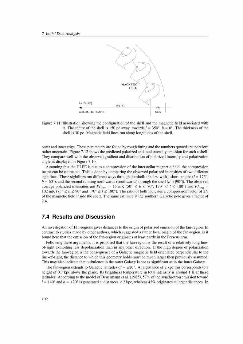
7 Initial Data Analysis
SUN
150 PC
GALACTIC PLANE
l = 350 deg
MAGNETIC FIELD
Figure 7.11: Illustration showing the configuration of the shell and the magnetic field associated withit. The centre of the shell is 150 pc away, towards l = 350◦, b = 0◦. The thickness of theshell is 30 pc. Magnetic field lines run along longitudes of the shell.
outer and inner edge. These parameters are found by rough fitting and the numbers quoted are thereforerather uncertain. Figure 7.12 shows the predicted polarized and total intensity emission for such a shell.They compare well with the observed gradient and distribution of polarized intensity and polarizationangle as displayed in Figure 7.10.
Assuming that the HLPE is due to a compression of the interstellar magnetic field, the compressionfactor can be estimated. This is done by comparing the observed polarized intensities of two differentsightlines. These sightlines run different ways through the shell: the first with a short lengths (l = 175◦,b = 60◦), and the second running northwards (southwards) through the shell (b ≈ |90◦|). The observedaverage polarized intensities are PIshort = 15 mK (50◦ ≤ b ≤ 70◦, 170◦ ≤ l ≤ 180◦) and PIlong =
102 mK (75◦ ≤ b ≤ 90◦ and 170◦ ≤ l ≤ 180◦). The ratio of both indicates a compression factor of 2.9of the magnetic field inside the shell. The same estimate at the southern Galactic pole gives a factor of2.4.
7.4 Results and Discussion
An investigation of H -regions gives distances to the origin of polarized emission of the fan-region. Incontrast to studies made by other authors, which suggested a rather local origin of the fan-region, is itfound here that the emission of the fan-region originates at least partly in the Perseus arm.
Following these arguments, it is proposed that the fan-region is the result of a relatively long line-of-sight exhibiting less depolarization than in any other direction. If the high degree of polarizationtowards the fan-region is the consequence of a Galactic magnetic field orientated perpendicular to theline-of-sight, the distance to which this geometry holds must be much larger then previously assumed.This may also indicate that turbulence in the outer Galaxy is not as significant as in the inner Galaxy.
The fan-region extends to Galactic latitudes of ∼ ±20◦. At a distance of 2 kpc this corresponds to aheight of 0.7 kpc above the plane. Its brightness temperature in total intensity is around 1 K at theselatitudes. According to the model of Beuermann et al. (1985), 57% of the synchrotron emission towardl = 140◦ and b = ±20◦ is generated at distances < 2 kpc, whereas 43% originates at larger distances. In
102
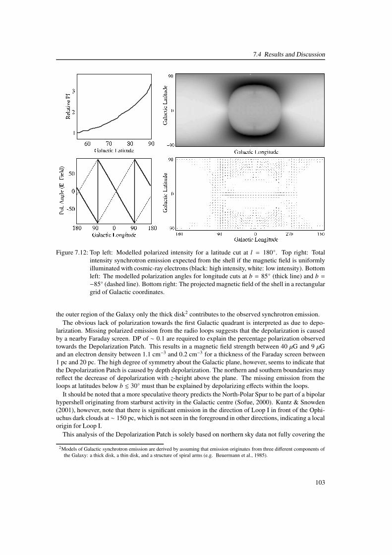
7.4 Results and Discussion
Figure 7.12: Top left: Modelled polarized intensity for a latitude cut at l = 180◦. Top right: Totalintensity synchrotron emission expected from the shell if the magnetic field is uniformlyilluminated with cosmic-ray electrons (black: high intensity, white: low intensity). Bottomleft: The modelled polarization angles for longitude cuts at b = 85◦ (thick line) and b =−85◦ (dashed line). Bottom right: The projected magnetic field of the shell in a rectangulargrid of Galactic coordinates.
the outer region of the Galaxy only the thick disk2 contributes to the observed synchrotron emission.The obvious lack of polarization towards the first Galactic quadrant is interpreted as due to depo-
larization. Missing polarized emission from the radio loops suggests that the depolarization is causedby a nearby Faraday screen. DP of ∼ 0.1 are required to explain the percentage polarization observedtowards the Depolarization Patch. This results in a magnetic field strength between 40 µG and 9 µGand an electron density between 1.1 cm−3 and 0.2 cm−3 for a thickness of the Faraday screen between1 pc and 20 pc. The high degree of symmetry about the Galactic plane, however, seems to indicate thatthe Depolarization Patch is caused by depth depolarization. The northern and southern boundaries mayreflect the decrease of depolarization with z-height above the plane. The missing emission from theloops at latitudes below b . 30◦ must than be explained by depolarizing effects within the loops.
It should be noted that a more speculative theory predicts the North-Polar Spur to be part of a bipolarhypershell originating from starburst activity in the Galactic centre (Sofue, 2000). Kuntz & Snowden(2001), however, note that there is significant emission in the direction of Loop I in front of the Ophi-uchus dark clouds at ∼ 150 pc, which is not seen in the foreground in other directions, indicating a localorigin for Loop I.
This analysis of the Depolarization Patch is solely based on northern sky data not fully covering the
2Models of Galactic synchrotron emission are derived by assuming that emission originates from three different components ofthe Galaxy: a thick disk, a thin disk, and a structure of spiral arms (e.g. Beuermann et al., 1985).
103

7 Initial Data Analysis
fourth Galactic quadrant. An all-sky polarization map3 will soon become available. This will allowthe investigation of the properties of the Depolarization Patch more accurately and help understand itsorigin.
The polarized emission observed at high Galactic latitudes, the HLPE, can be modelled by assumingthat the Sun is located within a magnetized shell. In this model the intensity and polarization angleof the observed synchrotron emission are given by the strength and direction of the magnetic fieldcomponent perpendicular to the line-of-sight. A compression factor of the field inside the shell of∼ 3 relative to an ambient magnetic field can be derived. The centre and spatial extent of this shellcorrespond well to that of Loop I.
The agreement in centre and size of the HLPE with Loop I suggest a common origin. It is thereforeproposed that the HLPE is a magnetic shell associated with Loop I: either a magnetic field aroundthe H bubble or the compressed field around an evolved SNR. This is supported by the previouslymentioned association of H and dust filaments with the HLPE.
These investigations can only provide the basis for deeper analysis. Improvement in sky coverageis required to strengthen arguments for the distance of the fan-region, given by the depolarization ofH -regions. A multi-wavelength analysis of the Depolarization Patch must follow, taking X-ray anddust emission into account. Finally, better sampled data may show correlations between the HLPE andfilaments in dust and H more clearly.
3achieved by combining the 26-m Survey and the Villa-Elisa Survey (Testori et al., 2004)
104
8 Summary and Conclusion
My research objective was to realize a polarization survey covering the northern sky, which wouldallow the absolute calibration of recent high-resolution polarization observations. During an observingtime of 7 months, I was able to perform 168 fully calibrated drift scans, utilizing the 26-m Telescopeof the DRAO. The resulting sky coverage and sensitivity exceeds that of the so far available data of thenorthern sky, observed in the 1960’s and 70’s with the Dwingeloo telescope. By comparing drift scanswith data obtained with the Effelsberg 100-m telescope an accurate brightness temperature scale of thenew survey could be established.
In areas where the sampling of the LDS is too sparse, the new 26-m Survey makes proper calibra-tion of high-resolution data possible. I showed that a correct representation of large-scale emission inStokes U and Q down to the lowest spatial frequencies is mandatory for the analysis of diffuse polarizedemission, and that the 26-m Survey provides these data to correct for missing emission components inhigh-resolution data.
Aside from making absolutely calibrated data available for calibration purposes, the 26-m Survey isa valuable astronomical product in its own right, revealing unknown features and providing valuableinformation on the Galactic polarized foreground. By an initial analysis of the new data I was able toreach the following conclusions: 1) Depolarizing H -regions towards the highly polarized fan-regionreveal a larger distance to the origin of polarized emission than previously believed. As a consequenceturbulence of the magneto-ionic medium in the outer Galaxy towards the fan-region must be smallto allow the relatively long line-of-sight in polarization; 2) An apparent lack of polarized emissiontowards the first Galactic quadrant is noted and is interpreted as due to depolarization. Based on thenon-observation of polarized emission from the radio loops, the possibility of a local Faraday screencausing depolarization is discussed. Other arguments taking into account effects within the loops areconsidered; 3) Polarized emission at high Galactic latitudes is found and modelled assuming that theSun is located within a magnetic shell that emits synchrotron emission.
8.1 Major Contributions
In summary, my research involved the further development of the receiving system of the DRAO 26-mtelescope to make measurements of linear polarization possible. Moreover, applicable data processingroutines needed to be developed to properly calibrate the raw data. This required the solution of prob-lems such as the system temperature variations recognized during data reduction, and the developmentof a suitable interpolation routine. The major contributions of my exploration of the Galactic polarizedemission are as follows:
• Realization and calibration of the Low-Resolution DRAO Survey of Polarized Emission at1.4 GHz.
• Demonstration of the necessity of absolute calibrating diffuse polarized emission and the capa-bility of the 26-m Survey in providing the spatial frequencies required for this calibration.
• Evidence that a significant amount of polarized emission from the fan-region originates in or be-yond the Perseus spiral arm. Hence, the intense polarized emission is received from much larger
105

8 Summary and Conclusion
distances than in any other direction. This can be used to derive constraints on the properties ofthe magneto-ionic medium of the outer Galaxy.
• First description of a lack of polarized emission revealed by low percentage polarization towardsthe first Galactic quadrant.
• First observational evidence for polarized radio emission at 1.4 GHz at high Galactic latitudes.
8.2 Future Work
Observations for the 26-m Survey I have presented here are continuing. Currently (by March 2005),the coverage of the northern sky with drift scans has reached 43%. These data must be incorporatedand will result in a considerable improvement of the 26-m Survey in terms of resolution, sensitivity,and error. It is planned to make the extended data public.
The incorporation of the latest data of the 26-m Survey will allow to substantiate arguments for therevised distance to the fan-region as described in this thesis. A larger number of well justified H -regions acting as depolarizing Faraday screens will provide data for the study of the local synchrotronemissivity.
The inclusion of data from the southern sky polarization survey (Testori et al., 2004) is required toconfine boundaries of the Depolarization Patch more accurately. An improvement in sampling couldalso allow to investigate small-scale fluctuations towards the first quadrant, which could reveal its ori-gin.
Another point concerns the observing scheme. Here, it is desirable to apply an independent calibra-tion instead of relying on the LDS. This becomes even more important in view of the planned upgradeof the 26-m telescope to allow the simultaneous measurement of polarization at multiple frequencies.Also, an improved model for ground radiation should be developed, possibly taking time-variabilityinto account.
106
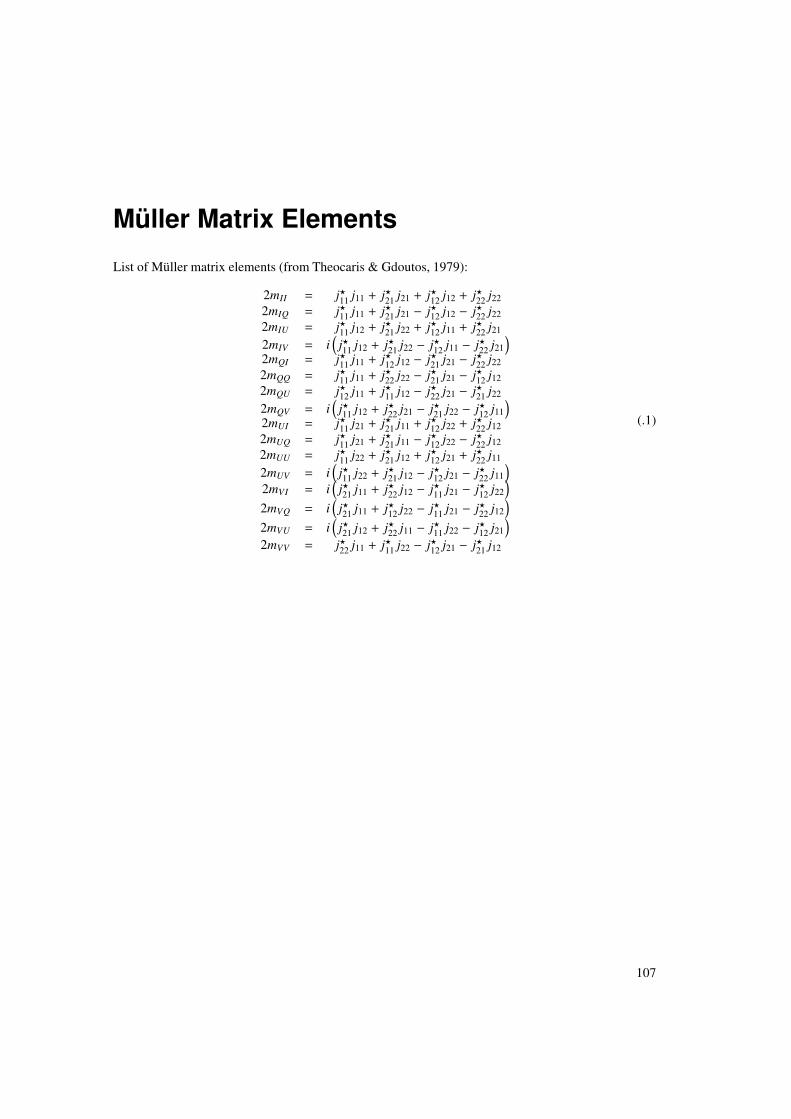
Müller Matrix Elements
List of Müller matrix elements (from Theocaris & Gdoutos, 1979):
2mII = j?11 j11 + j?21 j21 + j?12 j12 + j?22 j22
2mIQ = j?11 j11 + j?21 j21 − j?12 j12 − j?22 j222mIU = j?11 j12 + j?21 j22 + j?12 j11 + j?22 j21
2mIV = i(
j?11 j12 + j?21 j22 − j?12 j11 − j?22 j21
)
2mQI = j?11 j11 + j?12 j12 − j?21 j21 − j?22 j22
2mQQ = j?11 j11 + j?22 j22 − j?21 j21 − j?12 j122mQU = j?12 j11 + j?11 j12 − j?22 j21 − j?21 j22
2mQV = i(
j?11 j12 + j?22 j21 − j?21 j22 − j?12 j11
)
2mUI = j?11 j21 + j?21 j11 + j?12 j22 + j?22 j12
2mUQ = j?11 j21 + j?21 j11 − j?12 j22 − j?22 j122mUU = j?11 j22 + j?21 j12 + j?12 j21 + j?22 j11
2mUV = i(
j?11 j22 + j?21 j12 − j?12 j21 − j?22 j11
)
2mVI = i(
j?21 j11 + j?22 j12 − j?11 j21 − j?12 j22
)
2mVQ = i(
j?21 j11 + j?12 j22 − j?11 j21 − j?22 j12
)
2mVU = i(
j?21 j12 + j?22 j11 − j?11 j22 − j?12 j21
)
2mVV = j?22 j11 + j?11 j22 − j?12 j21 − j?21 j12
(.1)
107

Müller Matrix Elements
108

Bibliography
Altenhoff, W., Mezger, P. G., Strassl, H., Wendker, H., & Westerhout, G. 1960, Veröffentlichunnge derUniversitäts-Sternwarte zu Bonn, 59
Beck, R. 2001, Space Science Reviews, 99, 243
Berkhuijsen, E. M. 1971, Astronomy and Astrophysics, 14, 359
—. 1975, Astronomy and Astrophysics, 40, 311
Berkhuijsen, E. M. & Brouw, W. N. 1963, Bull. Astron. Inst. Netherlands, 17, 185
Berkhuijsen, E. M., Brouw, W. N., Muller, C. A., & Tinbergen, J. 1964, Bull. Astron. Inst. Netherlands,17, 465
Berkhuijsen, E. M., Haslam, C. G. T., & Salter, C. J. 1971, Astronomy and Astrophysics, 14, 252
Bernardi, G., Carretti, E., Fabbri, R., Sbarra, C., Poppi, S., & Cortiglioni, S. 2004, in The MagnetizedInterstellar Medium, 207–212
Bertiau, F. C. 1958, Astrophysical Journal, 128, 533
Beuermann, K., Kanbach, G., & Berkhuijsen, E. M. 1985, Astronomy and Astrophysics, 153, 17
Bingham, R. G. 1966, Monthly Notices of the RAS, 134, 327
Bingham, R. G. & Shakeshaft, J. R. 1967, Monthly Notices of the RAS, 136, 347
Bochkarev, N. G. 1987, Astrophysics and Space Science, 138, 229
Born, M. & Wolf, E. 1965, Principles of optics. Electromagnetic theory of propagation, interferenceand diffraction of light (Oxford: Pergamon Press, |c1965, 3rd (revised) ed.)
Brouw, W. N., Muller, C. A., & Tinbergen, J. 1962, Bull. Astron. Inst. Netherlands, 16, 213
Brouw, W. N. & Spoelstra, T. A. T. 1976, Astronomy and Astrophysics, Supplement, 26, 129
Burn, B. J. 1966, Monthly Notices of the RAS, 133, 67
Campbell, R. M. 1999, New Astronomy Review, 43, 617
Conway, R. G. & Kronberg, P. P. 1969, Monthly Notices of the RAS, 142, 11
Cox, D. P. & Reynolds, R. J. 1987, Annual Review of Astron and Astrophys, 25, 303
Cruz-Gonzalez, C., Recillas-Cruz, E., Costero, R., Peimbert, M., & Torres-Peimbeert, S. 1974, RevistaMexicana de Astronomia y Astrofisica, 1, 211
de Geus, E. J. & Burton, W. B. 1991, Astronomy and Astrophysics, 246, 559
Dickey, J. M. 1997, Astrophysical Journal, 488, 258
Dickey, J. M., McClure-Griffiths, N., Gaensler, B., Green, A., Haynes, R., & Wieringa, M. 1999, inAstronomical Society of the Pacific Conference Series, 27–+
Dieter, N. H. 1964, Astronomical Journal, 69, 137
109

Bibliography
Duncan, A. R., Haynes, R. F., Jones, K. L., & Stewart, R. T. 1997, Monthly Notices of the RAS, 291,279
Duncan, A. R., Haynes, R. F., Reich, W., Reich, P., & Gray, A. D. 1998, Monthly Notices of the RAS,299, 942
Egger, R. J. & Aschenbach, B. 1995, Astronomy and Astrophysics, 294, L25
Egger, R. J., Freyberg, M. J., & Morfill, G. E. 1996, Space Science Reviews, 75, 511
Erickson, W. C., Perley, R. A., Flatters, C., & Kassim, N. E. 2001, Astronomy and Astrophysics, 366,1071
Ferlet, R. 1999, Astronomy and Astrophysics Reviews, 9, 153
Fich, M. & Blitz, L. 1984, Astrophysical Journal, 279, 125
Fich, M., Blitz, L., & Stark, A. A. 1989, Astrophysical Journal, 342, 272
Finkbeiner, D. P. 2003, Astrophysical Journal, Supplement, 146, 407
Freyberg, M. J. & Breitschwerdt, D. 2001, in Astronomische Gesellschaft Meeting Abstracts, 104–+
Gaensler, B. M., Dickey, J. M., McClure-Griffiths, N. M., Green, A. J., Wieringa, M. H., & Haynes,R. F. 2001, Astrophysical Journal, 549, 959
Gray, A. D., Landecker, T. L., Dewdney, P. E., & Taylor, A. R. 1998, Nature, 393, 660
Gray, A. D., Landecker, T. L., Dewdney, P. E., Taylor, A. R., Willis, A. G., & Normandeau, M. 1999,Astrophysical Journal, 514, 221
Haslam, C. G. T., Large, M. I., & Quigley, M. J. S. 1964, Monthly Notices of the RAS, 127, 273
Haslam, C. G. T., Stoffel, H., Salter, C. J., & Wilson, W. E. 1982, Astronomy and Astrophysics, Sup-plement, 47, 1
Haverkorn, M., Gaensler, B. M., McClure-Griffiths, N. M., Dickey, J. M., & Green, A. J. 2004a,Astrophysical Journal, 609, 776
Haverkorn, M., Katgert, P., & de Bruyn, A. G. 2004b, Astronomy and Astrophysics, 427, 549
Heiles, C. 1967, Astrophysical Journal, Supplement, 15, 97
Heiles, C. 2002, in Astronomical Society of the Pacific Conference Series, 131–152
Heiles, C., Perillat, P., Nolan, M., Lorimer, D., Bhat, R., Ghosh, T., Howell, E., Lewis, M., O’Neil, K.,Salter, C., & Stanimirovic, S. 2001, PASP, 113, 1247
Higgs, L. A. 1967, Bulletin of the Astronomical Institute of the Netherlands Supplement Series, 2, 59
Higgs, L. A. & Tapping, K. F. 2000, Astronomical Journal, 120, 2471
Howell, T. F. & Shakeshaft, J. R. 1966, Nature, 210, 1318
Jansky, K. G. 1933, Proc. I.R.E., 21, 1387
Jones, R. C. 1941, Journal of the Optical Society of America (1917-1983), 31, 488
Junkes, N. 1986, Mitteilungen der Astronomischen Gesellschaft Hamburg, 65, 224
Kafatos, M. C. & Morrison, P. 1973, Astronomy and Astrophysics, 26, 71
Kiepenheuer, K. O. 1950, Physical Review, 79, 738
Knee, L. B. G. 1997, DRAO Internal Report
Kothes, R., Landecker, T. L., & Wolleben, M. 2004a, Astrophysical Journal, 607, 855
Kothes, R., Landecker, T. L., Wolleben, M., Foster, T., & Reich, W. 2004b, DRAO News
110

Bibliography
Kraus, J. D. 1966, Radio astronomy (New York: McGraw-Hill, 1966)
Kuntz, K. D. & Snowden, S. L. 2001, Astrophysical Journal, 554, 684
Landecker, T. L., Uyaniker, B., & Kothes, R. 2002, in AIP Conf. Proc. 609: Astrophysical PolarizedBackgrounds, 9–12
Large, M. I., Quigley, M. F. S., & Haslam, C. G. T. 1966, Monthly Notices of the RAS, 131, 335
Large, M. I., Quigley, M. J. S., & Haslam, C. G. T. 1962, Monthly Notices of the RAS, 124, 405
Mathewson, D. S., Broten, N. W., & Cole, D. J. 1965, Australian Journal of Physics, 18, 665
—. 1966, Australian Journal of Physics, 19, 93
McMullin, J. P., Golap, K., & Myers, S. T. 2004, in Astronomical Society of the Pacific ConferenceSeries, 468–+
Milogradov-Turin, J. & Urosevic, D. 1997, Bulletin Astronomique de Belgrade, 155, 41
Mueller, H. 1948, J. Opt. Soc. Am., 38, 661
Muller, C. A., Berkhuijsen, E. M., Brouw, W. N., & Tinbergen, J. 1963, Nature, 200, 155
Pacholczyk, A. G. 1970, Radio astrophysics. Nonthermal processes in galactic and extragalactic sources(Series of Books in Astronomy and Astrophysics, San Francisco: Freeman, 1970)
Quigley, M. J. S. & Haslam, C. G. T. 1965, Nature, 208, 741
Razin, V. A., Khrulev, V. V., Fedorov, V. T., Volokhov, S. A., Melnikov, A. A., Paseka, A. M., &Pupysheva, L. V. 1968, Izvestiya VUZ. Radiofizika, 11, 1461
Reber, G. 1944, Astrophysical Journal, 100, 279
Reich, P. & Reich, W. 1986, Astronomy and Astrophysics, Supplement, 63, 205
Reich, W. 1982, Astronomy and Astrophysics, Supplement, 48, 219
Reich, W., Fürst, E., Reich, P., Uyaniker, B., Wielebinski, R., & Wolleben, R. 2004, in The MagnetizedInterstellar Medium, 45–50
Reich, W., Reich, P., & Fuerst, E. 1990, Astronomy and Astrophysics, Supplement, 83, 539
Reich, W. & Wielebinski, R. 2000, Radio Polarization: a New Probe of the Galaxy, Proceedings of aWorkshop held at Université de Mentréal
Rohlfs, K. & Wilson, T. L. 1996, Tools of Radio Astronomy (Tools of Radio Astronomy, XVI, 423pp. 127 figs., 20 tabs.. Springer-Verlag Berlin Heidelberg New York. Also Astronomy and Astro-physics Library)
Rubin, V. C., Burtley, J., Kiasatpoor, A., Klock, B., Pease, G., Rutscheidt, E., & Smith, C. 1962,Astronomical Journal, 67, 491
Salter, C. J. 1983, Bulletin of the Astronomical Society of India, 11, 1
Schott, G. A. 1907, Ann. Physik
Siringo, G., Kreysa, E., Reichertz, L. A., & Menten, K. M. 2004, Astronomy and Astrophysics, 422,751
Snowden, S. L., Freyberg, M. J., Plucinsky, P. P., Schmitt, J. H. M. M., Truemper, J., Voges, W., Edgar,R. J., McCammon, D., & Sanders, W. T. 1995, Astrophysical Journal, 454, 643
Sofue, Y. 2000, Astrophysical Journal, 540, 224
Spoelstra, T. A. T. 1971, Astronomy and Astrophysics, 13, 237
111

Bibliography
—. 1984, Astronomy and Astrophysics, 135, 238
Tauber, J. A. 2004, in The Magnetized Interstellar Medium, 191–199
Taylor, A. R., Gibson, S. J., Peracaula, M., Martin, P. G., Landecker, T. L., Brunt, C. M., Dewdney,P. E., Dougherty, S. M., Gray, A. D., Higgs, L. A., Kerton, C. R., Knee, L. B. G., Kothes, R., Purton,C. R., Uyaniker, B., Wallace, B. J., Willis, A. G., & Durand, D. 2003, Astronomical Journal, 125,3145
Testori, J. C., Reich, P., & Reich, W. 2004, in The Magnetized Interstellar Medium, 57–62
Theocaris, P. S. & Gdoutos, E. E., eds. 1979, Matrix theory of photoelasticity
Tinbergen, J. 1996, Astronomical polarimetry (Cambridge, New York: Cambridge University Press,|c1996, ISBN 0521475317)
Uyaniker, B., Fürst, E., Reich, W., Reich, P., & Wielebinski, R. 1999, Astronomy and Astrophysics,Supplement, 138, 31
Uyaniker, B., Fuerst, E., Reich, W., Reich, P., & Wielebinski, R. 1998, Astronomy and Astrophysics,Supplement, 132, 401
Verschuur, G. L. 1968, The Observatory, 88, 15
von Hoensbroech, A. & Xilouris, K. M. 1997, Astronomy and Astrophysics, Supplement, 126, 121
Weaver, H. 1979, in IAU Symp. 84: The Large-Scale Characteristics of the Galaxy, 295–298
Westerhout, G., Seeger, C. L., Brouw, W. N., & Tinbergen, J. 1962, Bull. Astron. Inst. Netherlands, 16,187
Westfold, K. C. 1959, Astrophysical Journal, 130, 241
Wielebinski, R. & Shakeshaft, F. R. 1964, Monthly Notices of the RAS, 128, 19
Wielebinski, R., Shakeshaft, J. R., & Pauliny-Toth, I. I. K. 1962, The Observatory, 82, 158
Wieringa, M. H., de Bruyn, A. G., Jansen, D., Brouw, W. N., & Katgert, P. 1993, Astronomy andAstrophysics, 268, 215
Wilkinson, A. & Smith, F. G. 1974, Monthly Notices of the RAS, 167, 593
Willingale, R., Hands, A. D. P., Warwick, R. S., Snowden, S. L., & Burrows, D. N. 2003, MonthlyNotices of the RAS, 343, 995
Wolleben, M. 2001, Diplomarbeit, Universität Bonn
Wolleben, M. & Reich, W. 2004, Astronomy and Astrophysics, 427, 537
112

List of Tables
3.1 Receiver and antenna specifications . . . . . . . . . . . . . . . . . . . . . . . . . . . 233.2 Interface card specifications. . . . . . . . . . . . . . . . . . . . . . . . . . . . . . . . 333.3 Survey specifications . . . . . . . . . . . . . . . . . . . . . . . . . . . . . . . . . . . 473.4 Summarized listing of survey drift scans. . . . . . . . . . . . . . . . . . . . . . . . . . 483.5 Observing dates of the elevation scans used for the determination of ground radiation
profiles. . . . . . . . . . . . . . . . . . . . . . . . . . . . . . . . . . . . . . . . . . . 48
4.1 Parameters used for the correction of system temperature fluctuations. . . . . . . . . . 584.2 Error budget of the 26-m Survey. . . . . . . . . . . . . . . . . . . . . . . . . . . . . . 66
7.1 List of H regions visible in polarization. . . . . . . . . . . . . . . . . . . . . . . . . 94
113

List of Tables
114

List of Figures
1.1 Polarization Map of the North Polar Spur . . . . . . . . . . . . . . . . . . . . . . . . 11.2 Leiden/Dwingeloo Polarization Survey at 1.4 GHz . . . . . . . . . . . . . . . . . . . 21.3 Polarized brightness temperatures of two frequently used calibration points . . . . . . 41.4 Effect of missing spatial information in polarized intensity maps . . . . . . . . . . . . 61.5 Effect of missing large-scale structures on polarized intensity and polarization angle . . 71.6 Two cases in RM-studies . . . . . . . . . . . . . . . . . . . . . . . . . . . . . . . . . 81.7 Vectors in the two cases of RM-studies . . . . . . . . . . . . . . . . . . . . . . . . . . 9
3.1 Picture of the 26-m telescope of the DRAO . . . . . . . . . . . . . . . . . . . . . . . 203.2 Picture of the 1.4 GHz receiver of the DRAO 26-m . . . . . . . . . . . . . . . . . . . 213.3 Block diagram of the 1410 MHz continuum receiver . . . . . . . . . . . . . . . . . . 223.4 Phase tracking of the two polarization components . . . . . . . . . . . . . . . . . . . 243.5 Functional block diagram of a quadrature hybrid . . . . . . . . . . . . . . . . . . . . . 253.6 Calculated response of the system taking phase errors and power level mismatches in
the pre-hybrid part into account . . . . . . . . . . . . . . . . . . . . . . . . . . . . . . 313.7 Calculation of the sensitivity loss for a linear phase gradient across the observing band 333.8 Flow diagram of the data stream . . . . . . . . . . . . . . . . . . . . . . . . . . . . . 343.9 Screenshot of the data distribution program (Mom) . . . . . . . . . . . . . . . . . . . 363.10 Screenshot of the Waterfall Display . . . . . . . . . . . . . . . . . . . . . . . . . . . 373.11 Screenshot of the raw data reduction program (DRP) . . . . . . . . . . . . . . . . . . 383.12 Response pattern of the DRAO 26-m telescope . . . . . . . . . . . . . . . . . . . . . 423.13 Example map of the TEC . . . . . . . . . . . . . . . . . . . . . . . . . . . . . . . . . 443.14 Ground radiation is received through the side and back lobes of the antenna . . . . . . 46
4.1 Reduction chain . . . . . . . . . . . . . . . . . . . . . . . . . . . . . . . . . . . . . . 504.2 Example for RFI in one of the total power channels . . . . . . . . . . . . . . . . . . . 514.3 Ground radiation profiles determined on the basis of elevation scans . . . . . . . . . . 564.4 Example of system temperature drifts . . . . . . . . . . . . . . . . . . . . . . . . . . 574.5 Uncleaned map of polarized intensity . . . . . . . . . . . . . . . . . . . . . . . . . . 584.6 Two example scans through the Taurus complex and Cassiopeia-A . . . . . . . . . . . 614.7 8 hour night-time observation of the northern celestial pole . . . . . . . . . . . . . . . 624.8 Correlation coefficients of Stokes U and Q and number of matches plotted versus the
congruence radius . . . . . . . . . . . . . . . . . . . . . . . . . . . . . . . . . . . . . 634.9 Correlation of Stokes U and Q intensities from the DRAO 26-m Survey with the
Dwingeloo survey . . . . . . . . . . . . . . . . . . . . . . . . . . . . . . . . . . . . . 644.10 Stokes U and Q of repeated scans . . . . . . . . . . . . . . . . . . . . . . . . . . . . 65
6.1 Stokes U difference map . . . . . . . . . . . . . . . . . . . . . . . . . . . . . . . . . 826.2 Stokes Q difference map . . . . . . . . . . . . . . . . . . . . . . . . . . . . . . . . . 83
115

List of Figures
6.3 Polarized intensity difference map . . . . . . . . . . . . . . . . . . . . . . . . . . . . 84
7.1 Sketch of prominent features in the polarized intensity map . . . . . . . . . . . . . . . 867.2 Structure of the LISM . . . . . . . . . . . . . . . . . . . . . . . . . . . . . . . . . . . 907.3 Sketch highlighting the filaments of the North-Polar Spur . . . . . . . . . . . . . . . . 927.4 Depolarization at the southern edge of the emission feature G343+34 . . . . . . . . . 937.5 Drift scans through H regions located toward the fan region . . . . . . . . . . . . . . 957.6 Polarized intensity towards the California nebula . . . . . . . . . . . . . . . . . . . . 967.7 Polarized intensity towards Sh2-229, Sh2-236, and Orion complex . . . . . . . . . . . 977.8 O-stars whose Strömgren spheres possibly depolarize background emission . . . . . . 987.9 408 MHz and soft X-ray emission of the North-Polar Spur . . . . . . . . . . . . . . . 997.10 Observed increase of polarized intensity toward the northern and southern Galactic poles 1017.11 Illustration showing the configuration of the shell and the magnetic field associated with it1027.12 Modelled polarized intensity and angle . . . . . . . . . . . . . . . . . . . . . . . . . . 103
116